Character Aware Decoder for Translation into Morphologically Rich Languages

Character-Aware Decoder for Translation

into Morphologically Rich Languages

Adithya Renduchintala∗ _{and Pamela Shapiro}∗ _{and Kevin Duh and Philipp Koehn} Department of Computer Science

Johns Hopkins University

{adi.r,pshapiro,phi_}@jhu.edu [email protected]

Abstract

Neural machine translation (NMT) sys-tems operate primarily on words (or sub-words), ignoring lower-level patterns of morphology. We present a character-aware decoder designed to capture such patterns when translating into morpho-logically rich languages. We achieve character-awareness by augmenting both the softmax and embedding layers of an attention-based encoder-decoder model with convolutional neural networks that operate on the spelling of a word. To in-vestigate performance on a wide variety of morphological phenomena, we translate English into 14 typologically diverse tar-get languages using the TED multi-tartar-get dataset. In this low-resource setting, the character-aware decoder provides consis-tent improvements with BLEU score gains of up to +3.05. In addition, we analyze the relationship between the gains obtained and properties of the target language and find evidence that our model does indeed exploit morphological patterns.

1 Introduction

Traditional attention-based encoder-decoder neu-ral machine translation (NMT) models learn word-level embeddings, with a continuous representa-tion for each unique word type (Bahdanau et al., 2015). However, this results in a long tail of rare words for which we do not learn good representa-tions. More recently, it has become standard

prac-c

2019 The authors. This article is licensed under a Creative Commons 4.0 licence, no derivative works, attribution, CC-BY-ND.

∗_{Equal Contribution}

tice to mitigate the vocabulary size problem with Byte-Pair Encoding (BPE) (Gage, 1994; Sennrich et al., 2016). BPE iteratively merges consecutive characters into larger chunks based on their fre-quency, which results in the breaking up of less common words into “subword units.”

While BPE addresses the vocabulary size prob-lem, the spellings of the subword units are still ig-nored. On the other hand, purelycharacter-level NMT translates one character at a time and can im-plicitly learn about morphological patterns within words as well as generalize to unseen vocabulary. Recently, Cherry et al. (2018) show that very deep character-level models can outperform BPE, how-ever, the smallest data size evaluated was 2 million sentences, so it is unclear if the results hold for low-resource settings and when translating into a range of different morphologically rich languages. Furthermore, tuning deep character-level models is expensive, even for low-resource settings.1

A middle-ground alternative is character-aware word-level modeling. Here, the NMT system op-erates over words but uses word embeddings that are sensitive to spellings and thereby has the abil-ity to learn morphological patterns in the language. Such character-aware approaches have been ap-plied successfully in NMT to the source-side word embedding layer (Costa-juss`a and Fonollosa, 2016), but surprisingly, similar gains have not been achieved on the target side (Belinkov et al., 2017). While source-side character-aware models only need to make the source embedding layer character-aware, on the target-side we require both thetarget embedding layerand thesoftmax layer2

1_{The dropout rate was found to be critical in Cherry et al.}

(2018), and each tuning run takes much longer due to longer sequence lengths.

to be character-aware, which presents additional challenges. We find that the trivial application of methods from Costa-juss`a and Fonollosa (2016) to these target-side embeddings results in significant drop in performance. Instead, we propose mixing compositional and standard word embeddings via a gating function. While simple, we find it is criti-cal to successful target-side character awareness.

It is worth noting that unlike some purely character-level methods our aim is not to gener-ate novel words, though this method can function on top of subword methods which do so (Shapiro and Duh, 2018). Rather, the character-aware rep-resentations decrease the sparsity of embeddings for rare words or subwords, which are a problem in low-resource morphologically rich settings. We summarize our contribution as follows:

1. We propose a method for utilizing character-aware embeddings in an NMT decoder that can be used over word or subword sequences.

2. We explore how our method interacts with BPE over a range of merge operations (in-cluding word-level and purely character-level) and highlight that there is no “typical BPE” setting for low-resource NMT.

3. We evaluate our model on14target languages and observe consistent improvements over baselines. Furthermore, we analyze to what extent the success of our method corresponds to improved handling of target language mor-phology.

2 Related Work

NMT has benefited from character-aware word representations on the source side (Costa-juss`a and Fonollosa, 2016), which follows language model-ing work by Kim et al. (2016) and generate source-side input embeddings using a CNN over the char-acter sequence of each word. Further analysis re-vealed that hidden states of such character-aware models have increased knowledge of morphology (Belinkov et al., 2017). They additionally try using character-aware representations in the target side embedding layer, leaving the softmax matrix with standard word representations, and found no im-provements.

Our work is also aligned with the character-aware models proposed in (Kim et al., 2016), but

projection.

we additionally employ a gating mechanism be-tween character-aware representations and stan-dard word representations similar to language modeling work by (Miyamoto and Cho, 2016). However, our gating is a learned type-specific vec-tor rather than a fixed hyperparameter.

There is additionally a line of work on purely character-level NMT, which generates words one character at a time (Ling et al., 2015; Chung et al., 2016; Passban et al., 2018). While initial sults here were not strong, Cherry et al. (2018) re-visit this with deeper architectures and sweeping dropout parameters and find that they outperform BPE across settings of the merge hyperparame-ter. They examine different data sizes and observe improvements in the smaller data size settings— however, the smallest size is about 2 million sen-tence pairs. In contrast, we look at a smaller order of magnitude data size and present an alternate ap-proach which doesn’t require substantial tuning of parameters across different languages.

Finally, Byte-Pair Encoding (BPE) (Sennrich et al., 2016) has become a standard preprocessing step in NMT pipelines and provides an easy way to generate sequences with a mixture of full words and word fragments. Note that BPE splits are ag-nostic to any morphological pattern present in the language, for example the tokenpolitelyin our dataset is split into pol+itely, instead of the linguistically plausible split polite+ly.3 _Our

approach can be applied to word-level sequences and sequences at any BPE merge hyperparameter greater than0. Increasing the hyperparameter re-sults in more words and longer subwords that can exhibit morphological patterns. Our goal is to ex-ploit these morphological patterns and enrich the word (or subword) representations with character-awareness.

3 Encoder-Decoder NMT

An attention-based encoder-decoder network (Bahdanau et al., 2015; Luong et al., 2015) models the probability of a target sentenceyof length J given a source sentencexas:

p(y_|x) =

J

Y

j=1

p(yj |y0:j−1,x;θ) (1)

where θ represents all the parameters of the

generated by:

p(yj |y0:j−1,x) =softmax(Wosj) (2)

where sj ∈ RD×1 is the decoder hidden state at

time j and Wo ∈ R|V|×D is the weight matrix of the softmax layer, which provides a continuous representation for target words.sj is computed

us-ing the followus-ing recurrence:

sj =tanh(Wc[cj;˜sj]) (3) ˜sj =f([sj−1;wsyj−1;˜sj−1]) (4)

where f is an LSTM cell.4 Ws ∈ R|V|×E is the target-side embedding matrix, which provides continuous representations for the previous tar-get word when used as input to the RNN. Here,

wsyj−1 ∈ R1×E is a row vector from the em-bedding matrixWs corresponding to the value of yj−1.Vis the target vocabulary set,Dis the is the

RNN size andE is embedding size. Often these matricesWoandWsare tied.

The context vector cj is obtained by taking a

weighted average over the concatenation of a bidi-rectional RNN encoder’s hidden states.

cj = I

X

i=1

αi,hi (5)

αi =

exp (˜s>_j Wahi)

P

lexp (˜s>jWahl)

(6)

The attention matrix Wa ∈ RD×H is learned jointly with the model, multiplying with the pre-vious decoder state and bidirectional encoder state

hi ∈ RH×1, normalized over encoder hidden

states via the softmax operation.

4 Character-Aware Extension

In this section we detail the incorporation of character-awareness into the two decoder embed-ding matrices Wo and Ws. To begin, we con-sider an example target side word (or subword in the case of preprocessing with BPE),cat. In both

Wo andWs, there exist row vectors, wocatand wscatthat contain the continuous vector represen-tation for the word cat. In a traditional NMT system, these vectors are learned as the entire net-work tries to maximize the objective in Equation 1. The objective does not require the vectors wocat 4_{Note that our notation diverges from Luong et al. (2015) so}

thatsjrefers to the state used to make the final predictions.

wv_std

v=cat

(a)

c a t

highw

ay

1

highw

ay

2

h/si hsi

wv

comp

v=cat

(b)

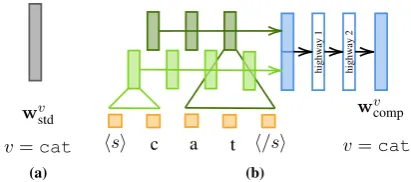
Figure 1:Different approaches to generating embeddings. (a)

standard word embedding that treats words as a single sym-bol. (b) CNN-based composition function. We use multiple CNNs with different kernel sizes over the character embed-dings. The resulting hidden states are combined into a single word embedding via max pooling. Note that (b) shows only2 convolution filters for clarity, in practice we use 4.

and wscat to model any aspect of the spelling of the word. Figure 1a illustrates a simple non-compositional word embedding.

At a high level, we can view our notion of character-awareness as a composition function comp(.;ω), parameterized by ω, that takes the

character sequence that makes up a word (i.e. its spelling) as input and then produces a continuous vector representation:

wcat_comp=comp(hsi,c,a,t,h/si;ω) (7)

ωis learned jointly with the overall objective.

Spe-cial characters hs_iand _h/s_i denote the beginning and end of sequence respectively.

Figure 1b illustrates our compositional approach to generating embeddings (Kim et al., 2016). First, a character-embedding layer converts the spelling of a word into a sequence of character embeddings. Next, we apply4convolution operations, with ker-nel sizes3,4,5and6, over the character sequence and the resulting output matrix is max-pooled. We set the output channel size of each convolution to

1

4 of the final desired embedding size. The

max-pooled vector from each convolution is concate-nated to create the composed word representation. Finally, we add highway layers to obtain the final embeddings.

4.1 Composed & Standard Gating

ing in thing is not compositional in the way that it is inrunning. Thus, we mix the compo-sitional and standard embedding vectors. We ex-pect standard embeddings to better represent the meaning of certain words, such has function words and other high-frequency words. For each word v in the vocabulary we also learn a gating vector gv _∈[0,1]1×D_.

gv =σ(wv_gate) (8)

Where,σ is a sigmoid operation and type-specific parameterswv

gateare jointly learned along with all

the other parameters of the composition function. These parameters are regularized to remain close to0using dropout. 5 _{Our final mixed word}

repre-sentation for each wordv∈ V is given by:

wv_mix=gvwv_std+ (1.−gv)wv_comp (9)

Wherewv

mixis the final word embedding, wvstd is

the standard word embedding, wv_comp is the

em-bedding by the composition function andgvis the

type-specific gating vector for thev’th word. The weight matrix is obtained by stacking the word vectors for each wordv _{∈ V}. The same represen-tation is used for the target embedding layer and the softmax layer i.e. we set wocat = wscat = wcat_mix, when v = cat. Thus, tying the compo-sition function parameters for the softmax weight matrix and the target-side embedding matrix.

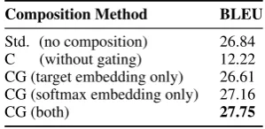
Experiments comparing the standard embed-ding model and the compositional embedembed-ding model with and without gating are summarized in Table 1. Row “C” shows the performance of naively using the composition function (which works in the source-side) on the target-side. We observe a catastrophic drop in BLEU (−14.62) compared to a standard NMT encoder-decoder. The Character-aware gated model(CG), however, outperforms the baseline by 0.91 BLEU points suggesting that the CNN composition function and standard embeddings work in a complementary fashion.

4.2 Large Vocabulary Approximation

In Equation 2 of the general NMT framework, the softmax operation generates a distribution over the output vocabulary. Our character-aware model re-quires a much larger computation graph as we ap-ply convolutions (and highway layers) over the 5_{However, in practice we found that this regularization did not}

affect performance noticeably in this setting.

Composition Method BLEU

Std. (no composition) 26.84 C (without gating) 12.22 CG (target embedding only) 26.61 CG (softmax embedding only) 27.16

CG (both) 27.75

Table 1:Experiments to determine the effectiveness of

com-position based embeddings and gated embeddings. We used en-de language pair from the TED multi-target dataset. Std. is our baseline with standard word embeddings, model C is the composition only model and CG combines the character-aware (composed) embedding and standard embedding via a gating function.

spellings (character embeddings) of entire target vocabulary, placing a limitation on the target vo-cabulary size for our model. Which is problematic for word-level modeling (without BPE).

To make our character-aware model accommo-date large target vocabulary sizes, we incorporate an approximation mechanism based on (Jean et al., 2015). Instead of computing the softmax over the entire vocabulary, we uniformly sample 20k vo-cabulary types and the vovo-cabulary types that are present in the training batch.

During decoding, we compute the forward pass

Wosj in Equation 2 in several splits of the

tar-get vocabulary. As no backward pass is required we clear the memory (i.e. delete the computation graph) after each split is computed.

5 Experiments

We evaluate our character aware model on14 dif-ferent languages in a low-resource setting. Ad-ditionally, we sweep over several BPE merge hy-perparameter settings from character-level to fully word-level for both our model and the baseline and find consistent gains in the character-aware model over the baseline. These gains are stable across all BPE merge hyperparameters all the way up to word-level where they are the highest.

5.1 Datasets

Language BPE Sweep @30k BPE @ Word-level

Std(Best BPE) CG(Best BPE) ∆ Std CG ∆ Std CG ∆

cs 20.57 (7.5k) 21.41 (7.5k) +0.84 18.73 21.28 +2.55 18.44 21.49 +3.05 uk 15.79 (7.5k) 16.60 (30k) +0.81 14.27 16.60 +2.33 12.94 15.30 +2.36 pl 16.76 (15k) 18.00 (30k) +1.24 15.98 18.00 +2.02 15.49 17.20 +1.71 tr 15.11 (7.5k) 15.83 (30k) +0.72 13.82 15.83 +2.01 12.58 14.75 +2.17 hu 16.61 (3.2k) 17.23 (15k) +0.62 15.45 17.21 +1.76 14.18 16.52 +2.34 he 23.36 (3.2k) 23.86 (30k) +0.50 22.47 23.86 +1.39 21.26 23.01 +1.75 pt 37.85 (15k) 38.35 (30k) +0.50 37.05 38.35 +1.30 37.13 38.36 +1.23 ar 16.22 (7.5k) 16.28 (30k) +0.06 15.05 16.28 +1.23 14.45 16.05 +1.60 de 27.37 (7.5k) 28.12 (30k) +0.75 26.94 28.12 +1.21 26.84 27.75 +0.91 ro 24.02 (3.2k) 24.20 (15k) +0.18 22.88 24.00 +1.12 22.39 23.27 +0.88 bg 31.63 (7.5k) 32.20 (15k) +0.57 30.92 31.90 +0.98 30.18 31.43 +1.25 fr 35.97 (1.6k) 36.17 (7.5k) +0.20 35.31 35.92 +0.61 35.28 36.01 +0.73 fa 12.94 (30k) 13.52 (30k) +0.58 12.94 13.52 +0.58 12.85 12.79 -0.06 ru 19.28 (30k) 19.61 (30k) +0.33 19.28 19.61 +0.33 17.60 19.04 +1.44

Table 2: Best BLEU scores swept over6different BPE merge setting (1.6k,3.2k,7.5k,15k,30k,60k), and at a standard

setting of30k. We notice a consistent improvement across languages and settings of the merge operation parameter.

Ukrainian to around 174k sentences pairs for Rus-sian (provided in Appendix A), but the validation and test sets are “multi-way parallel”, meaning the English sentences (the source side in our experi-ments) are the same across all 14languages, and are about2k sentences each. We filter out training pairs where the source sentence was longer that50 tokens (before applying BPE). For word-level re-sults, we used a vocabulary size of100k (keeping the most frequent types) and replaced rare words by an<UNK>token.

5.2 NMT Setup

We work with OpenNMT-py (Klein et al., 2017), and modify the target-side embedding layer and softmax layer to use our proposed character-aware composition function. A2layer encoder and de-coder, with 1000recurrent units were used in all experiments The embeddings sizes were made to match the RNN recurrent size. We set the charac-ter embedding size to50and use four CNNs with kernel widths3,4,5and6. The four CNN outputs are concatenated into a compositional embeddings and gated with a standard word embedding. The same composition function (with shared parame-ters) was used for the target embedding layer and the softmax layer.

We optimize the NMT objective (Equation 1) using SGD.6 _{An initial learning rate of 1.0 was}

used for the first8epochs and then decayed with a decay rate of0.5 until the learning rate reached a minimum threshold of0.001. We use a batch size

6_{SGD outperformed both Adam and Adadelta. Others have}

found similar trends, see Bahar et al. (2017) and Maruf and Haffari (2018).

Lang Char-_Shallow Char-_{Deep (30k BPE)}CG ∆

uk 4.77 13.34 16.60 +3.26

cs 11.16 18.45 21.28 +2.83

de 23.89 25.93 28.12 +2.19

bg 26.40 29.81 31.90 +2.09

tr 5.29 13.94 15.83 +1.89

pl 10.65 16.31 18.00 +1.69

ru 14.63 18.01 19.61 +1.60

ro 21.58 22.45 24.00 +1.55

pt 35.00 37.06 38.35 +1.29

hu 2.51 16.02 17.21 +1.19

fr 32.71 34.76 35.92 +1.16

fa 7.44 12.73 13.52 +0.79

ar 3.58 15.89 16.28 +0.39

he 22.28 23.87 23.86 -0.01

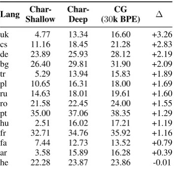
Table 3: BLEU scores (lowercased) comparing

character-level models against CG when used on30k BPE sequences. We show that without sweeping BPE, CG generally outper-forms purely character-level methods, even when the purely character-level networks are deepened as was shown to help in Cherry et al. (2018).

of 80 for our main experiments. At the end of each epoch we checkpoint and evaluate our model on a validation datset and used validation accuracy as our model selection criteria for test time. During decoding, a beam size of5 was chosen for all the experiments.

5.3 Results

target sequences and finally, (iii) against a purely character-level model.

5.3.1 BPE Results

Part1of Table 2 compares the best BLEU score obtained by the baseline model, after performing a BPE sweep from1.6k to60k, to the best BLEU obtained by CG after sweeping over the same BPE range. While our study focuses on the target side, BPE (with the same number of merge operations) was applied to both source and target for our ex-periments. We find that after this sweep, CG out-performs the baseline in all 14 languages. The ex-haustive table of results for these experiments is presented in Appendix A.

No Typical BPE Setting

Additionally, we see that the BPE setting that achieves best BLEU in the baseline model varies considerably from 1.6k to 30k depending on the target language, indicating that there is no “typ-ical” BPE for low-resource settings. In the CG model, however, performance was usually best at 30k. Part 2of Table 2 compares the baseline and CG at BPE of30k where CG performs optimally.

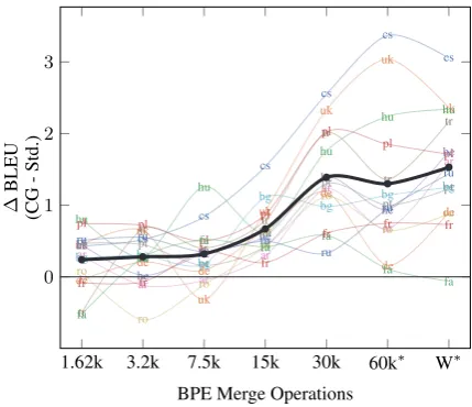
We find that our CG model consistently out-performs the baseline for almost all BPE merge hyperparameters across all 14 languages. Fig-ure 2 shows the gains observed by the CG model as we sweep over BPE merge operations. While the baseline model does slightly better than CG at small BPE settings for a few languages (all points below the0value), a majority of the points show positive gains.

5.3.2 Word-Level Results

In Part 3 of Table 2 we show results with our approximation for word level. While our best re-sults are generally with BPE, we note that we get the biggest relative gains using our method at the word level, which we expect is due to always hav-ing the whole word to learn character patterns over. For the CG model, in60k BPE and word-level set-tings we used the large vocabulary approximation discussed in Section 4.2.

5.3.3 Character-Level Results

Finally, in Table 3, we compare two character-level models against our CG model at 30k BPE. The shallow character-level model used 2 en-coder and deen-coder layers with1000recurrent units, while the deep model used6encoder and decoder

1.62k 3.2k 7.5k 15k 30k 60k∗ _W∗

0 1 2 3 cs cs cs cs cs cs cs uk uk uk uk uk uk uk hu hu hu hu hu hu hu pl pl pl pl pl pl pl he he he he he he he tr tr tr tr tr tr tr ar ar ar ar ar ar ar pt pt pt pt pt pt pt ro ro ro ro ro ro ro bg bg bg bg bg bg bg ru ru

ru ru ru ru ru de de de de de de de fa fa

fa _fa fa

fa fa

fr fr fr

fr

fr fr fr

BPE Merge Operations

∆

BLEU

(CG

-Std.)

Figure 2: Plot of the difference between the BLEU scores

from CG model and baseline model at various BPE settings for each of the14languages (shown in color, with language identifier). The bold black line shows the average difference across the languages for each BPE setting.

Features dependentCorpus- independent

Corpus-TT A H UT UTC

Correlation 0.04 0.59 0.67 0.80 0.49

Table 4: The Pearsons correlation between the features and

the relative gain in BLEU obtained by the CG model. See Section 6 for details regarding features.

layers with512recurrent units .7Furthermore, the improved results from the deep model were only attainable using the Fairseq toolkit with Noam op-timization and 100warmup steps (Gehring et al., 2017). As Table 3 shows, our CG model with30k BPE compares favorably to even deep character-level models for this low-resource setting.

6 Analysis

We are interested in understanding whether our character-aware model is exploiting morphologi-cal patterns in the target language. We investi-gate this by inspecting the relationship between a set of hand-picked features and improvements ob-tained by our model over the baseline at word-level inputs. These features fall into two cate-gories,corpus-dependentandcorpus-independent. We following Bentz et al. (2016), and extract fea-tures known to correlate with human judgments of morphological complexity. The following corpus-dependent features were used:

7_{Increasing the recurrent size for deep models resulted in}

(i) Type-Token Ratio (TT): the ratio of the num-ber of word types to the total numnum-ber of word tokens in the target side. We note that a large corpus tends to have a smaller type-token ra-tio compared to small corpus.

(ii) Word-Alignment Score (A): computed as A = |many-to-one_{|all-alignments}|−|one-to-many_| |. One-to-one, one-to-many and many-to-one alignment types are illustrated in Figure 3.8 _We

in-tuit that a morphologically poor source lan-guage (like English) paired with a richer tar-get language should exhibit more many-to-one alignments—a single word in the target will contain more information (via morpho-logical phenomena) that can only be trans-lated using multiple words in the source.

(iii) Word-Level Entropy (H): computed as_P H =

v∈Vp(v) logp(v) wherev is a word type.

This metric reflects the average information content of the words in a corpus. Languages with more dependence on having a large num-ber of word types rather than word order or phrase structure will score higher.

s1

s0 s2 s3 s4

t1

t0 t2 t3

Figure 3:Example of one-to-many (s0tot0, t1), one-to-one

(s1tot2) and many-to-one (s2, s3, s4tot3) alignments. For this exampleA= (3−2)/6.

For the corpus-independent features we used a morphological annotation corpus called Morph (Sylak-Glassman et al., 2015). The Uni-Morph corpus contains a large list of inflected words (in several languages) along with the word’s lemma and a set of morphological tags. For example, the French UniMorph corpus contains the wordmarchai(walked), which is associated with its lemma, marcherand a set of morpho-logical tags {V,IND,PST,1,SG,PFV}. There are19 such tags in the French UniMorph corpus. A morphologically richer language like Hungar-ian, for example, has 36 distinct tags. We used the number of distinct tags (UT) and the number of different tag combinations (UTC) that appear in the UniMorph corpus for each language. Note that 8_{We use FastAlign (Dyer et al., 2013) for word alignments}

with the grow-diag-final-and heuristic from (Och and Ney, 2003) for symmetrization.

we do not filter out words (and its associated tags) from the UniMorph corpus that are absent in our parallel data. This ensures that the UT and UTC features are completely corpus independent.

The Pearson’s correlation between these hand-picked features and relative gain observed by our model is shown in Table 4. For this analysis we used the relative gain obtained from the word-level experiments. Concretely, the relative gain for Czech was computed as 21.49−18.44

18.44 We see a

strong correlation between the corpus-independent feature (UT) and our model’s gain. Alignment score and Word Entropy are also moderately corre-lated. Surprisingly, we see no correlation to type-token ratio.

As the correlation analysis only examines the re-lation between BLEU gains and anindividual fea-ture, we further analyzed how the features jointly relate to BLEU gains. We fitted a linear regression model, setting the relative gains as the predicted variableyand the feature values as the input vari-ables x, with the goal of studying the linear

re-gression weightsφ.9 We used feature-augmented

domain adaptation where we consider each lan-guage as a domain (Daum´e III, 2007), allowing the model to find a set of “general” weights as well language-specific weights that best fit the data (Equation 11). The general feature weights can be interpreted as being indicative of the overall trends in the dataset across all the languages, while the language-specific weights indicate language devi-ation from the overall trend.

L(φ) =X

i∈I

|yi−y˜i |2 −λ|φ|2 (10)

˜

yi=φTALLxi+φTi xi (11)

Where,yis the true relative gain in BLEU,y˜is the predicted gain,xis a vector of input feature values,

φ_ALLandφ_iare the general and language-specific

weights, andiindexes into the set of languages in our analysis. We setλto0.05.

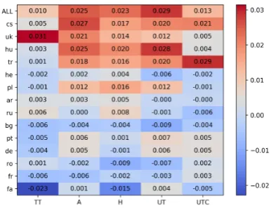
The matrix of learned weights φ is visualized

in Figure 4. The first row of weights correspond to the “general” weights that are used for all the languages, followed by language-specific weights sorted by relative gain.

While the general weights align with the corre-lation results (Table 4), this analysis also shows that the UTC weight for Czech and Turkish are 9_{The input features were min-max normalized for the}

Figure 4:Feature weights of the feature-augmented language adapted linear regression model. The first row represents the “general” set of weights used for all of the languages. Each row below are the language-adapted weights that only “fire” for that specific language.

much larger than any of the other languages’ and indeed we can verify that these languages have194 and300different tag combinations while the aver-age tag combinations is≈110.

From the corpus-dependent features, word alignment score strongly predicts the gain in BLEU scores. For Czech, Ukrainian, Turkish, Hungarian, and Polish we see additional weight placed on this feature. A similar trend can be seen for the word-entropy feature. While type-token ra-tio does not exhibit a strong overall trend, we see that Ukrainian and Farsi are outliers.

Our correlation and regression analysis strongly suggest that CG character-aware modeling helps the most when the target language has inherent morphological complexity and that it does indeed have the ability to handle morphological patterns present in the target languages.

6.1 Qualitative Examples

We additionally look at specific examples of where our model is outperforming the baseline in the case of30k BPE in En-Ar. We see a few trends, which we show examples of in Table 5. The first trend, corresponding to the first example, is that it gets names better. This might be because Arabic is not written in the Latin alphabet, and the spelling-aware model may be able to transliterate better.

Another trend is that CG gets the endings of rare words correct, in particular when the BPE seg-mentation is not according to morpheme bound-aries. The second example illustrates this, where the word for “Mexican” appears in the training data broken up by BPE with various morpholog-ical endings, all of which are spelled beginning

Src here he is : leonardoda vinci. Ref h*A hw – lywnArdwdA fyn$y. Std hnA hw : lywnArdwdA dA. CG hnA hw : lywnArdwdA fy+n$y. Src i ’m themexicanin the family .

Ref AnAAlmksykyfy AlEA}lp .

Std AnAmksy+Anyfy AlEA}lp .

CG AnAAlmksy+kyfy AlEA}lp .

Src there was going to be a nationalreferendum. Ref wtm AlAEdAd lAHrA’AstftA’$Eby . Std sykwn hnAkf+tA’wTny .

CG sykwn hnAkAst+f+tA’wTny . Src there are ordinaryheroes. Ref fhnAkAbTAlTbyEywn .

Std hnAkASdqA’EAdy .

CG hnAkAbTAlEAdyyn .

Table 5:Examples from En-Ar, transliterated with the

Buck-walter schema. We show the version of our model and the English using ‘+’ to denote where BPE splits words up, while BPE has not been applied to the target reference.

with “ky” in the second subword. The morpheme boundaries here would be “Al+mksyk+y.” Note that CG also gets the definite article “Al” correct while the baseline does not.

Finally, we see a pattern where our model does better for words which are rare and appear both with and without the definite article “Al.” Our third example in Table 5 illustrates this with an in-frequent word, the word for “referendum”, which gets broken up into subwords. In particular, the first subword sometimes has an “Al” attached in the training data. Our model is able to translate this subword, while the baseline skips the subword altogether, outputting two subwords that alone are not a valid word. Again, the word is not bro-ken up along morpheme boundaries by BPE. Here there would be no way to break this word up into morphological segments—it consists of non-concatenative derivational morphology. This oc-curs again in the fourth example in the word for “heroes,” where the baseline predicts the word for “friends.” In this case the word was not split up by BPE, but similarly it is rare but occurs with the definite article attached in the training data as well.

7 Conclusion

translating from English into 14 languages, and on top of a spectrum of BPE merge operations. Fur-thermore, for word-level and higher merge hyper-parameter settings, we introduced an approxima-tion to the softmax layer. We achieve consistent performance gains across languages and subword granularities, and perform an analysis indicating that the gains for each language correspond to mor-phological complexity.

For future work, we would like to explore how our methods might be of use in higher-resource settings. Furthermore, it would be interesting to see how these methods might interact with multi-lingual systems and if they might be able to im-prove what information is shared between related languages.

Acknowledgements

This project originated at the Machine Translation Marathon 2018. We thank the organizers and at-tendees for their support, feedback and helpful dis-cussions during the event. This work is supported in part by the Office of the Director of National In-telligence, IARPA. The views contained herein are those of the authors and do not necessarily reflect the position of the sponsors.

References

Bahar, Parnia, Tamer Alkhouli, Jan-Thorsten Peter, Christopher Jan-Steffen Brix, and Hermann Ney. 2017. Empirical investigation of optimization algo-rithms in neural machine translation. The Prague Bulletin of Mathematical Linguistics, 108(1):13–25.

Bahdanau, Dzmitry, Kyunghyun Cho, and Yoshua Ben-gio. 2015. Neural machine translation by jointly learning to align and translate. International Con-ference on Learning Representations.

Belinkov, Yonatan, Nadir Durrani, Fahim Dalvi, Has-san Sajjad, and James Glass. 2017. What do neu-ral machine translation models learn about morphol-ogy? InProceedings of the 55th Annual Meeting of the Association for Computational Linguistics (Vol-ume 1: Long Papers), pages 861–872. Association for Computational Linguistics.

Bentz, Christian, Tatyana Ruzsics, Alexander Ko-plenig, and Tanja Samardzic. 2016. A comparison between morphological complexity measures: typo-logical data vs. language corpora. InProceedings of the Workshop on Computational Linguistics for Lin-guistic Complexity (CL4LC), pages 142–153.

Cettolo, Mauro, Christian Girardi, and Marcello Fed-erico. 2012. Wit3: Web inventory of transcribed and

translated talks. InConference of European Associ-ation for Machine TranslAssoci-ation, pages 261–268. Cherry, Colin, George Foster, Ankur Bapna, Orhan

Firat, and Wolfgang Macherey. 2018. Revisiting character-based neural machine translation with ca-pacity and compression. InProceedings of the 2018 Conference on Empirical Methods in Natural Lan-guage Processing, pages 4295–4305.

Chung, Junyoung, Kyunghyun Cho, and Yoshua Ben-gio. 2016. A character-level decoder without ex-plicit segmentation for neural machine translation. InProceedings of the 54th Annual Meeting of the As-sociation for Computational Linguistics (Volume 1: Long Papers), pages 1693–1703.

Costa-juss`a, Marta R and Jos´e AR Fonollosa. 2016. Character-based neural machine translation. In Pro-ceedings of the 54th Annual Meeting of the Associa-tion for ComputaAssocia-tional Linguistics (Volume 2: Short Papers), pages 357–361.

Daum´e III, Hal. 2007. Frustratingly easy domain adap-tation. InProceedings of the 45th Annual Meeting of the Association of Computational Linguistics, pages 256–263, June.

Duh, Kevin. 2018. The multitarget ted talks task. http://www.cs.jhu.edu/˜kevinduh/a/ multitarget-tedtalks/.

Dyer, Chris, Victor Chahuneau, and Noah A Smith. 2013. A simple, fast, and effective reparameteriza-tion of ibm model 2. In Proceedings of the 2013 Conference of the North American Chapter of the Association for Computational Linguistics: Human Language Technologies, pages 644–648.

Gage, Philip. 1994. A new algorithm for data compres-sion.C Users J., 12(2):23–38, February.

Gehring, Jonas, Michael Auli, David Grangier, Denis Yarats, and Yann N Dauphin. 2017. Convolutional Sequence to Sequence Learning. ArXiv e-prints, May.

Jean, S´ebastien, Kyunghyun Cho, Roland Memisevic, and Yoshua Bengio. 2015. On using very large tar-get vocabulary for neural machine translation. In

Proceedings of the 53rd Annual Meeting of the As-sociation for Computational Linguistics and the 7th International Joint Conference on Natural Language Processing (Volume 1: Long Papers), pages 1–10. Kim, Yoon, Yacine Jernite, David Sontag, and

Alexan-der M Rush. 2016. Character-aware neural language models. In30th AAAI Conference on Artificial Intel-ligence, AAAI 2016.

Ling, Wang, Isabel Trancoso, Chris Dyer, and Alan W Black. 2015. Character-based neural machine trans-lation. arXiv preprint arXiv:1511.04586.

Luong, Thang, Hieu Pham, and Christopher D. Man-ning. 2015. Effective approaches to attention-based neural machine translation. In Proceedings of the 2015 Conference on Empirical Methods in Natural Language Processing, EMNLP 2015, Lisbon, Portu-gal, September 17-21, 2015, pages 1412–1421. Maruf, Sameen and Gholamreza Haffari. 2018.

Docu-ment context neural machine translation with mem-ory networks. In Proceedings of the 56th Annual Meeting of the Association for Computational Lin-guistics (Volume 1: Long Papers), volume 1, pages 1275–1284.

Miyamoto, Yasumasa and Kyunghyun Cho. 2016. Gated word-character recurrent language model. In

Proceedings of the 2016 Conference on Empirical Methods in Natural Language Processing, pages 1992–1997.

Och, Franz Josef and Hermann Ney. 2003. A system-atic comparison of various statistical alignment mod-els. Computational linguistics, 29(1):19–51.

Passban, Peyman, Qun Liu, and Andy Way. 2018. Im-proving character-based decoding using target-side morphological information for neural machine trans-lation. In Proceedings of the 2018 Conference of the North American Chapter of the Association for Computational Linguistics: Human Language Tech-nologies, Volume 1 (Long Papers), volume 1, pages 58–68.

Sennrich, Rico, Barry Haddow, and Alexandra Birch. 2016. Neural machine translation of rare words with subword units. InProceedings of the 54th Annual Meeting of the Association for Computational Lin-guistics, ACL 2016, August 7-12, 2016, Berlin, Ger-many, Volume 1: Long Papers.

Shapiro, Pamela and Kevin Duh. 2018. Bpe and charcnns for translation of morphology: A cross-lingual comparison and analysis. arXiv preprint arXiv:1809.01301.

A More Detailed Results

In Table 6, we provide the number of training sen-tences for each language.

Language Number of sentences

Czech (cs) 81k

Ukrainian (uk) 74k

Hungarian (hu) 108k

Polish (pl) 149k

Hebrew (he) 181k

Turkish (tr) 137k

Arabic (ar) 168k

Portuguese (pt) 147k

Romanian (ro) 155k

Bulgarian (bg) 159k

Russian (ru) 174k

German (de) 146k

Farsi (fa) 106k

French (fr) 149k

Table 6:Number of sentences in training data for each language

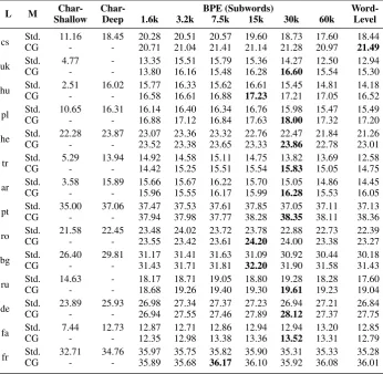
L M _ShallowChar- Char-_{Deep 1.6k 3.2k} BPE (Subwords)_{7.5k 15k 30k 60k} Word-_Level

cs Std._CG 11.16_- 18.45_- 20.28_{20.71 21.04}20.51 20.57_21.41 19.60_{21.14 21.28}18.73 _20.9717.60 18.44_21.49

uk Std._CG 4.77_- -_- 13.35_{13.80 16.16}15.51 15.79_15.48 15.36_{16.28 16.60}14.27 _15.5412.50 12.94_15.30

hu Std._CG 2.51_- 16.02_- 15.77_{16.58 16.61}16.33 15.62_16.88 16.61_{17.23 17.21}15.45 _17.0514.81 14.18_16.52

pl Std._CG 10.65_- 16.31_- 16.14_{16.88 17.12}16.40 16.34_16.84 16.76_{17.63 18.00}15.98 _17.3215.47 15.49_17.20

he Std._CG 22.28_- 23.87_- 23.07_{23.52 23.38}23.36 23.32_23.65 22.76_{23.33 23.86}22.47 _22.7821.84 21.26_23.01

tr Std._CG 5.29_- 13.94_- 14.92_{14.42 15.25}14.58 15.11_15.51 14.75_{15.54 15.83}13.82 _15.0513.69 12.58_14.75

ar Std._CG 3.58_- 15.89_- 15.66_{15.96 15.55}15.67 16.22_16.17 15.70_{15.99 16.28}15.05 _15.5314.86 14.45_16.05

pt Std._CG 35.00_- 37.06_- 37.47_{37.94 37.98}37.53 37.61_37.77 37.85_{38.28 38.35}37.05 _38.1137.11 37.13_38.36

ro Std._CG 21.58_- 22.45_- 23.48_{23.55 23.42}24.02 23.72_23.61 23.78_{24.20 24.00}22.88 _23.3822.73 22.39_23.27

bg Std._CG 26.40_- 29.81_- 31.17_{31.43 31.71}31.41 31.63_31.81 31.09_{32.20 31.90}30.92 _31.5830.44 30.18_31.43

ru Std._CG 14.63_- -_- 18.17_{18.68 19.26}18.71 19.05_19.40 18.80_{19.30 19.61}19.28 _19.2318.28 17.60_19.04

de Std._CG 23.89_- 25.93_- 26.98_{26.94 27.55}27.34 27.37_27.46 27.23_{27.89 28.12}26.94 _27.3727.21 26.84_27.75

fa Std._CG 7.44_- 12.73_- 12.87_{12.35 12.98}12.71 12.86_13.38 12.94_{13.36 13.52}12.94 _13.3113.20 12.85_12.79

fr Std._CG 32.71_- 34.76_- 35.97_{35.89 35.68}35.75 35.82_36.17 35.90_{36.10 35.92}35.31 _36.0835.33 35.28_36.01

Table 7:BLEU scores (case insensitive) for a standard embedding encoder-decoder baseline (Std), and character-aware model,