Scouting Context sensitive Components

Scouting Context-sensitive Components

Jeffrey O. Pfaffmann and Klaus-Peter Zauner

Department of Computer Science

Wayne State University

Detroit, Michigan, 48201, U.S.A.

[email protected]

fax.: +313-577-6868, ph.: +313-577-2477

In D. Keymeulen, A. Stoica, J. Lohn, and R. S. Zebulum, editors, The Third NASA/DoD Workshop on Evolvable Hardware—EH-2001, Long Beach, 12–14 July 2001. IEEE Computer Society, Los Alamitos, pp. 14–20, 2001.

Abstract

Nature’s gadgets are implemented without being planned and therefore can utilize context-sensitive com-ponents. Thus functionality that would require extensive networks of context-free components can be elicited from a minimum of material. Proteins can serve as context-sensitive components for pattern processing applications. We here describe an evolutionary search strategy currently under investigation for its potential use in conjunction with computer controlled f luidics to evaluate the computational capabilities of proteins. Our algorithm employs evolution-ary search not to seek an optimum, but to seek surprises. It directs experiments and incrementally constructs an empir-ical model from their outcome. Reward is given for discov-ering conditions that exhibit a discrepancy between the pre-diction of the current model and the experimental result. As unexpected observations are incorporated into the model, the reward associated with them vanishes. Results obtained so far indicate that evolutionary search is a useful paradigm for characterizing the phenomenology of context-sensitive components.

1. Introduction

Eugene Wigner once remarked that “[. . . ] the construc-tion of machines, the funcconstruc-tion of which he can foresee, con-stitutes the most spectacular accomplishment of the physi-cist” [27]. The engineering approach in which mental con-ception precedes physical creation is extremely efficient, but at the same time severely limited by our capacity to predict the behavior of artifacts. If prediction is not fea-sible, however, engineering often proceeds with an essen-tially evolutionary approach. The early history of optical engineering is a case in point [11].

Prediction is computation. A physical system can be viewed as computing its own behavior and might be the

most effective architecture to do so. Whenever the predic-tion of the system’s behavior is harder than the implemen-tation and evaluation of the system itself, evolution may provide the shortest path to a system design that satisfies given requirements. In a planned design the requirements are used to instruct the construction or modification of the system. Evolution, on the contrary, creates a population of arbitrarily constructed or modified systems and applies the requirements to select a subset of the population for further modification. Thus evolution uses the implementation of a system (parent) to estimate the performance of arbitrarily modified versions of this system (offspring). The evolution-ary engineering paradigm is not only capable of coping with self-organizing, globally interacting systems, but is particu-larly effective in this domain (cf. [24, 26]).

The instructive use of the requirements for systems de-sign is so familiar to human thought, that it is often assumed as the first explanation for any seemingly purposeful design. Nature, however, utilizes evolution’s selective paradigm on many different levels of scale. The design of species in ecosystems and of antibodies in the immune system are ex-amples where the initial assumption of an instructive pro-cess gave way to an explanation based on a selective propro-cess [10]. It appears that conformational state transitions in en-zymatic catalysis could be the next process whose explana-tion will undergo this shift from an instructive to a selective paradigm [17].

The key point that makes evolution attractive from the technological perspective is its reliance on arbitrary rather than directed system modifications. Since evolution does not depend on a predictable relationship between a given modification and system performance it can cope with nu-merous interacting factors and with situations for which mechanistic models are either not available or so complex as to be impractical [3]. This led to the idea of ‘automatic research machines’ that can search for ideal parameter set-tings in real world physical devices [20]. Random changes to the parameters are accepted (or rejected) if the new

rameter settings reduce (or increase) the distance to the de-sign goal.

Evolutionary experimentation thus resembles the ap-proach of a craftsman who does not theorize about his work but nevertheless achieves a high degree of perfection through constant feedback from interaction with the ‘hard-ware’ of his craft. The scouting algorithm described below is an attempt to capture another aspect of the craftsman’s approach—the curiosity of his mind directing his attention to unexpected observations, free of any particular design goal. The potential significance of the observations can sub-sequently be contemplated with the aid of human creativity.

1.1. The role of context-sensitive components

The concept of scouting has been developed as a tool to identify behavior of context-sensitive components that may be exploited in computing devices. Components are context-sensitive if their function cannot be described with-out taking the system which they are part of into consider-ation. Such components are an invaluable source of com-plexity for the implementation of pattern processors [30].

Complexity is a computational resource because the al-gorithmic complexity (K) of the input-output behavior (f) of an information processor can never exceed the combined complexity of the processor’s architecture (a) and of the program (pf) that specifies the behavior of the processor:

K(f)≤ K(a) +K(pf)

This follows directly from the definition of algorithmic complexity [4, 13, 25]: K(f)corresponds to the length of the shortest description sufficient to generatef. Since the programpf in combination with a machine of architecture

ais able to generatef, a description ofpf together with a

description ofaconstitutes a description of f. Hence the shortest way to describef cannot be longer than the com-bination of the shortest descriptions ofpf anda. Since

al-most all possible mapsf have high algorithmic complexity

K(f)—a consequence of the fact that there are more input-output tables than descriptions that would be shorter than the tables—the low complexity K(a) of the conventional machine architectures makes programs of formidable com-plexityK(pf)inevitable.

Consider, for example, the simple 10×10 bit pattern (100 bit input) shown in Fig. 1. There are22100

possible clas-sifications of the input patterns into two groups (1 bit out-put) such as ‘accept’ and ‘reject’. A program that would implement an arbitrary one of these seemingly simple map-pings is likely to be so long that it is entirely impractical. Correspondingly, a specialized hardware architecture built from simple components could require a very large num-ber of them. The use of context-sensitive components and their concomitant complex interactions may open up a path

for implementing high-complexity pattern processors with significantly less hardware than conventional technologies require.

10 × 10 n = 100 bits

p

I

Yes/No m = 1 bit

O

O=f(I)

a

Figure 1. Pattern classification with a general purpose computer. The program pf has to

select the desired classification map f from the set of all possible system behaviors.

Conceivably, nature’s molecular information processors employ context-sensitive components to efficiently imple-ment complex computing operations. Moreover, biological systems allow for molecular self-organization to dynami-cally reconfigure their processing architecture [16].

1.2. Signal processing wetware

inversion [12, 18, 19].

In the early 1970s the idea of considering biological structures as natural molecular computers came up [5, 14]. Subsequently numerous schemes for utilizing biomolecules in artificial information processing devices came into con-sideration (e.g., [1, 2, 9]).

The use of macromolecules for information processing poses a problem in which the sought resource, molecular level interactions, goes hand in hand with the impracticality of foretelling system behavior [6, 7]. This is particularly the case for proteins. As context-sensitive components they are refractory to simple mechanistic modeling but can be characterized empirically [29]. The challenge is to map out component response with respect to numerous interacting factors, and to do so with a limited number of experimental tests.

Fig. 2 shows the computer controlled fluidics of a setup developed to characterize the response of enzymes (i.e., cat-alytically active proteins) to various milieu conditions. This

c °Zauner

Figure 2. Computer controlled fluidics devel-oped for the automated exploration of pro-tein context-sensitivity. Sixteen servos (of the type used for radio controlled model air-planes) are employed to control 6 syringe pumps, 9 valves and a peristaltic pump (from [28]).

setup enables an evolutionary experimentation algorithm, running on a digital computer, to probe the response of en-zymes. The computer can compose a chemical milieu from up to five substances and then measure the catalytic activity of the enzyme in the milieu.

It would be possible to specify a desired signal process-ing behavior as the goal for the evolutionary experimen-tation and to use the setup as an ‘automatic research ma-chine’ of the type proposed by Rechenberg. However, to explore more generally the capabilities of proteins to serve as context-sensitive components in molecular devices, we are currently investigating the scouting algorithm described

A B1

C1

B2 C2

Figure 3. Random sampling vs. scouting. The phenomenon under investigation is repre-sented by a 100×100 pixel gray level image (A). Sampling 5% of A at random locations (B1) leads to estimate C1 of the phenomenon. Exploring A with the scouting algorithm di-rects the sample locations towards heteroge-neous areas and thus can acquire more de-tailed information with the same number of samples.

in the next section as a method of controlling the fluidics setup.

2. The scouting algorithm

The task of the scouting algorithm is the exploration of complex phenomena. To analyze and illustrate different scouting strategies we decided to emulate phenomena through gray-scale images. The xandy axes correspond to two factors with the gray values in the image plane repre-senting the response for specific factor levels. This method has the advantage that phenomena with arbitrary and com-plex features can conveniently be prepared. For simplicity the following discussion will assume that only two factors are considered (i.e., a two-dimensional factor space), but all operations extend to higher dimensions as will be required, for example, to drive the five-factor fluidics setup shown in Fig. 2.

Generally in this application the knowledge that can be acquired is limited by the number of experiments that can be conducted, not by available computing resources. It is desirable that the samples be distributed in the factor space for maximum information gain. Fig. 3 illustrates the fo-cusing of the sampling on detail rich areas that occurs with scouting.

Hypothesis

(fixed rule)

Phenomenon

(response)

Experience

(database)

Expectation

(x,r_')

Observation

Experiment

(specification) r = f(x)

x x

(surprise value) Evaluation

(x,r)

(x,r)

(x,r_') d(r,r_')

Evolution

Figure 4. Schematic view of the scouting algo-rithm. From a population of experiments, the specification (x) of the experiment that gave rise to the most surprising observation (x,r) in view of the current experience is selected for reproduction.

in the factor space, is subjected to evolution. For each in-dividual in the population first an expected response r0 _is

computed from the contents of the experience database us-ing a fixed hypothesis to extrapolate the known experiences. Then the phenomenon is probed for the conditionx result-ing in a responser. The observation(x, r)is compared to the expectation(x, r0_{). A large differenced(r, r}0_)between

expected and actual response, i.e., a surprising observation, is associated with a high fitness value for the individual that requested the observation. The observation (x, r) is also entered into the database of experiences and can con-tribute to the evaluation of the next individual. Every exper-iment performed on the phenomenon contributes to the ex-perience stored in the database and consequently leads to a refinement of the expectation. For all results presented here the population size was ten, all individuals being offspring of the single best individual selected for reproduction. Thus, the individuals live for one generation only. Their fitness would in any case be low after one generation; after they have been evaluated once there is experience available in the database for the factor combination which they repre-sent and subsequent experiments would not yield surprising observations (assuming no measurement errors).

Individuals are derived through random variation of the location in the factor space that the parent individual repre-sents. The magnitude of the variation is a function of the fitness of the parent. (Each factor is varied by a uniformly distributed pseudorandom amount less than±0.03 for a par-ent whose surprise valued(r, r0_{)was above 0.7, less than}

±0.04 ifd(r, r0_{)was above 0.2, less than±0.2 ifd(r, r}0₎

was above 0.05, and anywhere within the factor range

oth-erwise.)

It is important to note that the algorithm does not opti-mize factor levels with regard to some desired response. In-stead it rewards those individuals in the population that di-rect the search towards unexpected response behavior. The expectation is of course not constant and changes as infor-mation is acquired.

The expected response for all points in the factor space forms a model of the phenomenon and becomes more refined with each experiment. The factor levels as well as the response level are normalized (0 ≤x≤1,0≤y ≤1, 0 ≤r≤1). The expected response (r0_{) for a location}

xin the factor space is computed from the observations closest tox. If the database is empty, the expected response for any location in the factor space is set to 0.5 (the middle value of the normalized scale), if only one observation is in the database, the expected response for anyxis the same as the one observed response. In general a fixed maximum num-ber of observationsr(set to 10 for the runs reported here) is considered in the calculation of an expected responser0_.

G C A

E H

D

B F

I L_y

J 0.0

1.0 y

1.0

0.0 x

a

b

c d

e

d(a)

d(c) d(b)

L_x

x_s

y_{s s}

Figure 5. Deriving expectations from experi-ence. The observations (a–e) are each repre-sented in two lists (Lxand Ly) sorted

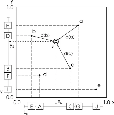
accord-ing to the x and y factor levels. The expected response at s is computed from the known responses of a set of observations nearest to s. See text for details.

factor space. Fig. 5 illustrates the two-dimensional case, assuming that five observations (labeled a–e in the £gure) have been entered into the experience database. The list Lx

represents the five observations sorted according to their x-factor levels and correspondingly Lyrepresents them sorted

according to their y-factor levels. To retrieve the observa-tions relevant to computing the expectation for the specified experiment s=(xs, ys), first the lower neighbor ofxsin Lx

is accessed (labeled A) and the corresponding observation d retrieved. For this example we assume that only three observations will be used to calculate the expected value. The distance of observation d from s in the factor space is computed and d entered into a list of potentially relevant observations ([d]). The entries in this list are maintained in sorted order with respect to their distance from s. Next, the lower neighbor of s in the next dimension (i.e., from Ly) is

considered and consequently observation c is added to the list of potentially relevant observations. Since c is closer to s than d is, it is inserted to the left of d ([c,d]). Subsequently the lists of all dimensions are traversed from the immediate neighbors of the point (xs, ys) outward and observations

added to the potentially relevant observations. After entry D in list Lyhas been considered the list of potentially

rele-vant observations contains [b,c,d].

If all positions in the list of potentially relevant observa-tions are filled, an observation will be sorted into the list if it is closer to s than the farthest observations in the list, the latter then being discarded. If an entry in Lxhas an x value

that is further fromxsthan the rightmost entry in the list of

potentially relevant observations, Lxis not further traversed

in this direction. Traversal is also stopped at the end of a list. Corresponding rules apply to both directions in all di-mensions. The entries remaining in the list of potentially relevant observations after list-traversal has stopped in all dimensions are then used to compute the expectation.

For the data presented we used in all cases the following hypothesis to derive the expectation from the relevant ob-servations. The observed response values are weighted by the cubic distance between the location of the observation and the specified factor space location. The weighted av-erage of the observed response values is then taken as the expected response.

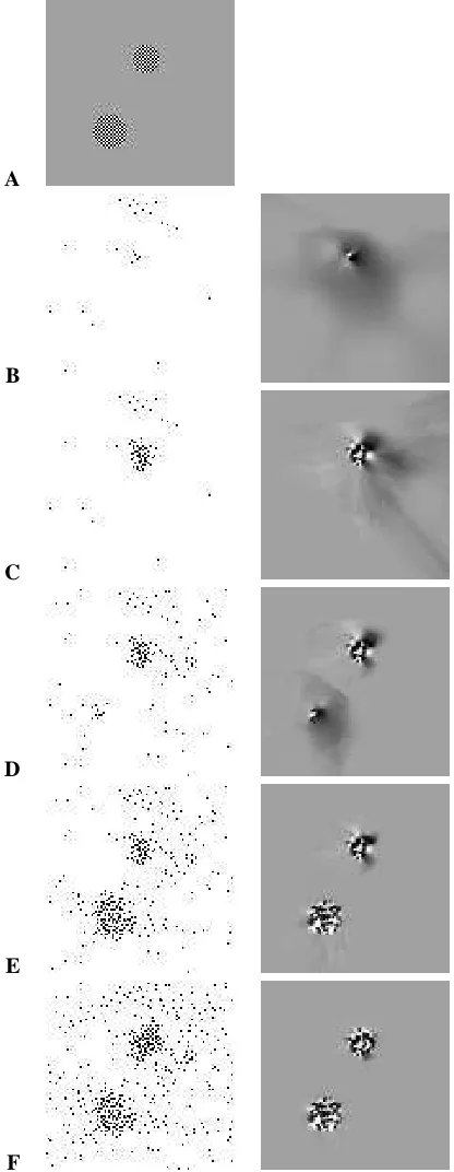
Fig. 6 illustrates the progress of the scouting algorithm’s sampling activity. The 100×100 pixel image representing the phenomenon is shown on the top left. It contains two spots of fine detail, that on average are very similar to the rest of the factor space. In rows B–F dots in the left square indicate the locations in the factor space where the phe-nomenon has been probed. The squares in the right column show the expected gray value for every location in the factor space, given the observations indicated in the left square. In combination they represent an empirical model of the phe-nomenon.

A

B

C

D

E

F

0 0.1 0.2 0.3 0.4 0.5 0.6 0.7 0.8 0.9 1

0 50 100 150 200 250 300 350 400 450 500

Suprise value

Observation

Figure 7. Differences between expected and observed values during the progress of the sampling shown in Fig. 6. The £rst burst cor-responds to the sampling of the upper spot, the second burst corresponds to the discov-ery of the lower spot.

Sampling starts at a random location in the factor space. In the example shown in Fig. 6, the £rst samples are taken in the top center. Because the phenomenon shows a uni-form response, only the first sample taken has some sur-prise value (being different from the 0.5 value assumed in the absence of any observations). Due to the low fitness of the parent selected from the first generation, the offspring shows broad variation in its factor levels and spreads in the factor space. Some individuals sample the area of fine detail in the upper center of the space. Unexpected observations from the factor combinations in this area yield high surprise values (shown in Fig. 7) and correspondingly high fitness for the individuals that discovered the area. The dark shad-ows visible in the right square of Fig. 6B, i.e., the model derived from the first 25 samples, attest to distant extrapo-lation in the sparsely sampled space.

As the population concentrates in the high fitness area, the experience in this area increases and consequently the expectations become more accurate. The decrease in sur-prise value leads to a wider spread in the population and to the possibility that a more interesting area of the space is discovered. After 14 generations the second detailed area in the factor space is discovered (Fig. 6D and the second burst in Fig. 7) and explored.

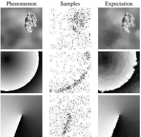
Fig. 8 shows the clustering of sampling at factor levels that give rise to abrupt response changes and the concomi-tant reduced sampling density at factor combinations that yield a graded response. Fig. 9 gives an impression of how much the sample clustering varies among different initial-izations of the pseudorandom generator.

Phenomenon Samples Expectation

Figure 8. Clustering of 500 sampling locations for different phenomena.

Figure 9. Sample locations of 500 samples for £ve different runs probing the same phe-nomenon.

3. Concluding remarks

areas of complex behavior and sparsely in areas that show less factor interaction.

The results we have obtained so far show that the com-bination of a very simple strategy for evolutionary experi-mentation with a simple empirical modeling of the response behavior suf£ces for sample clustering to occur in areas of high interest. These £ndings are based on the application of the algorithm to phenomena emulated by gray-scale im-ages, not to real world experiments. Further tests are re-quired to evaluate the performance of the scouting method under noise in both the response and the factor levels, be-fore it can usefully be applied in actual computer controlled experimentation.

Hardware evolution faces the dichotomy that only real physical implementations can harvest its full potency, but at the same time such implementations are impractical for any system short of a self-replicating one. Methods like scouting may be able to narrow the gap between simulation and experimentation as means for fitness evaluation.

Acknowledgements. We gratefully acknowledge the

dis-cussions with our teacher Michael Conrad before his death in December 2000. The reported material is based upon work supported by the U.S. National Science Foundation under Grant Nos. ECS-9704190 and CCR-9610054, and by NASA under Grant No. NCC2-1189, all to Michael Conrad.

References

[1] L. M. Adleman. Molecular computation of solutions to com-binatorial problems. Science, 266:1021–1024, 1994. [2] T. Aoki, M. Kameyama, and T. Higuchi.

Interconnection-free biomolecular computing. Computer (IEEE), 25:41–50, 1992.

[3] G. E. P. Box. Evolutionary operation: A method for increas-ing industrial productivity. Appl. Statist., 6:81–101, 1957. [4] G. J. Chaitin. Algorithmic information theory. IBM Journal

of Research and Development, 21:350–359,496, 1977.

[5] M. Conrad. Information processing in molecular systems.

Currents in Modern Biology (now BioSystems), 5:1–14,

1972.

[6] M. Conrad. On design principles for a molecular computer.

Commun. ACM, 28:464–479, 1985.

[7] M. Conrad and H. M. Hastings. Scale change and the emer-gence of information processing primitives. J. theor. Biol., 112:741–755, 1985.

[8] A. Hjelmfelt and J. Ross. Mass-coupled chemical systems with computational properties. J. Phys. Chem., 97:7988– 7992, 1993.

[9] F. T. Hong. The bacteriorhodopsin model membrane system as a prototype molecular computing element. BioSystems, 19:223–236, 1986.

[10] N. K. Jerne. Antibody and learning: Selection versus in-struction. In G. C. Quarton, T. Melnechuk, and F. O. Schmitt, editors, The Neurosciences, pages 200–205. Rock-efeller University Press, New York, 1967.

[11] R. Kingslake. The development of the photographic objec-tive. J. Optical Society of America, 24:73–84, 1934. [12] L. Kuhnert, K. I. Agladze, and V. I. Krinsky. Image

process-ing usprocess-ing light-sensitive chemical waves. Nature, 337:244– 247, 1989.

[13] M. Li and P. Vit´anyi. An Introduction to Kolmogorov

Com-plexity and its Applications. Springer, New York, 2nd

edi-tion, 1997.

[14] E. A. Liberman. Cell as a molecular computer (MCC).

Bio£zika, 17:932–943, 1972.

[15] F. R. Pettit. Post-Digital Electronics, chapter 13, pages

161,162,165. Electrical and Electronic Engineering. Ellis Horwood, Chichester, West Sussex, 1982.

[16] J. O. Pfaffmann and M. Conrad. Adaptive information pro-cessing in microtubule networks. BioSystems, 55:47–58,

2000.

[17] S. D. Rader and D. A. Agard. Conformational substates in enzyme mechanism: the 120K structure ofα-lytic protease at 1.5 ªa resolution. Protein Sci., 6:1375–1386, 1997. [18] N. G. Rambidi. Nondiscrete biomolecular computing.

Com-puter (IEEE), 25:51–54, 1992.

[19] N. G. Rambidi and A. V. Maximychev. Towards a biomolecular computer: information processing capabili-ties of biomolecular nonlinear dynamic media. BioSystems, 41:195–211, 1997.

[20] I. Rechenberg. Cybernetic solution path of an experimental problem. Technical report, Royal Aircraft Establishment, Library Translation 1122, Farnborough, 1965. Reprinted with commentary in D. B. Fogel, editor, Evolutionary

Com-putation: The Fossil Record, pages 297–309, IEEE Press,

New York, 1998.

[21] O. E. R¨ossler. Chemical automata in homogeneous and reaction-diffusion kinetics. In M. Conrad, W. G ¨uttinger, and M. D. Cin, editors, Physics and Mathematics of the Nervous

System, volume 4 of Lecture Notes in Biomathematics, pages

399–418. Springer, Heidelberg, 1974.

[22] S. K. Scott. Oscillations, waves and chaos in chemical

ki-netics. Oxford University Press, Oxford, 1994.

[23] F. F. Seelig and O. E. R ¨ossler. A chemical reaction ¤ip-¤op with one unique switching input. Zeitschrift f ¨ur

Natur-forschung, 27b:1441–1444, 1972.

[24] J. L. Segovia-Juarez and S. Colombano. Mutation buffer-ing capabilities of the hypernetwork model. In the present volume, 2001.

[25] R. J. Solomonoff. A formal theory of inductive inference.

Information and Control, 7:1–22, 224–254, 1964.

[26] L. G. Volkert and M. Conrad. The role of weak interactions in biological systems: the dual dynamics model. J. theor.

Biol., 193:287–306, 1998.

[27] E. P. Wigner. The unreasonable effectiveness of mathemat-ics in the natural sciences. Comm. Pure. Appl. Math., 13:1– 14, 1959.

[28] K.-P. Zauner. Conformation-based Molecular Computing:

Simulation and Implementation. PhD thesis, Wayne State

University, Detroit, Michigan, 2001.

[29] K.-P. Zauner and M. Conrad. Enzymatic pattern processing.

Naturwissenschaften, 87(8):360–362, 2000.