Bootstrap Based Bilateral Smoothing of Point Sets
Ahmad Ramli, Nor Aziyatul Izni Mohd Rosli and Ioannis Ivrissimtzis
Abstract—Boostrap is a statistical method widely used in applications such as model averaging and noise estimation. In this paper, we propose a bilateral smoothing algorithm based on bootstrap noise estimates for denoising 3D point sets. Following a classic denoising technique, for a given neighbourhood of the point set, we first fit a polynomial surface and then update the position of each point of the neighbourhood by moving it towards its projection on the fitted surface. However, in the proposed algorithm, the amount by which we move each vertex towards its projection depends on the bootstrap error estimate of the polynomial fitting. As a result, low quality polynomial fittings with high bootstrap error estimates tend have smaller effect on the denoising process and do not degrade the final result. We also propose a multi-pass, density adaptive variant of the proposed bilateral smoothing and experimentally show that it can further improve the results.
Index Terms—surface reconstruction, points set smoothing, bilateral filtering, bootstrap.
I. INTRODUCTION
I
N the pipeline of surface reconstruction, we start with a set of unorganised 3D points, usually obtained from a 3D laser scanner or extracted from a set of images, and we compute a surface modelling this point set. The reconstructed surface may be a polygonal mesh, or a free-form surface such as NURBS, or even a point set surface, that is, be represented by the point set itself. Regardless of the representation of the reconstructed surface, it is quite common that the initially acquired point set will need to be denoised in a pre-processing step, typically by applying a point set smoothing algorithm on it.In this paper, we propose a point set smoothing algorithm based on bilateral filtering. The algorithm moves each point P of a neighbourhood of the point set towards the average of the projections of P on bootstrap polynomial fittings of the neighborhood, or, in other words, updates P as a linear combination of itself and the average of the projections on the bootstrap fittings. Being a bilateral smoothing algorithm, the weight of the linear combination, which indicates the amount of smoothing received by P, depends on two independent parameters. The first is a the distance of P from the centre of the neighborhood, with points further away receiving less smoothing. The second parameter is the bootstrap error estimate for the polynomial fittings, with high error estimates reducing the amount of smoothing and thus, blocking bad polynomial fittings out of the smoothing process.
Finally, in Section IV, we discuss a multi-pass variant of the proposed algorithm, which also adapts the size of the considered neighbourhoods to an estimate of the local density of the point set.
Manuscript received March 17, 2013; revised April 15, 2013.
Ahmad Ramli and Nor Aziyatul Izni Mohd Rosli are with the School of Mathematics, Universiti Sains Malaysia, e-mail: [email protected]
Ioannis Ivrissimtzis is with Durham University.
II. RELATEDWORK
Bootstrap is a model averaging technique proposed by Efron [1]. Given a datasetPof sizeN, one createsBsubsets ofPby randomly samplingNelements ofPwith repetition. The repetition in the sampling process means that we usually sample less thanN distinct elements and thus, the bootstrap subsets are proper subsets ofP. Bootstrap modelling, fits a model on bootstrap subset and computes an average model. Bootstrap error estimation analyses the bootstrap models and uses the leftover data in the complement of each subset inP to compute an error estimate for the average bootstrap model. A detailed description of bootstrap and a discussion of its properties can be found in standard textbooks on statistical learning such as [2].
Cabrera and Meer [3] applied bootstrap on a 2-dimensional setting. In [4], we used bootstrap to obtain error estimates on 3D point sets. We also presented a naive smoothing algorithm which projected the points towards their projection on bootstrap polynomial fittings. The results there were limited by the simplicity of the projection used.
Data smoothing can be integrated into the reconstruction algorithm as, for example, in the implicit reconstruction algorithm proposed in [5]. However, most smoothing ap-proaches are forms on data filtering and can be used as a pre-processing step, independently of the reconstruction. In particular, adapting the approach that originated in image denoising [6], one may smooth noisy 3D data using bilateral filtering.
Fleishman et al. [7] and Jones et al. [8] adapted bilateral image filtering for triangle mesh smoothing. In Fleishman et al. [7], the first parameter of the filter penalises the distance of the point from the centre of the neighbourhood, while the second parameter penalises the difference between the normal of the point and the normal at the centre of the neighbourhood. In Jones et al. [8], the second parameter penalises the distance between the point and an estimate of its position based on neighbouring triangles.
Regarding bilateral smoothing of point sets, Qin et al. [9] proposed an algorithm where the first parameter is the distance of the point from the estimated tangent plane of the neighbourhood, while the second parameter is the distance between the point and the centre of the neighbourhood in the tangential direction.
III. BILATERALFILTERING
Given the point setZ={z1, z2, z3, ..., zN}, for each point
ziwe run the bootstrap polynomial fitting described in [4] on
its K-neighbourhood. We use zB
i,j to denote the projection
of the j-th point of the neighbourhood of zi on the fitted
surface and Wi to denote the error of the bootstrap fitting.
There are few different formulae to compute the test error, as described and evaluated in [4]. In our implementation, we use the .632+ error which seems to slightly outperform the other estimates. However, we believe that using other formulae to compute the test error and for Wi’s values will
give very similar results.
Let {zi,1, zi,2, zi,3, ..., zi,K} be the K-neighbourhood
around the considered point zi,0. We would project each
point of the neighbourhood towards the fitted surface by
zi,j→(1−wi,j)zi,j+wi,jzBi,j (1)
with the weight given by
wi,j=θ1(kzi,j−zi,0k)θ2(Wi,j) (2)
The weighting functionsθk(x) =G(x, hk), withk= 1,2are
Gaussians with zero mean and standard deviationhk, that is
G(x, hk) =e−x
2/h2
[image:2.595.302.546.162.367.2]k, (3)
|| · ||denotes Euclidean distance. The standard deviationshk
are user-defined parameters whose influence on the results will be demonstrated at the end of the section.
A. Results
We tested the proposed method on natural, smooth mesh models, after stripping off the connectivity and adding a certain amount noise along the normal direction. By adnoise level, we mean that on each point we add a uniform random displacement along the normal direction of maximum length d times the average over the whole mesh of the distance distance between a point and its closest neighbour. In our first experiment we run the Algorithm III-A on the Bimba model at 0.5 noise level.
Algorithm bilateral(K)
The algorithm runs through every input point, estimating the bootstrap error of the polynomial fitting of its K-neighbourhood. Then, it will project the points in the neighbourhood using the error value and their distances from the considered point as weights.
1. For every pointzi,0,i=1:N
1.1 Find the K-nearest pointszi,j j=1:K for the
considered point.
1.2 Compute the +.632 bootstrap error
1.2.1 Findnormali, the normal atzi,0.
1.2.2 Parametrise the K-neighbourhood of zi,0 over the tangent plane
corresponding tonormali. That
means that we can now fit polynomial surfaces using square minimisation. 1.2.3 Compute the bootstrap fitting using
cubic polynomials and also obtainWi.
2. Get the average of Wi’s. In the experiments, this average
will be used to inform the choice of the parameterh2.
3. For every pointzi,0,i=1:N
3.1 Compute the projections of its neighbours on the bootstrap surface zBi,j.
3.2 For everyzi,j,j=1:K
Project the point towardszBi,j according Eq. 1, with weight wi,j given by
Eq. 2.
Algorithm III-A: Algorithm for bilateral smoothing
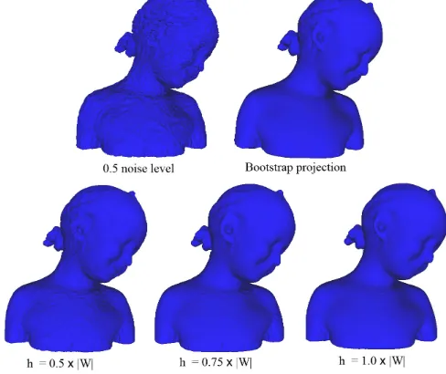
Fig. 1. Bilateral smoothing on the Bimba with 0.5 noise level. Figure shows the noisy model (top left) and its smoothing with naive bootstrap projection (top right). The bottom rows display the bilateral smoothing for severalh2values.|W|is the average value ofWi.
Figure 1 shows Bimba at 0.5 noise level and its naive boot-strap smoothing (top row). Although the bootboot-strap projection on its own has improved the model and made it smoother, the bilateral bootstrap smoothing provides with better results, especially around the feature areas. The results of bilateral smoothing for several h2 values are shown at the bottom
row of the figure. We can see that the choice of h2 affects
the amount of smoothing. In particular, given a value ofh2,
the areas of the model with error values significantly higher thanh2 would not be smoothed. As a rule of thumb, from
Figure 1 bottom row, we can notice that the model is still noisy when the value ofh2 is half the average model error.
Increasing h2 to become 0.75 of the average model error,
or equal to the average model error, gives better smoothing results.
Figure 2 shows a closer comparison between the naive bootstrap projection and bilateral bootstrap smoothing. We can see that the feature areas of the Bimba, such as the ears, hair and the edges at the bottom of the bust, are badly smoothed by naive bootstrap projection, Figure 2 (left). On the other hand, bilateral bootstrap smoothing gives clearly superior results, Figure 2(right).
B. Weights influence on smoothing
The effect of the choice of parameter values forh1andh2
on the smoothing results is shown in Figure 3. In Figure 4, we also display the reflection line renderings of the models to assist us in gauging the smoothness of the model.
Fig. 2. Comparison between naive bootstrap projection (left column) and bilateral bootstrap smoothing with h1 = d and h2 = 0.75|W|(right
[image:3.595.300.546.198.399.2]column).
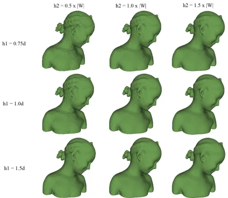
Fig. 3. The result of bilateral smoothing for different values ofh1 and h2.
Fig. 4. Reflection lines for the Bimba model with respect to Figure 3.
influence on a considered point. Thus, when the value of h1 increases, the model generally becomes smoother. This
effect is noticeable in both figures as h1 increases at each
column. We also expect that bilateral smoothing would avoid oversmoothing the feature areas, preserving thus the model features, while, in contrast, a naive filter would smooth out the whole model. As we can see in Figure 3, forh1= 1.5d
the ear of the Bimba starts to deform when the h2 value
increases, that is, the weight of the bootstrap error parameter diminishes. Notice that by increasing h2 to infinity we are
[image:3.595.46.278.293.495.2]left with a single filter based on the distance weight only.
Fig. 5. The result of bilateral smoothing for different values ofh1andh2
on the Bunny.
Fig. 6. Reflection lines for the Bunny model with respect to Figure 5.
We also tested the bilateral smoothing on the Bunny model with 0.5 noise level. The results for various values ofh1and
h2 is shown in Figure 5, while the reflection lines are shown
in Figure 6.
IV. MULTI-PASSBILATERAL SMOOTHING
[image:3.595.304.544.454.651.2] [image:3.595.46.276.552.757.2]procedure is only done once, but the position of each point is updated before we move on to the next one. Thus, if the j-th point is in the neighborhood of the i-th point and the i-th point is processed first, the processing of thej-th point will use the projectedi-th point value instead of the original noisy one. This accelerates the smoothing process making it possible to give reasonable results in one smoothing iteration. A second remark is that the size of neighbourhood,K, is user-defined and fixed for all neighborhoods. In practice, for a model consisting of anything between 10,000 and 50,000 points, choosingK= 100seems to give satisfactory results. However, looking at the results of the previous section, we can also notice that while the Bunny has generally been smoothed nicely, Bimba did not retain several of its features because of oversmoothing. That is, the choice K = 100 caused oversmoothing and a smaller value of K may have been more appropriate, at least at some local neighborhoods of the model. As a third remark, we also notice that the parameters of the bilateral filter h1 andh2 were also fixed.
Algorithm bilateral_multi-pass(K,iteration)
Similar to Algorithm III-A but multiple iterations and adaptively chosen neighborhood size and smoothing parameterh1.
for i=1:N
LetWi=0for alli’s. Find the K-nearest points
zi,j’s for the considered point, j=1:K.
Compute the bootstrap error and obtainWi
end for for i=1:N
Compute neighbourhood sizeKˆi by Equation 4
Compute local average distance between points, dL
Fit the surface polynomial on the neighbourhood
ˆ
Ki and obtain the fitted valueszBi,j.
end for
for k=1:number of iteration for j=1:Kˆi
Project the point and its neighbourhood tozBi,j with weight wi,j such that
zi,j=(1-wi,j)zi,j+wi,jzBi,j as in
Equation 1, but withh1=a∗dL as
defined in Equation 6
end for end for
Algorithm IV: Algorithm for multi-pass bilateral filtering. We propose an improvement of the bilateral filter of the previous section by applying multiple iterations of the smoothing procedure as well as adapting neighbourhood size and spatial distance parameterh1. The procedure is described
in Algorithm IV.
The size of the neighbourhood Kˆi of the i-th point is a
piecewise linear function with two components, given by
ˆ
Ki= max{10, y} (4)
where
y= 10−K
mean(W)Wi+K (5)
see Figure 7. The main idea is that, assuming that the point set contains moderate only noise, a high error indicates
the existence of a model feature in that neighborhood. In this case, we reduce the size of the neighborhood trying to preserve the feature. The lower bound of at least 10 points in each neighborhood ensures that the computations of the local fitting surfaces do not become unstable. Notice that if the error is zero, the size of the neighbourhood should be at its maximum, that is, the user-defined parameter K corresponding to the size of the neighborhood on which we computed the bootstrap error. When the error is equal to the average error over all neighborhoods of the model mean(wi), we have Kˆi = 10. However, mean(wi) could
be replaced by user defined parameter controlling the extent to which we want feature preservation. Notice also, that
ˆ
Ki = 10 is the size of the neighborhood we use for
[image:4.595.369.485.272.380.2]surface fitting while for bootstrap error estimation we always use fixed neighborhood size K. The latter is necessary for obtaining meaningful and comparable error estimates.
Fig. 7. Heuristic selection of neighborhood sizeKˆi.
Finally, the algorithmic parameter h1 is adaptively
com-puted as the product of a user-defined constant a and the average distance between points in the local neighbourhood
ˆ
Ki, denoted dL
h1=a∗dL (6)
Figures 8 and 9 show the Bimba model with 0.5 noise level after being smoothed with the multi-pass bilateral filter. In this example, we chose h1 = 0.1dL andh2 = 0.3|W| and
run 300 iterations. The figures show a significant improve-ment compared to Algorithm III-A. Visually, the area around the hair retained its features and was not oversmoothed as in Algorithm III-A.
Compared to the approach in the previous section, the multi-pass smoothing (Algorithm IV) produces a better result due to mainly three reasons. Firstly, near features, as detected by a high bootstrap error, we project to surfaces that have been fitted to more localized neighborhoods, preserving this way the features better. Secondly we use a localized valuedL
to compute the parameter h1, adapting to the local density
of the model. As the model is not distributed uniformly, the distance from one point to another is not a constant. Thirdly, multiple iterations smooth the model more slowly, preventing the oversmoothing caused by the high values of h1 andh2
that we have to choose if we are applying a single smoothing iteration.
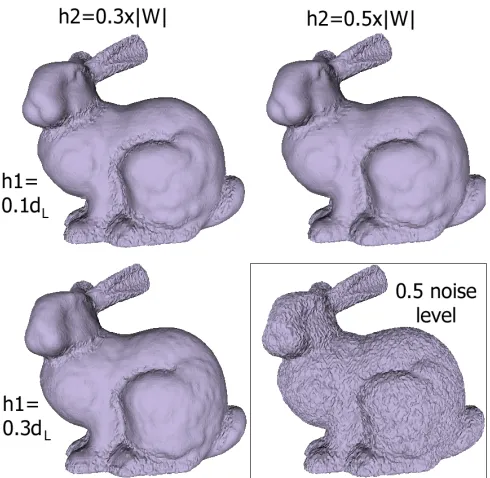
Figure 10 shows the Bunny model at 0.5 noise level after being smoothed by the multi-pass bilateral filter for various values of h1 andh2 and 300 iterations. When the value of
h1 increases, the feature area might be oversmoothed. We
Fig. 8. Multi-pass bilateral smoothing withh1= 0.1dLandh2= 0.3|W|,
[image:5.595.309.546.203.305.2]after 300 iterations.
Fig. 9. Multi-pass bilateral smoothing withh1= 0.1dLandh2= 0.3|W|,
after 300 iterations, original (left) and smoothed (right).
Fig. 10. Multi-pass bilateral smoothing for varioush1 andh2, after 300
iterations. Bottom right figure shows the noisy model before smoothing.
increasing the valuesh2 we can nicely preserve the features.
Indeed, when higher values ofh2 are chosen the features at
the eyes and mouth are preserved, while the area around the leg is also smoother compared to left hand side of the figure. Finally, we compare on Bimba the multi-pass algorithm against two other state-of-the-art smoothing algorithms. Fig-ure 11 shows the result of our method next to Poisson Surface Reconstruction smoothing [11] and AMLS smoothing [12]. We notice that while our method preserves the feature areas better than Poisson, AMLS gives smoother results while still nicely preserving features, as for instance around the ear.
Fig. 11. Comparison with other methods, from left to right: Poisson Surface Reconstruction, our method and AMLS.
V. SUMMARY
In this paper, we used bootstrap error estimates to guide a projection based point set smoothing algorithm. Bilateral filtering was the standard framework employed to incorporate the bootstrap error estimates into the smoothing algorithm. In particular, by using the error estimates as proxies for the quality of the local surface fittings, the proposed smoothing algorithm favours projections on good quality fittings and is able to recover surface characteristics that have been corrupted by noise. The proposed multi-pass variant of the bilateral smoothing was inspired by MLS smoothing, which also is an iterative process projecting points to a fitted surface with certain weights.
While the proposed method has been shown to be able to successfully smooth noisy models with features, several important questions remain unresolved. One of the issues worth researching further is the automatic estimation of the values of the parameters h1 and h2, which at the moment
have to be provided by the user. Another serious current lim-itation is that the method may not always be able to preserve all sharp edges. Notice that this is a common limitation of point set smoothing algorithms based on local neighbourhood processing. The resolution of these limitations can the goal of future research.
REFERENCES
[1] B. Efron, “Bootstrap methods: Another look at the jackknife,” Annals of Statistics, vol. 7, pp. 1–26, 1979.
[2] T. Hastie, R. Tibshirani, and J. Friedman, The Elements of Statistical Learning: Data Mining, Inference, and Prediction. Springer, August 2001.
[3] J. Cabrera and P. Meer, “Unbiased estimation of ellipses by bootstrap-ping,” IEEE Trans. Pattern Anal. Mach. Intell., vol. 18, no. 7, pp. 752–756, 1996.
[image:5.595.85.253.304.414.2] [image:5.595.48.293.494.733.2][5] F. Calakli and G. Taubin, “Ssd: Smooth signed distance surface reconstruction,” Comput. Graph. Forum, vol. 30, no. 7, pp. 1993–2002, 2011.
[6] C. Tomasi and R. Manduchi, “Bilateral filtering for gray and color images,” in Proc. International Conference on Computer Vision. Washington, DC, USA: IEEE, 1998, p. 839.
[7] S. Fleishman, I. Drori, and D. Cohen-Or, “Bilateral mesh denoising,” ACM Trans. Graph., vol. 22, no. 3, pp. 950–953, 2003.
[8] T. R. Jones, F. Durand, and M. Desbrun, “Non-iterative, feature-preserving mesh smoothing,” ACM Trans. Graph., vol. 22, no. 3, pp. 943–949, 2003.
[9] H. Qin, J. Yang, and Y. Zhu, “Nonuniform bilateral filtering for point sets and surface attributes,” The Visual Computer, vol. 24, no. 12, pp. 1067–1074, 2008.
[10] M. Alexa, J. Behr, D. Cohen-Or, S. Fleishman, D. Levin, and C. T. Silva, “Computing and rendering point set surfaces,” IEEE Transac-tions on Visualization and Computer Graphics, vol. 9, no. 1, pp. 3–15, 2003.
[11] M. Kazhdan, M. Bolitho, and H. Hoppe, “Poisson surface reconstruc-tion,” in SGP ’06: Proceedings of the fourth Eurographics symposium on Geometry processing. Aire-la-Ville, Switzerland, Switzerland: Eurographics Association, 2006, pp. 61–70.