Subject specific surgical planning for hip replacement : a novel 2D graphical representation of 3D hip motion and prosthetic impingement information

Subject-Specific Surgical Planning for Hip Replacement: A Novel 2D

Graphical Representation of 3D Hip Motion and Prosthetic Impingement

Information

A

P

,

R

K

,

Y

G

,

J

P

,

D

S

,

and M

A. W

1

WMG, University of Warwick, Coventry CV4 7AL, UK;2Department of Trauma & Orthopaedics, University Hospitals Coventry and Warwickshire NHS Trust, Coventry, UK;3Optimized Ortho, 17 Bridge Street, Pymble, NSW 2073, Australia; and

4

Corin Ltd, Corinium Centre, Cirencester, Gloucestershire GL7 1YJ, UK

(Received 11 November 2018; accepted 29 March 2019)

Associate Editor Joel Stitzel oversaw the review of this article.

Abstract—Prosthetic impingement (PI) following total hip arthroplasty (THA), which arises due to the undesirable relative motion of the implants, results in adverse outcomes. Predicting PI through 3D graphical representation is difficult to compre-hend when all activities are combined for different implant positions. Therefore, the aim of the paper was to translate this 3D information into a 2D graphical representation for improved understanding of the patient’s hip motion. The method used planned implanted geometry, positioned onto native bone anatomy, and activity definitions as inputs to construct the 2D polar plot from 3D hip motion in four steps. Three case studies were performed to highlight its potential use in (a) combining different activities in a single plot, (b) visualising the effect of different cup positions and (c) pelvic tilt on PI. A clinical study with 20 ‘Non-Dislocators’ and 20 ‘Dislocators’ patients after 2 years of THA was performed to validate the method. The results supported the study hypothesis, in that the incidence of PI was always higher in the ‘Dislocators’ compared to the ‘Non-Dislocators’ group. The proposed 2D graphical representation could assist in subject-specific THA planning by visualising the effect of different activities, implant positions, pelvic tilt and related aspects on PI.

Keywords—Total hip replacement, Prosthetic impingement, Implant orientation, Hip joint, Activities of daily living.

INTRODUCTION

Total hip arthroplasty (THA) is a highly effective surgical intervention to relieve pain and restore func-tion to patients with hip osteoarthritis.3,26THA aims to enable the patients to return to their desired

activ-ities of daily living (ADLs) without restrictions and to maximise the life of the implants.22If the biomechan-ical reconstruction is suboptimal, patients are at higher risk of poor function (e.g. limping, ongoing pain), complications (e.g. dislocation), and premature failure of the implants (e.g. implant loosening, excessive wear of the prosthetic joint surfaces). In such circumstances, the patient may have to undergo a revision THA, where the old implants are removed and new ones are inserted. Such revision operations are associated with significant complications (e.g. fractures, bone lossetc.), impose a significant cost burden on the healthcare provider, and are generally less reliable in terms of relieving symptoms and restoring function.18,36 Com-mon reasons for revision surgery are aseptic loosening, wear, and recurrent dislocation.1,7,15,16,20,32,33 In these cases, there is often evidence of prosthetic impinge-ment (PI) as the underlying biomechanical problem.24 PI occurs when the implanted femoral neck comes into contact with the rim of the acetabular cup during ter-minal motion of the hip. This type of contact collision can produce a tilting moment on the cup which may generate shear forces at the bone-implant interface, potentially contributing implant loosening.8,21,33,37 Further motion beyond the impingement point results in the femoral head being levered out of the acetabu-lum, such that it subluxes or dislocates.7,11,15,27 Be-sides, PI can also result in restricted range of movement, and increased pain.2,25It is identified that PI is often the result of surgical misalignment of the femoral and acetabular components during THA.12,17 Therefore, patient-specific surgical planning, that can identify and visualise the effect of component position Address correspondence to Arnab Palit, WMG, University

of Warwick, Coventry CV4 7AL, UK. Electronic mail: [email protected]

on PI, could reduce the chances of impingement, and therefore, improve post-surgical outcomes and min-imise the need for revision surgery.

Historically, surgeons have planned hip replacements in two dimensions (2D), using conventional radio-graphs. Increasingly, however, these procedures are planned in three dimensions (3D) using a pre-operative CT scan. Such 3D plans can then be used for pre-oper-ative analysis of the expected motion of the recon-structed hip, so that potential problems (such as PI) can be anticipated and mitigated by the surgeon. Recently, Schmidet al.23developed a 3D computer-assisted plat-form which provided pre-operative THA planning using medical imaging and optical motion capture. Although the method showed a successful implementation, visu-alisation of different 3D hip motions and graphical representation of their effect on PI were limited. Previ-ous efforts to visualise the dynamic 3D relationship between the components of a THA using 3D graphical representation have proved difficult to compre-hend.2,23,33Therefore, the aim of the paper was to de-velop a method which can translate 3D motion data and PI information into a 2D graphical representation for improved understanding of a patient’s expected hip motion following THA. Furthermore, a clinical study was performed with the following study hypothe-sis—number of patients with observed PI will always be higher in ‘Dislocators’ patients compared to ‘Non-Dis-locators’ patients even for the basic hypothetical hip joint motion, and this could easily be visualised and comprehended through the developed 2D graphical representation. ‘Dislocators’ and ‘Non-Dislocators’ were two patient groups, which were categorised based on the incidences of hip joint dislocation after 2 years of THA. The developed 2D graphical plot from 3D hip joint motion information can potentially be used as a tool to explore the effect of different activities, compo-nent positions, pelvic tilt, and other factors on PI.

The paper is organised as follows. The conceptual novelty of translating 3D hip motion and PI information into a 2D graphical plot is described in the first part of materials and methods followed by its implementation. Thereafter, three case studies and one clinical study were included to highlight the various applications and vali-dation of the method respectively. The rest of the paper describes the results followed by discussion.

MATERIALS AND METHODS

Conceptual Novelty: 2D Graphical Representation of 3D Hip Motion and PI Information

The main novelty of the work is the translation of 3D hip motion and PI information (Fig.1a) into a 2D

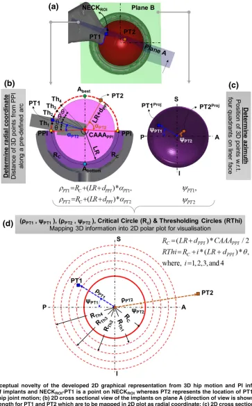
graphical representation though a 2D polar plot (Fig. 1d) without losing any information. This 2D visualisation is intended to provide easier under-standing of the 3D information that is sometimes dif-ficult to comprehend. In this novel method, radial coordinateðqÞrepresents how far the neck area would be from the rim of the liner during an activity (Fig. 1b), whereas azimuth ðwÞ depicts the 3D posi-tions of the neck area into a 2D information (Fig.1c).

Determine the Radial Coordinate

The articulating surface between the femoral head and acetabular implant is located along the curved surface of the acetabular liner, radius of which is the liner radius (LR). The point of prosthetic impingement (PPI) (Fig.1b, yellow dot) is defined as the first contact between the femoral neck and edge of the liner, where the liner face transitions to the rounded edge (fillet in CAD) of the articular margin. Some liners also use a flat chamfer rather than a fillet. Due to fillet or flat chamfer, the PPI is located at a small distance ðdPPIÞ

away from theLR. This distanceðdPPIÞdepends on the

fillet or flat champer at the edge of the articulating surface and on the geometry of the impinging pros-thetic neck. Therefore, instead of considering entire geometry of the neck, only a specific region (NECKROI) which could potentially contact the liner

at PPI is considered for PI analysis. The NECKROIis

defined by a cross-sectional boundary which is gener-ated by cutting the neck geometry with a 3D hypo-thetical hemisphere of radius ðLRþdPPIÞ, and centre

is at liner centre (Fig. 1a). In Fig.1b, the red dotted half-circle (PPI fi Abest fi PPI) represents a 2D

cross section of the 3D hypothetical hemispherical surface, and the NECKROIis the region where the red

dotted curve intersects the neck. Therefore, any point on NECKROIwill always move along the hypothetical

hemisphere surface (Fig. 1a). When NECKROImovies

towards Abestpoint (Fig.1b), the possibility of PI

re-duces, and when it moves towards PPI, it increases. The Cup Articular Arc Angle ðCAAAÞ is most accu-rately measured by the points which are located just below (going from PPI towards Abottomin Fig.1b) the

head. When considering PI, the equivalent angle is measured to the PPI which is located on the face of the liner (Fig.1b), and is therefore marginally larger

ðCAAAþcÞ. The value of c is calculated for the planned implant design. Therefore, the critical arc length (RC) (Fig.1b) from Abottomto PPI is defined by

FIGURE 1. Conceptual novelty of the developed 2D graphical representation from 3D hip motion and PI information. (a) 3D representation of implants and NECKROI-PT1 is a point on NECKROIwhereas PT2 represents the location of PT1 after some time

during a typical hip joint motion; (b) 2D cross sectional view of the implants on plane A (direction of view is shown by black arrow) to show the arc length for PT1 and PT2 which are to be mapped in 2D plot as radial coordinate; (c) 2D cross sectional view on plane B or LF plane (viewing from Abesttowards Abottom) to show the azimuth for PT1 and PT2 which are to be mapped in 2D plot, S:

Superior, I: Inferior, P: Posterior, A: Anterior; (d) Developed 2D polar plot from 3D hip motion information by mapping radial and azimuth of PT1 and PT2, critical and four threshold circles.

Eq. (1) which is the radius of the critical circle of the 2d polar plot (red continuous circle in Fig.1d)

RC¼ ðLRþdPPIÞ CAAAPPI

2

where,CAAAPPI¼CAAAþc

ð1Þ

Suppose, PT1 is one of the points on NECKROI(blue

square in Figs.1a and1b), and PT2, (orange square in Figs.1a and 1b) represents the position of PT1 after some time steps of an activity. PT1 and PT2 makeaPT1

andaPT2angle respectively with the red arrow, defined

by connecting liner centre and PPI. Therefore, the arc length in 3D (Fig.1b), which defines the distance of the NECKROI from the rim of the liner (PPI) along the

hypothetical hemisphere, is mapped to a radial distance in 2D plot (Fig.1d) as defined by Eq. (2).

q_PT1¼RCþ ðLRþdPPIÞ aPT1 q_PT2¼RCþ ðLRþdPPIÞ aPT2

ð2Þ

If during any time steps of an activity,aPT1oraPT2

becomes zero (0) or negative,qPT1orqPT2will be equal

or less than RC respectively. This represents the

situ-ation of a PI which could easily be identified using the polar plot as part of NECKROIwill be either touching

or inside the critical red circle.

In order to provide a better visualisation of the relative distance of the NECKROI with respect to red

critical circle in 2D polar plot, additional thresholding circles are included (red dotted circles in Fig.1d). Four thresholding positions (Th1, Th2, Th3, and Th4) are defined on the 3D hypothetical hemisphere (Fig.1b). When the NECKROI moves towards point Th1, Th2,

Th3, and Th4 along the red circle of radius

ðLRþdPPIÞ, the distance from the NECKROI to the

rim of the liner increases, and therefore, the propensity of PI reduces, and vice versa. These thresholding points are separated with each other by an user defined angle h (Fig. 1b) with an arc length ðLRþdPPIÞ h.

Also, the first thresholding point (Th1) and PPI is also separated by same angleh. Therefore, the radius of the thresholding circles, which are related to thresholding points, are as follows

RThi¼RCþi ðLRþdPPIÞ h;

wherei¼1; 2;3;and 4 ð3Þ

The criteria of choosing thresholding points, and subsequently, thresholding circles depends on the value of anglehwhich is entirely user defined. In this work, the anglehis defined by some user-specific percentage of CAAA to make the thesholding points specific to implant design. However, value of angle h could be chosen as a fixed value which would not depend on CAAA.

Determine the Azimuth

The polar plot can be thought to be drawn on the plane of the liner face (LF) (plane B in Fig.1a) which are divided into four anatomic quadrants (Fig. 1c) i.e. anterior–superior (S–A), posterior–superior (P–S), anterior–inferior (A–I), and posterior–inferior (P–I). These quadrants are created by constructing two per-pendicular axes: Superior-Inferior and Posterior-An-terior which pass through the liner centre. The points of the NECKROI, moving along the hypothetical 3D

hemisphere surface, could be projected on the LF plane (Fig. 1c). Suppose, PT1 and PT2 are projected on LF plane to get the projected points PT1Proj and PT2Proj (Fig. 1c). These projected points create an angle wPT1and wPT2respectively with respect to

Pos-terior-Anterior axis. These angles (wPT1 and wPT2)

could then be used as the azimuth of the 2D polar plot (Fig. 1d).

Implementation of the Method

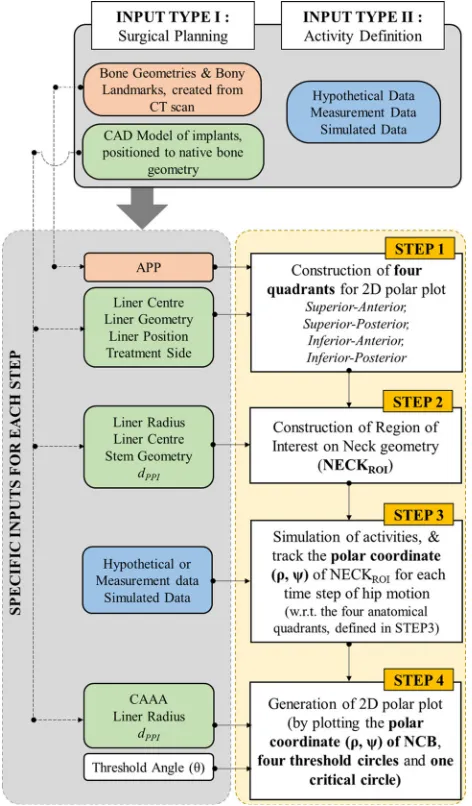
The following sections describe all the inputs and steps required for the method to translate 3D hip motion into a 2D graphical representation (Fig. 2).

Inputs

There were two types of input required for the method—(A) Input Type I and (B) Input Type II (Fig. 2). (A) Input Type I was associated with 3D surgical plan, and dealt with the following main as-pects: (a) CT scanning, (b) construction of bone geometries, (c) identification of bony landmarks, (d) CAD model of planned implants, and (e) planned implant positioning. Finally, bony landmarks and the implant geometries, positioned onto the native bone geometry according to the surgical plan, were used as Input Type I. (B) Input Type II represented the hip motion under consideration. This hip motion could be hypothetical activity (e.g. simple flexion, extension

etc.), measured activity (e.g. using gait analysis), or simulated activity (e.g. generated using other software such as multi-body dynamics software).

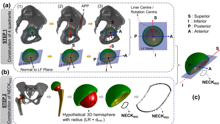
Step 1: Construction of Four Quadrants

geometry according to the surgical plan, and (d) treatment side (hip joint side). Firstly, a parallel plane of the APP was constructed which intersected the LF plane at liner centre (Fig.3a (2)). The intersected line vector was the superior-inferior (SI) axis of the polar plot (Fig.3a (2)). It divided the LF plane equally into two parts—posterior and anterior. Finally, posterior-anterior (PA) axis was defined by a line on LF plane, which was perpendicular to SI axis and passed through liner centre (Fig.3a (3)).

Step 2: Construction of NECKROI

Only a specific region (NECKROI), which would

come first in contact with liner at PPI, was considered for PI analysis. The rest of the neck geometry was therefore ignored. Four inputs were required for this step

(Fig. 2)—liner radius, liner centre, actual neck geome-try, anddPPI. The NECKROIwas then constructed by

intersecting the neck/stem geometry with a hypothetical 3D hemisphere (Figs. 1a and3b) of radiusðLRþdPPIÞ

and centre at liner centre. This procedure was performed using Matlab function ‘fastMesh2Mesh’29 which em-ployed Ray-Triangle intersection algorithm13 to auto-matically calculate the intersection points between two STL geometries with triangular mesh. It used triangular face ids and vertices of the hypothetical sphere and ac-tual neck as inputs, and calculated a set of intersection points which was actually used as NECKROI(Fig.3b).

No assumption was made regarding the geometric pro-file of the neck. Therefore, this method would work for any neck geometry as the shape of the NECKROIwill

depict the true neck profile at a ðLRþdPPIÞdistance

from liner centre. Figure3c shows the 3D position of NECKROIwith respect to four quadrants defined on LF

plane during a particular time step of an activity.

Step 3: Simulation of Activities to Get Polar Coordinate (q,w) of the NECKROIfor Each Time Step

Input Type II (Fig.2) was required to get the move-ment of NECKROI. The radial coordinate ð Þq was

identified for each point on NECKROI using the

fol-lowing steps. (I) A vectorðvPLÞwas constructed using

liner centreðL0Þand a point on NECKROIðPROIÞfor a

time step of the activity. The length of the vector (vPL)

was ðLRþdPPIÞas all the points on NECKROIwere

located atðLRþ dPPIÞdistance from liner centreðL0Þ. (II) The angle ð Þa between the vector vPL and the LF

plane signified that the pointPROIwasaangle away from

the LF plane. The liner is not a full hemisphere as the

CAAAPPIis less than 180. Therefore, the angle between

LF plane and the axis (or plane), which was used to measuredCAAAPPI(line/plane connecting liner centre

and PPI (s), see Fig.1b), is

n¼ðpCAAAPPIÞ

2 ð4Þ

Therefore, the point PROI was effectively make an

angleða þ nÞwith the line (or plane) connecting liner centre and PPI. (III) the arc length LPROI

arc

was then calculated as,

LPROI

acr ¼ ðLRþ dPPIÞ ðaþnÞ ð5Þ

It represented that the point PROI was LParcROI arc

distance away from PPI. (IV) Finally,LPROI

arc was added

to radiusRCto get q

q¼RCþLParcROI ð6Þ

If there is any impingement,LPROI

arc would be negative

andq would be less thanRC.

FIGURE 2. A brief overview of the method along with the inputs and steps involved to generate 2D polar plot form 3D hip motion and PI information for ADLs.

The azimuth of the same pointðPROIÞwas identified

using following steps. The projectionðPvÞof the vector vPLon the LF plane was calculated, and thereafter, the

angle (w1) betweenPvand PA axis was measured. If the

pointðPROIÞwas located in quadrant Superior-Posterior

or Superior-Anterior, the azimuthð Þw would be same as the calculated w₁. If the pointðPROIÞwas situated on

quadrant Inferior-Posterior or Inferior-Anterior, the azimuthð Þw would be 2ð pw₁Þ. Using this method, the polar coordinatesðq;wÞof all the points on NECKROI

were calculated for each time steps (Fig.2).

Step 4: Generation of 2D Polar Plot

Finally, the polar coordinatesðq;wÞfor all the points on NECKROI for each time step of an activity were

plotted on the 2D polar plot along with the critical and four thresholding circles using four inputs—CAAAPPI,

liner radius, user defined thresholding angle ðhÞ, and

dPPI (Fig.2). In this work, h is defined as 5% of CAAAPPIfor a suitable visualisation of the thresholding

circles although any values ofhcould be chosen as it is entirely user defined. Ifhis very small, the thresholding circles would be very close together and it would look too cramped. On the other hand, large values ofhwould locate the thresholding circles farther apart which would affect the visualisation.

CASE STUDIES

The 3D plans for a right THA were used to demonstrate the useful features of the 2D graphical representation in designing patient-specific THA

planning. Three cases were considered: (a) Case I: The effect of moving the hip joint into different functional positions for a particular implant position; (b) Case II: The effect of changing acetabular cup orientation on PI; and (c) Case III: The effect of simulated pelvic tilt on PI for a particular implant position. Input Type I for the method (Fig. 2) was provided by experienced engineers at Corin Ltd, who provide a 3D THR planning service for surgeons. This retrospective analysis of the data from Corin was approved by Bellberry Human Research Ethics Committee (BHREC) - study number 2012-03-710. The position of acetabular components was defined by radiographic inclination and anteversion angle, as defined by Mur-ray,14 and represented as inc/ant (e.g. 33/25) in this paper.

Case I (Table1) was considered because it reflects the way in which surgeons assess the function of the THA during the surgery. After inserting the THA implants, it is normal practice for the surgeon to move the hip into relatively extreme functional positions to check that the hip is not prone to PI or dislocation. These positions typically include deep hip flexion with internal rotation and full extension with external rotation.5Based on this common practice, four hypo-thetical hip movements were defined (Input Type II) for the Case I, and subsequently, the 3D hip motion and PI information for all these activities (Table 1) were included into the 2D polar plot.

(Table1) were simulated for each orientation. Polar plots were then generated to highlight the effect of changing acetabular orientation on predicted PI for these four activities.

Case III was of interest because the pelvis is known to significantly flex (anterior tilt) and extend (posterior tilt) during ADLs, and therefore, an important factor during hip joint movement analysis. Three scenarios were considered: (a) no pelvic tilt, (b) posterior, and (c) anterior pelvic tilt19 (Table3) for a given femur movement. It was assumed that pelvic tilt occurred maximally during flexion activity, and therefore, only the hip flexion and IRFlex(Table 1) were analysed.

Typical representative cup positions within the safe zone10 were considered for case II and III to illustrate graphically the effect of different cup positions and pelvic tilt on PI respectively.

Clinical Study and Validation of the Method

In order to validate the method, the data of patients who had previously undergone a THA was analysed. The anonymised data was provided by Corin Ltd, which was approved by BHREC (2012-03-710). Two groups of patients were studied, based on the outcome of their THA after 2 years: (a) ‘Non-Dislocators’ where there had been no postoperative episodes of hip dislocation; (b) ‘Dislocators’ where there had been at least one clinical episode of dislocation of the THA. Table3 summarises the patient characteristics and intraoperative data used for this study. 3D models of the implants, positioned onto the native bone geome-tries, and bony landmarks were used as Input Type I which were extracted from post-operative CT scan by dedicated experienced engineers in Corin Ltd.

For Input Type II, two scenarios were considered as subject-specific hip motion data was unavailable for this study. In Scenario I, four hypothetical activities (Table1) which are generally performed during sur-gery, were used. Three sets of extreme position of IRFlex and ERExt were used in this study (Table4)

based on the values by Tannast et al.,28 whereas the final positions of flexion and extension were kept same (Table4). In Scenario II, four pure joint motions at supine position were considered (Table4). The ex-treme position of each activity was obtained from the reference value of Turleyet al.31,33

It is well known that a significant proportion of THA dislocations occur due to PI.7,11,15,24 Therefore, the hypothesis of the study was that the number of patients with observed PI will be always higher in ‘Dislocators’ patients compared to ‘Non-Dislocators’ group even for the basic hypothetical activities con-sidered through Scenario I and II with generalised range of motion (Table4).

RESULTS

The results of three case studies are briefly descried below to highlight the various aspects of the 2D pre-sentation of the 3D hip motion and PI information.

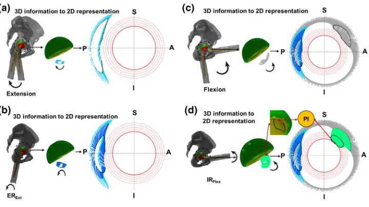
Case Study I: Inclusion of Different Activities in a Same 2D Plot

Case study I displayed how 3D NECKROI

move-ment during different activities could be combined in a single 2D polar plot (Fig.4). 3D motion of NECKROI

during extension activity was translated into 2D polar plot (Fig.4a). It was observed that the chances of PI during extension activity was minimal as the NECKROI didn’t even cross the outermost threshold

circle, and all of extension movement was confined around the posterior region of the liner (Fig.4a). Similarly, the 3D NECKROI movement for both

extension and ERExt were combined into 2D plot

(Fig. 4b). It showed that the final position of ERExt

crossed the outer most 4th threshold circle, and almost touched the 3rd threshold circle in the posterior region of the liner/cup, suggesting minimal propensity of PI (Fig. 4b). Similarly, it was observed that flexion of 90 had minimal possibility of PI as NECKROIonly

tou-ched the third threshold circle in superior-anterior quadrant (Fig.4c). However, the final position of the IRFlexcrossed the critical red circle in superior-anterior

quadrant (Fig. 4d). This indicated that there was a high chance of PI due to 40of IRFlex. The actual 3D

impingement was shown using cup/liner geometry and NECKROIwhere it touched rim of the liner (Fig. 4d).

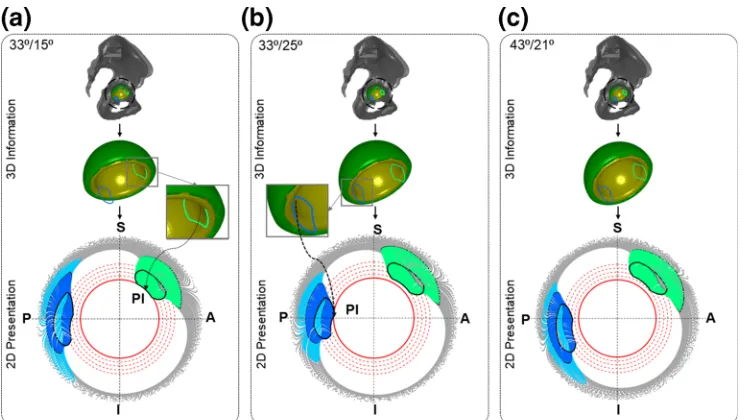
Case Study II: Effect of Cup Orientation

Case Study II showed how 2D polar plot can be used to highlight the effect of cup position on PI for same hip movement. It was observed that there was a chance of PI during IRFlexat superior-anterior region

of the liner when the acetabular cup was positioned with 33inclination and 15anteversion (Fig.5a). The propensity of PI in ERExt was minimal as NECKROI

only crossed 3rd threshold circle (Fig.5a). On the other hand, there was a much higher possibility of PI in superior-posterior region during the ERExt when

cup position changed to 33 inclination and 25 anteversion (Fig.5b). However, the potential for anterior impingement during IRFlexwas now reduced

as NECKROIwas 1st threshold circle away. When cup

position was changed to 43 inclination and 21 anteversion, the overall chances of PI was reduced, as the NECKROIwas at least one threshold circle away

from the acetabular margin for all simulated activities (Fig. 5c).

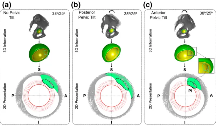
Case Study III: Effect of Pelvic Tilt Orientation

Case Study III depicted how 2D polar plot can be used to highlight the effect of pelvic tilt on PI propensity when performing the same pre-defined activities for a particular cup position (Fig.6). NECKROI crosses 2nd threshold circles during last

time step of IRFlexwhen no-pelvic tilt was considered

(Fig.6a). If the subject had posterior pelvic tilt during flexion, it would further reduce the chance of PI, as NECKROImoved away from 1st to 3rd threshold circle

(Fig.6b). In contrast, anterior pelvic tilt clearly increased the possibility of PI, as the NECKROI

tou-ched the critical circle (Fig.6c).

Clinical Study and Validation of the Model

It was observed that the number of patients with PI was indeed always higher in the ‘Dislocators’ group

compared to the ‘Non-Dislocators’ group (Fig. 7), which was consistent with the study hypothesis. For Set 1 in Scenario I, there was no detection (Fig.7) as the ROM considered for ERExtand IRFlex might not

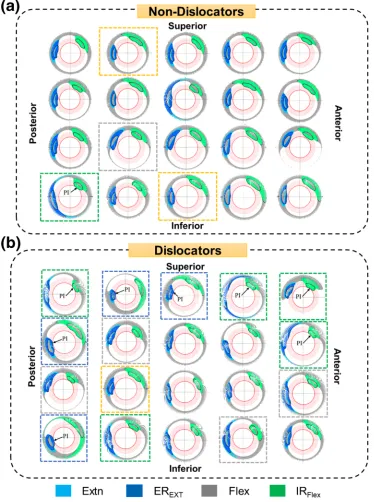
be extreme enough to cause any PI. When the ROM for these two activities increased, the number of detection was increased for both Set 2 and Set 3. However, the number of detections in ‘Dislocator’ was always higher-9 ‘Dislocators’ vs. 1 ‘Non-Dislocators’ in Set 2 and 14 ‘Dislocators’ vs. 4 ‘Non-Dislocators’ in Set 3. Scenario II depicted the similar results i.e. 12 ‘Dislocators’ patients with PI compared to 2 patients in ‘Non-Dislocators’ group. In Set 2, PI occurred due to IRFlex and ERExt in 5 and 4 cases respectively

(Fig. 8b), resulted in total 9 for ‘Dislocators’ group whereas IRFlex caused only 1 case of PI in

‘Non-Dis-locators’ (Fig.8a). In Set 2, it was also observed that 4 and 1 patients in ‘Dislocators’ group had high chance TABLE 1. Definition of the hypothetical hip movements used for Case I.

Activities Initial position Final position

Extension (Extn) Supine 10Extension

External rotation at extension (ERExt) 10Extn, 0ERExt 20ERExt

Flexion (Flex) Supine 90Flexion

Internal rotation at flexion (IRFlex) 90Flex, 0IRFlex 35IRFlex

These hypothetical activities are generally performed by surgeon during THA.

TABLE 2. Description of Case II and Case III to highlight the effect of cup position and pelvic tilt respectively on PI through 2D polar plot.

Case II Case III

Cup position (inc/

ant) Activities

Pelvic tilt

2D Plot

pro-duced Pelvic tilt Activities

Cup position (inc/ ant)

2D plot pro-duced

33/15 All four No One No pelvic tilt Flex & IR 38/25 One

33/25 All four No One Posterior pelvic tilt

5

Flex & IR 38/25 One

43/21 All four No One Anterior pelvic tilt 5 Flex & IR 38/25 One

*inc/ant = radiographic inclination and anteversion angle, as defined in Murray14_.

TABLE 3. Patient characteristics and intraoperative data.

Characteristic Non-Dislocators (n= 20) Dislocators (n= 20)

Sex (male/female) 13/7 9/11

Age (years) 65.1±9.5 64.1±8.43

Treatment side (left/right) 10/10 12/8

Cup size (diameter in mm) 53 (50–60) 51.8 (46–56)

Head size (diameter in mm) 34.2 (32–36) 34.6 (28–40)

Cup inclination () 40.3±4.6 41.2±8.1

Cup anteversion () 22.2±6.9 25.1±8.5

Stem anteversion () 10.4±10.3 17.6±7.6

dPPI 1.1±0.89 1.4±1.1

of PI if the extreme position of IRFlexand ERExtwould

increase respectively (Fig.8b). This was evident from the results of Set 3 where final position of IRFlex and

ERExt were increased (Table4). Similar observation

was obtained when ‘Non-Dislocators’ group was con-sidered. The patients with higher PI possibility (2 and 1 for IRFlexand ERExtrespectively) from Set 2 in

‘Non-Dislocators’ group (Fig.8a) had PI when final posi-tions of IRFlex and ERExt were increased in Set 3

(Table4).

DISCUSSION

This paper introduces a novel 2D graphical repre-sentation of 3D hip motion and PI information, which are difficult to visualise and comprehend. The pro-posed method has several features which could be modified according to the user’s requirements. Firstly, there were four threshold circles which were used to intuitively visualise the relative distance of the NECKROI from critical circle. Besides, the extreme

TABLE 4. A summary of the definition of activities (Input Type II) used for Scenario I and II for the validation of the method through clinical study.

Activities Initial position Final position

SCENARIO I: pure joint & combined hip motions

SET1 Extension (Extn) Supine 10Extn

Flexion (Flex) Supine 90Flex

External rotation at extension (ERExt) 10Extn, 0ERExt 20ERExt

Internal rotation at flexion (IRFlex) 90Flex, 0IRFlex 25IRFlex

SET2 Extension (Extn) Supine 10Extn

Flexion (Flex) Supine 90Flex

External rotation at extension (ERExt) 10Extn, 0ERExt 25ERExt

Internal rotation at flexion (IRFlex) 90Flex, 0IRFlex 35IRFlex

SET3 Extension (Extn) Supine 10Extn

Flexion (Flex) Supine 90Flex

External rotation at extension (ERExt) 10Extn, 0ERExt 30ERExt

Internal rotation at flexion (IRFlex) 90Flex, 0IRFlex 45IRFlex

SCENARIO II: pure joint hip motion

Extension (Extn) Supine 10Extn

Flexion (Flex) Supine 90Flex

External rotation (ER) Supine, 0ER 45ER

Internal rotation (IR) Supine, 0IR 45IR

FIGURE 4. Results from ‘Case study I’ to show how a single 2D polar plot can be used to combine all the 3D information, generated from different activities. S, I, P, and A represent Superior, Inferior, Posterior, and Anterior respectively. (a), (b), (c) and (d) show the mapping of 3D NECKROImovement during extension (sky blue), EXExt(blue), flexion (grey), and IRFlex(green) respectively

into a 2D polar plot. The black NECKROIrepresents last time step of each activity.

position during any hip joint motion is subject-specific and varies considerably amongst patients. Therefore, when generalised extreme positions of an activity is used based on previous study, it was either over or under estimated for that particular patient. However, using threshold circles, it could be visually compre-hended how much over or under estimation would affect PI (Fig.8). Therefore, it entirely depends on the user whether to keep thresholding circles at all or how many thresholding circles should be used or what would be the radial separation distance between the thresholding circles. Secondly, non-linear scaling in radial direction of the 2D plot could be used to high-light further the positional differences of NECKROIfor

different scenarios. However, it should be noticed that the radius of the critical and four thresholding circles should also be changed using same non-linear scaling for consistency. In addition, type of non-linearity is also very crucial. Non-linearity functions such as exponential function which is monotonically strictly increases or decreases would be best. Thirdly, colour codes to represent critical and threshold circles, and locus of NECKROIfor different activities are entirely

user specific. Finally, it was never claimed that the values used in the paper for extreme positions of hip joint motion, cup positions or pelvic tilt were measured subject-specifically. These were typical representative values within their ranges as identified from the liter-ature. These values were used just to illustrate various features of the proposed 2D plot, and therefore, the proposed method is not restricted to these values only.

Therefore, the developed 2D plot could be a valuable tool to assist surgeons in the surgical planning of THA by analysing the effect of different ADLs, cup posi-tions, pelvic tilt and other aspects on PI.

Inclusion of Several Activities in a Single 2D Plot

One of the main advantages of the plot was that it could combine all of the 3D hip motion and PI information, generated during different activities, in a single 2D polar plot. As a result, it was easy to visualise which activity, and specifically, what range of move-ment of the activity, could cause PI. Recently, Hsu

et al.6 developed a visualisation method based on similar concept i.e. mapping the movement of femoral neck with respect to the cup from a 3D sphere onto a 2D plane. However, Hsu et al.6 method tracked the movement of neck axis end point only whereas the proposed method considered the true shape of the actual neck geometry through NECKROI. Therefore,

effect of different stem geometries on PI, which might be difficult to highlight using Hsu et al.6method, can still be visualised using the proposed method of the paper. Four hypothetical activities, which are quite commonly assessed by the surgeons during THA,5 were used in the case study to just demonstrate a useful feature of the plot. It was not claimed that the activities were subject specific, nor accurately measured. How-ever, the extreme positions of the simulated activities were well within the ranges described in the litera-ture.9,28,30,31 Different activities to those presented in

FIGURE 5. Results from Case Study II to show the effect of cup position on PI. (a), (b) and (c) show the 2D representation of 3D NECKROImovement during extension (sky blue), ERExt(blue), flexion (grey), and IRFlex(green) activities for different cup positions

at 33°/15°, 33°/25°, and 43°/25°respectively where first and second angles are inclination and anteversion respectively. S, I, P, and A represent Superior, Inferior, Posterior, and Anterior respectively. The black NECKROIin 2D polar plot represents last time step of

the paper could also be visualised using different col-ours (Fig.4). Also, the possibility of PI (if not explic-itly observed) was recognised easily by comparing the position of NECKROIwith respect to threshold circles.

In addition, the location of impingement was presented in terms of anatomic quadrants i.e. anterior–superior, posterior–superior, anterior–inferior, and posterior– inferior. This information is likely to result in a more comprehensive assessment of the hip joint movement.

Visualise the Effect of Cup Position on PI

The effect of cup position for a given set of activities could easily be visualised using the 2D polar plot (Fig.5). It was observed that some cup positions cre-ated PI where other positions did not for a given femur

movement (Fig. 5). In this study, three particular cup positions were analysed, but any combination of inclination/anteversion angles could be fed into the model to explore their effects on PI. Therefore, this plot can be used to intuitively suggest a better cup position for the patient provided they are compatible with other selection criteria. Cup positions, combined anteversion or implant geometries are associated with surgical plan, and therefore, these aspects are the part of ‘Input Type I’. As a result, the effect of these factors on PI could easily be visualised without any change in the steps (Step 1 to Step 4 in Fig.2) of the proposed method.

Visualise the Effect of Pelvic Tilt on PI

Pelvic rotations have a direct effect on the functional orientation of the cup/liner,19 and subsequently, on PI. Using Case III, it was demonstrated that the pro-posed 2D plots could visualise the effect of pelvic tilt orientation (posterior or anterior) on PI for a given femur movement and cup positions (Fig. 6). These orientations and the amount of pelvic tilt are subject-specific and also depend on type of activities. There-fore, some hypothetical but clinically relevant values of pelvis tilt19 were used for a given hypothetical femur movements as the objective of the Case III was only to highlight the capability of 2D plot in visualising the effect of pelvic tilt on PI. However, effect of any activity-specific pelvic tilt on PI for any subject can easily be visualised using the proposed 2D plot. FIGURE 6. Results from Case Study III to show the effect of pelvic tilt on PI. (a), (b) and (c) show the 2D representation of 3D NECKROImovement during flexion (grey), and IRFlex(green) activities when no-pelvic tilt, posterior and anetrior pelvic tilt are

considered respectively for a particular cup position. S, I, P, and A represent Superior, Inferior, Posterior, and Anterior respectively. The black NECKROIin 2D polar plot represents last time step of each activity. The grey and green NECKROIin 3D

geometry show the last time step of flexion and RFlexrespectively.

FIGURE 7. Results from clinical study which is used for validation of the method. Number of patients with observed PI is always higher for ‘Dislocators’ group compared to ‘Non-Dislocators’ group for each of the scenario.

Clinical Study and Validation of the Method

In this paper, the clinical study was used as a validation procedure of the proposed method rather than finding any clinical significance. For different scenarios, the proposed method always identified more patient with observed PI in ‘Dislocators’ group compared to ‘Non-Dislocators’ group, which

corresponded to study hypothesis. It can therefore be inferred that the implementation of the proposed method was correct. In addition, the clinical study revealed that the method can easily be used for any implant geometries and their positions (cup incli-nation/anteversion or combined anteversion etc.) as highlighted in Table1.

FIGURE 8. 2D Graphical representation of the 3D hip motion considered in ‘Set 2’ of ‘Scenario-I’ for each (a) ‘Non-Dislocators’ and (b) ‘Dislocators’ patient. Each 3D hip motion is colour coded in 2D plot, and extreme position of each hip motion is highlighted with black colour. The green and blue dotted box show that the PI occur due to IRFlexand ERExtrespectively. The yellow and grey

box show that those patient have high chance of PI due to ERExtand IRFlexrespectively if the extreme positions of these activities

One of the advantages of this 2D graphical repre-sentation was that the surgeons could predict which activity might cause PI if the extreme position of the activity would increase a little (Fig.8). For a particular activity, there might not be any observed PI in the 2D plot. However, the location of NECKROIwith respect

to the thresholding circles could convey the possibility of potential PI if the extreme position of the activity would increase. There is a strong trend to use 3D-data in routine clinical practice especially in Orthopedics. Availability of 3D-CT data might eventually help to represent PI analysis through digital display of 3D model which might reflect the actual realistic scenarios. However, according to the authors’ opinion, it would be difficult to visualise and comprehend the actual distance between the rim of the liner and the neck from the digital display of 3D model as this distance is not a linear distance, rather it is a nonlinear arc distance. It could be observed from Fig.4that the actual distance of the NECKROI from the rim of the cup was not

comprehended well from the 3D representation al-though when this curvilinear distance was mapped to a linear distance in a 2D plot, it was easily compre-hended and comparable. Another advantage of this 2D plot is that it is easier to understand in printing and book format compared to the 3D model. During pri-mary and revision surgery, the surgeon has to decide whether to change the orientation of the acetabular component, the femoral component, or both. There is currently limited functional information available to the surgeon planning primary and revision surgery that can inform the specific changes to the THA that are necessary, and therefore, this method has the potential to aid pre-operative surgical decision making in these challenging surgical cases.

LIMITATIONS

Firstly, the hypothetical activities and the pelvic tilt, used in the case studies, were defined based on the generalised range of motion data from the literature as subject-specific data was not available. If accurate di-rect measurement was available, this could easily be fed into the model to generate more accurate results. Secondly, there was no direct validation of the method. It is not possible at present to accurately directly re-cord pelvic tilt, femoral movements, and the presence of impingement simultaneously in real-time in patients. Our indirect validation, performed through the clinical study, produced results which are consistent with clinical experience. Thirdly, the effects of changing the design of the femoral component or combined ante(version) on PI were not explicitly analysed in this paper, but the method would readily permit this as this

information is only related to Input Type I. Finally, it must be acknowledged that there are other biome-chanical issues such as bone impingement4 that can compromise the function and longevity of the THA which this method does not consider.

FINAL REMARKS

This paper introduces a novel concept of translating 3D hip motion and PI information into a 2D graphical representation through a 2D polar plot. 3D hip motion information of several activities could be combined into this single 2D plot to identify the activities which are prone to cause PI, and the anatomic region of the cup where this impingement would occur. In addition, this 2D plot is easier to comprehend, and therefore, could potentially be used as a tool for exploring the effect of different cup positions, pelvic tilt, combined anteversion and many other aspects of the surgical procedure on PI propensity to inform patient-specific primary and revision THA planning.

ACKNOWLEDGEMENTS

The study was funded by Corin Ltd.

OPEN ACCESS

This article is distributed under the terms of the Creative Commons Attribution 4.0 International License (http://creativecommons.org/licenses/by/4.0/), which permits unrestricted use, distribution, and repro-duction in any medium, provided you give appropriate credit to the original author(s) and the source, provide a link to the Creative Commons license, and indicate if changes were made.

REFERENCES

1

AOA. Australian Orthopaedic Association National Joint Replacement Registry (AOANJRR), Hip, Knee & Shoul-der Arthroplasty: 2017 Annual Report. Adelaide: AOA, 2017.

2

Brown, T. D., and J. J. Callaghan. Impingement in total hip replacement: mechanisms and consequences. Curr. Orthop.22:376–391, 2008.

3

Enocson, A., C. J. Hedbeck, J. Tidermark, H. Pettersson, S. Ponzer, and L. J. Lapidus. Dislocation of total hip replacement in patients with fractures of the femoral neck.

Acta Orthop.80:184–189, 2009.

4_{Harkess, J. W., and J. R. Crockarell. In: Campbell’s}

Operative Orthopaedics13th, edited by F. M. Azar, J. H.

Beaty, and S. T. Canale. Amsterdam: Elsevier, 2017, pp. 165–321.

5

Harkess, J. W., and J. R. Crockarell. Part II: Chapter 3 Arthroplasty of the hip. In: Campbell’s Operative Ortho-paedics, 4-Volume Set13th, edited by F. M. Azar, S. T. Canale, and J. H. Beaty. Amsterdam: Elsevier, 2017, pp. 165–321.

6

Hsu, J., M. de la Fuente, and K. Radermacher. Calculation of impingement-free combined cup and stem alignments based on the patient-specific pelvic tilt.J. Biomech.82:193– 203, 2019.

7_{Kluess, D., H. Martin, W. Mittelmeier, K. P. Schmitz, and}

R. Bader. Influence of femoral head size on impingement, dislocation and stress distribution in total hip replacement.

Med. Eng. Phys.29:465–471, 2007.

8

Ko, B. H., and Y. S. Yoon. Optimal orientation of im-planted components in total hip arthroplasty with poly-ethylene on metal articulation.Clin. Biomech.23:996–1003, 2008.

9

Kubiak-Langer, M., M. Tannast, S. B. Murphy, K. A. Siebenrock, and F. Langlotz. Range of motion in anterior femoroacetabular impingement. Clin. Orthop. Relat. Res.

458:117–124, 2007.

10

Lewinnek, G. E., J. L. Lewis, R. Tarr, C. L. Compere, and J. R. Zimmerman. Dislocations after total hip-replacement arthroplasties.J. Bone Joint Surg. Am.60:217–220, 1978.

11

Malik, A., A. Maheshwari, and L. D. Dorr. Impingement with total hip replacement.J. Bone Joint Surg. Am.89:339– 346, 2007.

12_{Mellon, S. J., G. Grammatopoulos, M. S. Andersen, H. G.}

Pandit, H. S. Gill, and D. W. Murray. Optimal acetabular component orientation estimated using edge-loading and impingement risk in patients with metal-on-metal hip resurfacing arthroplasty.J. Biomech.48:318–323, 2015.

13

Mo¨ller, T., and B. Trumbore. Fast, minimum storage ray-triangle intersection.J. Graph. Tools2:21–28, 1997.

14

Murray, D. W. The definition and measurement of acetabular orientation.J. Bone Joint Surg. Br.75:228–232, 1993.

15

Nadzadi, M. E., D. R. Pedersen, H. J. Yack, J. J. Cal-laghan, and T. D. Brown. Kinematics, kinetics, and finite element analysis of commonplace maneuvers at risk for total hip dislocation.J. Biomech.36:577–591, 2003.

16

NJR. 14th Annual Report of the National Joint Registry of England, Wales, Northern Ireland and the Isle of Man. 2017.

17_{Palit, A., M. A. Williams, G. A. Turley, T. Renkawitz, and}

M. Weber. Femur First navigation can reduce impingement severity compared to traditional free hand total hip arthroplasty.Sci. Rep.7:7238, 2017.

18_{Patel, A., G. Pavlou, R. E. Mu´jica-Mota, and A. D. Toms.}

The epidemiology of revision total knee and hip arthro-plasty in England and Wales. A comparative analysis with projections for the United States. A study using the Na-tional Joint Registry dataset. Bone Joint J. 97(8):1076– 1081, 2015.

19

Pierrepont, J., G. Hawdon, B. P. Miles, B. O. Connor, J. Bare, L. R. Walter, E. Marel, M. Solomon, S. McMahon, and A. J. Shimmin. Variation in functional pelvic tilt in patients undergoing total hip arthroplasty. Bone Joint J.

99(8):184–191, 2017.

20

Renkawitz, T., M. Haimerl, L. Dohmen, S. Gneiting, M. Wegner, N. Ehret, C. Buchele, M. Schubert, P. Lechler, M. Woerner, E. Sendtner, T. Schuster, K. Ulm, R. Springorum, and J. Grifka. Minimally invasive computer-navigated total hip arthroplasty, following the concept of femur first

and combined anteversion: design of a blinded randomized controlled trial.BMC Musculoskelet. Disord.12:192, 2011.

21

Sakai, T., N. Sugano, T. Nishii, K. Haraguchi, T. Ochi, and K. Ohzono. Optimizing femoral anteversion and offset after total hip arthroplasty, using a modular femoral neck system: an experimental study. J. Orthop. Sci. 5:489–494, 2000.

22

Sakai, T., N. Sugano, K. Ohzono, T. Nishii, K. Haraguchi, and H. Yoshikawa. Femoral anteversion, femoral offset, and abductor lever arm after total hip arthroplasty using a modular femoral neck system.J. Orthop. Sci.7:62–67, 2002.

23_{Schmid, J., C. Cheˆnes, S. Chague´, P. Hoffmeyer, P.}

Christofilopoulos, M. Bernardoni, and C. Charbonnier. MyHip: supporting planning and surgical guidance for a better total hip arthroplasty.Int. J. Comput. Assist. Radiol. Surg.10:1547–1556, 2015.

24

Scifert, C. F., P. C. Noble, T. D. Brown, R. L. Bartz, N. Kadakia, N. Sugano, R. C. Johnston, D. R. Pedersen, and J. J. Callaghan. Experimental and computational simula-tion of total hip arthroplasty dislocasimula-tion. Orthop. Clin. North Am.32:553–567, 2001.

25

Shon, W. Y., T. Baldini, M. G. Peterson, T. M. Wright, and E. A. Salvati. Impingement in Total hip arthroplasty: a study of retrieved acetabular components. J. Arthroplast.

20:427–435, 2005.

26

Soong, M., H. E. Rubash, and W. Macaulay. Dislocation after total hip arthroplasty. J. Am. Acad. Orthop. Surg.

12:314–321, 2004.

27_{Sun, H., H. Inaoka, Y. Fukuoka, T. Masuda, A. Ishida,}

and S. Morita. Range of motion measurement of an arti-ficial hip joint using CT images. Med. Biol. Eng. Comput.

45:1229–1235, 2007.

28_{Tannast, M., M. Kubiak-Langer, F. Langlotz, M. Puls, S.}

B. Murphy, and K. A. Siebenrock. Noninvasive three-di-mensional assessment of femoroacetabular impingement.J. Orthop. Res.25:122–131, 2007.

29

Thomas S. Fast mesh-mesh intersection using ray-tri intersection with octree spatial partitioning. MathWorks File Exchange, 2015.

30

Turley G. A. Graphical representation of range of motion in the assessment of total hip arthroplasty: innovation re-port. In:WMGUniversity of Warwick, 2012.

31

Turley, G. A., S. M. Ahmed, M. A. Williams, and D. R. Griffin. Establishing a range of motion boundary for total hip arthroplasty.Proc. Inst. Mech. Eng. H225:769–782, 2011.

32_{Turley, G. A., D. R. Griffin, and M. A. Williams. Effect of}

femoral neck modularity upon the prosthetic range of motion in total hip arthroplasty.Med. Biol. Eng. Comput.

52:685–694, 2014.

33_{Turley, G. A., M. A. Williams, R. M. Wellings, and D. R.}

Griffin. Evaluation of range of motion restriction within the hip joint.Med. Biol. Eng. Comput.51:467–477, 2013.

34

Underwood, R., A. Matthies, P. Cann, J. A. Skinner, and A. J. Hart. A comparison of explanted articular surface replacement and birmingham hip resurfacing components.

J. Bone Joint Surg. Br.93:1169–1177, 2011.

35

Underwood, R. J., A. Zografos, R. S. Sayles, A. Hart, and P. Cann. Edge loading in metal-on-metal hips: low clearance is a new risk factor.Proc. Inst. Mech. Eng. H226:217–226, 2012.

36

37

Widmer, K. H., and B. Zurfluh. Compliant positioning of total hip components for optimal range of motion.J. Or-thop. Res.22:815–821, 2004.

Publisher’s Note Springer Nature remains neutral with re-gard to jurisdictional claims in published maps and institu-tional affiliations.