Statistical analysis of differential equations : introducing probability measures on numerical solutions

Original citation:

Conrad, Patrick R., Girolami, Mark, Särkkä, Simo, Stuart, Andrew M. and Zygalakis,

Konstantinos. (2016) Statistical analysis of differential equations : introducing probability

measures on numerical solutions. Statistics and Computing.

Permanent WRAP URL:

http://wrap.warwick.ac.uk/86353

Copyright and reuse:

The Warwick Research Archive Portal (WRAP) makes this work of researchers of the

University of Warwick available open access under the following conditions.

This article is made available under the Creative Commons Attribution 4.0 International

license (CC BY 4.0) and may be reused according to the conditions of the license. For more

details see:

http://creativecommons.org/licenses/by/4.0/

A note on versions:

The version presented in WRAP is the published version, or, version of record, and may be

cited as it appears here.

DOI 10.1007/s11222-016-9671-0

Statistical analysis of differential equations: introducing

probability measures on numerical solutions

Patrick R. Conrad1 · Mark Girolami1,2 · Simo Särkkä3 · Andrew Stuart4 · Konstantinos Zygalakis5

Received: 5 December 2015 / Accepted: 5 May 2016

© The Author(s) 2016. This article is published with open access at Springerlink.com

Abstract In this paper, we present a formal quantification of uncertainty induced by numerical solutions of ordinary and partial differential equation models. Numerical solu-tions of differential equasolu-tions contain inherent uncertainties due to the finite-dimensional approximation of an unknown and implicitly defined function. When statistically analysing models based on differential equations describing physical, or other naturally occurring, phenomena, it can be impor-tant to explicitly account for the uncertainty introduced by the numerical method. Doing so enables objective deter-mination of this source of uncertainty, relative to other uncertainties, such as those caused by data contaminated with noise or model error induced by missing physical or inadequate descriptors. As ever larger scale mathematical models are being used in the sciences, often sacrificing com-plete resolution of the differential equation on the grids used, formally accounting for the uncertainty in the numer-ical method is becoming increasingly more important. This paper provides the formal means to incorporate this

uncer-Electronic supplementary material The online version of this article (doi:10.1007/s11222-016-9671-0) contains supplementary material, which is available to authorized users.

B

1 _{Department of Statistics, University of Warwick, Coventry,}

UK

2 _{Present Address: Alan Turing Institute, London, UK}

3 _{Department of Electrical Engineering and Automation, Aalto}

University, Espoo, Finland

4 _{Department of Mathematics, University of Warwick,}

Coventry, UK

5 _{School of Mathematics, University of Edinburgh, Edinburgh,}

Scotland

tainty in a statistical model and its subsequent analysis. We show that a wide variety of existing solvers can be randomised, inducing a probability measure over the solu-tions of such differential equasolu-tions. These measures exhibit contraction to a Dirac measure around the true unknown solu-tion, where the rates of convergence are consistent with the underlying deterministic numerical method. Furthermore, we employ the method of modified equations to demonstrate enhanced rates of convergence to stochastic perturbations of the original deterministic problem. Ordinary differen-tial equations and elliptic pardifferen-tial differendifferen-tial equations are used to illustrate the approach to quantify uncertainty in both the statistical analysis of the forward and inverse problems.

Keywords Numerical analysis·Probabilistic numerics· Inverse problems·Uncertainty quantification

Mathematics Subject Classification 62F15·65N75· 65L20

1 Introduction

1.1 Motivation

mesh becomes dense [e.g. in statistical inverse problems (Dashti and Stuart 2016)], we argue that at a finite resolu-tion, the statistical analyses may be vastly overconfident as a result of these unmodelled errors.

The purpose of this paper is to address these issues by the construction and rigorous analysis of novel probabilistic integration methods for both ordinary and partial differential equations. The approach in both cases is similar: we iden-tify the key discretisation assumptions and introduce a local random field, in particular a Gaussian field, to reflect our uncertainty in those assumptions. The probabilistic solver may then be sampled repeatedly to interrogate the uncer-tainty in the solution. For a wide variety of commonly used numerical methods, our construction is straightforward to apply and provably preserves the order of convergence of the original method.

Furthermore, we demonstrate the value of these prob-abilistic solvers in statistical inference settings. Analytic and numerical examples show that using a classical non-probabilistic solver with inadequate discretisation when performing inference can lead to inappropriate and mislead-ing posterior concentration in a Bayesian settmislead-ing. In contrast, the probabilistic solver reveals the structure of uncertainty in the solution, naturally limiting posterior concentration as appropriate.

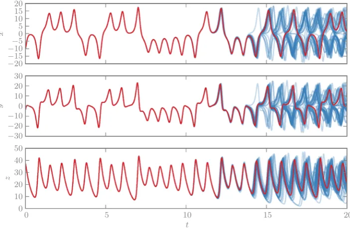
As a motivating example, consider the solution of the Lorenz’63 system. Since the problem is chaotic, any typi-cal fixed-step numeritypi-cal methods will become increasingly inaccurate for long integration times. Figure 1 depicts a deterministic solution for this problem, computed with a fixed-step, fourth-order, Runge–Kutta integrator. Although

the solver becomes completely inaccurate by the end of the depicted interval given the step-size selected, the solver pro-vides no obvious characterisation of its error at late times. Compare this with a sample of randomised solutions based on the same integrator and the same step-size; it is obvi-ous that early-time solutions are accurate and that they diverge at late times, reflecting instability of the solver. Every curve drawn has the same theoretical accuracy as the original classical method, but the randomised integra-tor provides a detailed and practical approach for revealing the sensitivity of the solution to numerical errors. The method used requires only a straightforward modification of the standard Runge–Kutta integrator and is explained in Sect.2.3.

We summarise the contributions of this work as follows:

– Construct randomised solvers of ODEs and PDEs using natural modification of popular, existing solvers. – Prove the convergence of the randomised methods and

study their behaviour by showing a close link between randomised ODE solvers and stochastic differential equations (SDEs).

– Demonstrate that these randomised solvers can be used to perform statistical analyses that appropriately consider solver uncertainty.

1.2 Review of existing work

The statistical analysis of models based on ordinary and partial differential equations is growing in importance and

Fig. 1 A comparison of solutions to the Lorenz’63 system using deterministic (red) and randomised (blue) integrators based on a fourth-order Runge–Kutta

integrator ₋−₂₀15

−−105 0 5 10 15 20

x

−30 −20 −100 10 20 30

y

0 5 10 15 20

t

0 10 20 30 40 50

a number of recent papers in the statistics literature have sought to address certain aspects specific to such mod-els, e.g. parameter estimation (Liang and Wu 2008; Xue et al. 2010; Xun et al. 2013; Brunel et al. 2014) and sur-rogate construction (Chakraborty et al. 2013). However, the statistical implications of the reliance on a numeri-cal approximation to the actual solution of the differential equation have not been addressed in the statistics litera-ture to date and this is the open problem comprehensively addressed in this paper. Earlier work in the literature includ-ing randomisation in the approximate integration of ordi-nary differential equations (ODEs) includes (Coulibaly and Lécot 1999; Stengle 1995). Our strategy fits within the emerging field known as Probabilistic Numerics (Hennig et al. 2015), a perspective on computational methods pio-neered byDiaconis(1988), and subsequently (Skilling 1992). This framework recasts solving differential equations as a statistical inference problem, yielding a probability mea-sure over functions that satisfy the constraints imposed by the specific differential equation. This measure formally quantifies the uncertainty in candidate solution(s) of the differential equation, allowing its use in uncertainty quan-tification (Sullivan 2016) or Bayesian inverse problems (Dashti and Stuart 2016).

A recent Probabilistic Numerics methodology for ODEs (Chkrebtii et al. 2013) [explored in parallel inHennig and Hauberg(2014)] has two important shortcomings. First, it is impractical, only supporting first-order accurate schemes with a rapidly growing computational cost caused by the growing difference stencil [althoughSchober et al.(2014) extends to Runge–Kutta methods]. Secondly, this method does not clearly articulate the relationship between their probabilistic structure and the problem being solved. These methods construct a Gaussian process whose mean coin-cides with an existing deterministic integrator. While they claim that the posterior variance is useful, by the con-jugacy inherent in linear Gaussian models, it is actually just an a priori estimate of the rate of convergence of the integrator, independent of the actual forcing or ini-tial condition of the problem being solved. These works also describe a procedure for randomising the construc-tion of the mean process, which bears similarity to our approach, but it is not formally studied. In contrast, we formally link each draw from our measure to the analytic solution.

Our motivation for enhancing inference problems with models of discretisation error is similar to the more gen-eral concept of model error, as developed byKennedy and O’Hagan (2001). Although more general types of model error, including uncertainty in the underlying physics, are important in many applications, our focus on errors aris-ing from the discretisation of differential equations leads to more specialised methods. Future work may be able to

trans-late insights from our study of the restricted problem to the more general case. Existing strategies for discretisation error include empirically fitted Gaussian models for PDE errors (Kaipio and Somersalo 2007) and randomly perturbed ODEs (Arnold et al. 2013); the latter partially coincides with our construction, but our motivation and analysis are distinct. Recent work (Capistrán et al. 2013) uses Bayes factors to analyse the impact of discretisation error on posterior approx-imation quality. Probabilistic models have also been used to study error propagation due to rounding error; see Hairer et al.(2008).

1.3 Organisation

The remainder of the paper has the following structure: Sect.2introduces and formally analyses the proposed proba-bilistic solvers for ODEs. Section3explores the characteris-tics of random solvers employed in the statistical analysis of both forward and inverse problems. Then, we turn to elliptic PDEs in Sect.4, where several key steps of the construction of probabilistic solvers and their analysis have intuitive ana-logues in the ODE context. Finally, an illustrative example of an elliptic PDE inference problem is presented in Sect.5.1

2 Probability measures via probabilistic time

integrators

Consider the following ordinary differential equation (ODE):

du

dt = f(u), u(0)=u0, (1)

where u(·) is a continuous function taking values in Rn.2 We letΦt denote the flow map for Eq. (1), so thatu(t) = Φt

u(0). The conditions ensuring that this solution exists will be formalised in Assumption2, below.

Deterministic numerical methods for the integration of this equation on time interval[0,T]will produce an approx-imation to the equation on a mesh of points{tk =kh}Kk₌0, withK h=T, (for simplicity we assume a fixed mesh). Let

uk=u(tk)denote the exact solution of (1) on the mesh and

Uk ≈ uk denote the approximation computed using finite evaluations of f. Typically, these methods output a single discrete solution{Uk}_kK₌₀, often augmented with some type of error indicator, but do not statistically quantify the uncer-tainty remaining in the path.

1 _{Supplementary materials and code are available online:http://www2.}

warwick.ac.uk/pints.

2 _{To simplify our discussion we assume that the ODE is autonomous,}

Let Xa_,b denote the Banach space C([a,b];Rn). The exact solution of (1) on the time interval[0,T]may be viewed as a Dirac measureδuonX0,Tat the elementuthat solves the ODE. We will construct a probability measureμhonX0_,T, that is straightforward to sample from both on and off the mesh, for whichh quantifies the size of the discretisation step employed, and whose distribution reflects the uncer-tainty resulting from the solution of the ODE. Convergence of the numerical method is then related to the contraction of μh_toδ

u.

We briefly summarise the construction of the numerical method. LetΨh : Rn → Rn denote a classical determin-istic one-step numerical integrator over time-steph, a class including all Runge–Kutta methods and Taylor methods for ODE numerical integration (Hairer et al. 1993). Our numer-ical methods will have the property that, on the mesh, they take the form

Uk₊1=Ψh(Uk)+ξk(h), (2)

whereξk(h)are suitably scaled, i.i.d. Gaussian random vari-ables. That is, the random solution iteratively takes the standard step,Ψh, followed by perturbation with a random draw,ξk(h), modelling uncertainty that accumulates between mesh points. The discrete path{Uk}_kK₌₀is straightforward to sample and in general is not a Gaussian process. Furthermore, the discrete trajectory can be extended into a continuous time approximation of the ODE, which we define as a draw from the measureμh.

The remainder of this section develops these solvers in detail and proves strong convergence of the random solu-tions to the exact solution, implying that μh → δu in an appropriate sense. Finally, we establish a close relationship between our random solver and a stochastic differential equa-tion (SDE) with small mesh-dependent noise. Intuitively, adding Gaussian noise to an ODE suggests a link to SDEs. Additionally, note that the mesh-restricted version of our algorithm, given by (2), has the same structure as a first-order Ito–Taylor expansion of the SDE

du = f(u)dt+σdW, (3)

for some choice ofσ. We make this link precise by perform-ing a backwards error analysis, which connects the behaviour of our solver to an associated SDE.

2.1 Probabilistic time integrators: general formulation

The integral form of Eq. (1) is

u(t)=u0+

t

fu(s)ds. (4)

The solutions on the mesh satisfy

uk+1=uk+

tk+1

tk

fu(s)ds, (5)

and may be interpolated between mesh points by means of the expression

u(t)=uk+

t

tk

fu(s)ds, t ∈ [tk,tk+1). (6)

We may then write

u(t)=uk+

t

tk

g(s)ds, t∈ [tk,tk+1), (7)

whereg(s)= fu(s)is an unknown function of time. In the algorithmic setting, we have approximate knowledge about

g(s)through an underlying numerical method. A variety of traditional numerical algorithms may be derived based on approximation ofg(s)by various simple deterministic func-tionsgh(s). The simplest such numerical method arises from

invoking the Euler approximation that

gh(s)= f(Uk), s∈ [tk,tk+1). (8)

In particular, if we taket =tk+1and apply this method induc-tively the corresponding numerical scheme arising from making such an approximation to g(s)in (7) is Uk+1 =

Uk + h f(Uk). Now consider the more general one-step numerical method Uk₊1 = Ψh(Uk). This may be derived by approximatingg(s)in (7) by

gh(s)= d

dτ

Ψτ(Uk)

τ=s−tk

, s∈ [tk,tk+1). (9)

We note that all consistent (in the sense of numerical analysis) one-step methods will satisfy

d dτ

Ψτ(u)

τ=0= f(u).

The approach based on the approximation (9) leads to a deterministic numerical method which is defined as a con-tinuous function of time. Specifically, we have U(s) =

Ψs−tk(Uk), s∈ [tk,tk+1).Consider again the Euler

approx-imation, for which Ψ_τ(U) = U + τf(U), and whose

s ∈ [tk,tk₊1).We propose to approximate gstochastically in order to represent this uncertainty, taking

gh(s)= d

dτ

Ψτ(Uk)

τ=s−tk

+χk(s−tk), s∈ [tk,tk+1)

where the{χk}form an i.i.d. sequence of Gaussian random functions defined on[0,h]withχk ∼N(0,Ch).3

We will chooseChto shrink to zero withhat a prescribed rate (see Assumption1), and also to ensure thatχk ∈ X0,h almost surely. The functions{χk}represent our uncertainty about the functiong. The corresponding numerical scheme arising from such an approximation is given by

Uk+1=Ψh(Uk)+ξk(h), (10)

where the i.i.d. sequence of functions{ξk}lies inX0,hand is given by

ξk(t)=

t

0

χk(τ)dτ. (11)

Note that the numerical solution is now naturally defined between grid points, via the expression

U(s)=Ψs−tk(Uk)+ξk(s−tk), s∈ [tk,tk+1). (12)

When it is necessary to evaluate a solution at multiple points in an interval,s ∈ (tk,tk+1], the perturbations ξk(s−tk) must be drawn jointly, which is facilitated by their Gaussian structure. Although most users will only need the formulation on mesh points, we must consider off-mesh behaviour to rigorously analyse higher order methods, as is also required for the deterministic variants of these methods.

In the case of the Euler method, for example, we have

Uk₊1=Uk+h f(Uk)+ξk(h) (13)

and, between grid points,

U(s)=Uk +(s−tk)f(Uk)+ξk(s−tk), s∈ [tk,tk+1). (14)

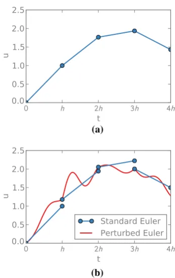
This method is illustrated in Fig.2. Observe that Eq. (13) has the same form as an Euler–Maryama method for an associated SDE (3) whereσ depends on the step-sizeh. In particular, in the simple one-dimensional case,σ would be given byCh_{/h. Section2.4develops a more sophisticated} connection that extends to higher order methods and off the mesh.

3_{We useχ}

k ∼ N(0,Ch)to denote a zero-mean Gaussian process

defined on[0,h]with a covariance kernel cov(χk(t), χk(s))Ch(t,s).

(a)

(b)

Fig. 2 An illustration of deterministic Euler steps and randomised vari-ations. The random integrator in (b) outputs the path in red; we overlay the standard Euler step constructed at each step, before it is perturbed (blue)

While we argue that the choice of modelling local uncer-tainty in the flow map as a Gaussian process is natural and analytically favourable, it is not unique. It is possi-ble to construct examples where the Gaussian assumption is invalid; for example, when a highly inadequate time-step is used, a systemic bias may be introduced. However, in regimes where the underlying deterministic method per-forms well, the centred Gaussian assumption is a reasonable prior.

2.2 Strong convergence result

To prove the strong convergence of our probabilistic numeri-cal solver, we first need two assumptions quantifying proper-ties of the random noise and of the underlying deterministic integrator, respectively. In what follows we use·,·and| · | to denote the Euclidean inner product and norm onRn. We denote the Frobenius norm onRn×nby| · |F, andEhdenotes expectation with respect to the i.i.d. sequence{χk}.

Assumption 1 Letξk(t):=

t

0χk(s)dswithχk∼N(0,Ch).

Then there existsK >0,p ≥1 such that, for allt ∈ [0,h],

Eh_|ξ

k(t)ξk(t)T|2F ≤ K t2p+1; in particular Eh|ξk(t)|2 ≤

K t2p+1. Furthermore, we assume the existence of matrix

Here, and in the sequel,Kis a constant independent ofh, but possibly changing from line to line. Note that the covari-ance kernelChis constrained, but not uniquely defined. We will assume the form of the constant matrix isQ=σI, and we discuss one possible strategy for choosingσ in Sect.3.1. Section2.4uses a weak convergence analysis to argue that onceQis selected, the exact choice ofChhas little practical impact.

Assumption 2 The function f and a sufficient number of its derivatives are bounded uniformly inRn in order to ensure that f is globally Lipschitz and that the numerical flow map Ψhhas uniform local truncation error of orderq+1:

sup

u∈Rn|Ψ

t(u)−Φt(u)| ≤K tq+1.

Remark 2.1 We assume globally Lipschitz f, and bounded derivatives, in order to highlight the key probabilistic ideas, whilst simplifying the numerical analysis. Future work will address the non-trivial issue of extending of analyses to weaken these assumptions. In this paper, we provide numer-ical results indicating that a weakening of the assumptions is indeed possible.

Theorem 2.2 Under Assumptions1,2it follows that there is K>0such that

sup

0≤kh≤T

Eh_|

uk−Uk|2≤K h2 min{p,q}.

Furthermore,

sup

0≤t≤T

Eh_{|u(t)−U(t)| ≤K h}min{p,q}_.

This theorem implies that every probabilistic solution is a good approximation of the exact solution in both a discrete and continuous sense. Choosingp≥q is natural if we want to preserve the strong order of accuracy of the underlying deterministic integrator; we proceed with the choicep =q, introducing the maximum amount of noise consistent with this constraint.

2.3 Examples of probabilistic time integrators

The canonical illustration of a probabilistic time integrator is the probabilistic Euler method already described.4Another useful example is the classicalRunge–Kutta methodwhich defines a one-step numerical integrator as follows:

Ψh(u)=u+

h

6

k1(u)+2k2(u,h)+2k3(u,h)+k4(u,h)

,

4_{An additional example of a probabilistic integrator, based on a}

Ornstein–Uhlenbeck process, is available in the supplementary materi-als.

where

k1(u)= f(u), k2(u,h)= f

u+1

2hk1(u)

k3(u,h)= f

u+1

2hk2(u)

, k4(u,h)= f

u+hk3(u)

.

The method has local truncation error in the form of Assump-tion2withq =4.It may be used as the basis of a probabilistic numerical method (12), and hence (10) at the grid points. Thus, provided that we choose to perturb this integrator with a random processχk satisfying Assumption1withp ≥4,5 Theorem2.2shows that the error between the probabilistic integrator based on the classical Runge–Kutta method is, in the mean square sense, of the same order of accuracy as the deterministic classical Runge–Kutta integrator.

2.4 Backward error analysis

Backwards error analyses are useful tool for numerical analy-sis; the idea is to characterise the method by identifying a modified equation (dependent upon h) which is solved by the numerical method either exactly, or at least to a higher degree of accuracy than the numerical method solves the original equation. For our random ODE solvers, we will show that the modified equation is a stochastic differential equation (SDE) in which only the matrixQfrom Assumption1enters; the details of the random processes used in our construction do not enter the modified equation. This universality prop-erty underpins the methodology we introduce as it shows that many different choices of random processes all lead to the same effective behaviour of the numerical method.

We introduce the operatorsLandLh_{defined so that, for} allφ∈C∞(Rn,R),

φΦh(u)

=ehLφ(u), EφU1|U0=u

=ehLhφ(u).

(15)

Thus L := f · ∇ andehLh is the kernel for the Markov chain generated by the probabilistic integrator (2). In fact we never need to work withLhitself in what follows, only with

ehLh_{, so that questions involving the operator logarithm do} not need to be discussed.

We now introduce a modified ODE and a modified SDE which will be needed in the analysis that follows. The mod-ified ODE is

duˆ

dt = f

h_(ˆ

u) (16)

5 _{Implementing Eq.10is trivial, since it simply adds an appropriately}

whilst the modified SDE has the form

du˜ = fh(u˜)dt+h2p_{QdW. (17)}

The precise choice of fhis detailed below. LettingEdenote expectation with respect toW, we introduce the operatorsLh andLhso that, for allφ∈C∞(Rn,R),

φuˆ(h)| ˆu(0)=u=ehLhφ(u), (18)

Eφu˜(h)| ˜u(0)=0=ehLhφ(u). (19)

Thus,

Lh_{:= f}h_{· ∇, L}h _{= f}h_{· ∇ +}1 2h

2p_{Q: ∇∇, (20)}

where:denotes the inner product onRn×nwhich induces the Frobenius norm, that is,A:B=trace(AT_B).

The fact that the deterministic numerical integrator has uniform local truncation error of orderq+1 (Assumption2) implies that, sinceφ∈C∞,

ehLφ(u)−φ(Ψh(u))=O(hq+1). (21)

The theory of modified equations for classical one-step numerical integration schemes for ODEs (Hairer et al. 1993) establishes that it is possible to find fhin the form

fh:= f +

q+l

i=q

hifi, (22)

such that

ehLhφ(u)−φ(Ψh(u))=O(hq+2+l). (23)

We work with this choice of fhin what follows. Now for our stochastic numerical method we have

φ(Uk+1)=φ(Ψh(Uk))+ξk(h)· ∇φ(Ψh(Uk)) +1

2ξk(h)ξ T

k (h): ∇∇φ(Ψh(Uk))+O(|ξk(h)|3).

Furthermore, the last term has mean of size O(|ξk(h)|4). From Assumption 1 we know that Ehξk(h)ξkT(h)

=

Qh2p+1.Thus

ehLhφ(u)−φΨh(u)

= 1

2h

2p₊1

Q: ∇∇φΨh(u)

+O(h4p+2). (24)

From this it follows that

ehLhφ(u)−φΨh(u)

= 1

2h

2p₊1

Q: ∇∇φ(u)+O(h2p+2). (25)

Finally we note that (20) implies that

ehLhφ(u)−ehLhφ(u)

=ehLhe12h2p+1Q:∇∇−_Iφ(_u)

=ehLh

₁

2h

2p+1

Q: ∇∇φ(u)+O(h4p+2)

=I+O(h)1

2h

2p+1

Q: ∇∇φ(u)

+O(h4p+2)

.

Thus we have

ehLhφ(u)−ehLhφ(u)= 1

2h

2p+1

Q: ∇∇φ(u)+O(h2p+2).

(26)

Now using (23), (25), and (26) we obtain

ehLhφ(u)−ehLhφ(u)=O(h2p+2)+O(hq+2+l). (27)

Balancing these terms, in what follows we make the choice

l =2p−q. Ifl <0 we adopt the convention that the drift

fhis simply f.With this choice ofqwe obtain

ehLhφ(u)−ehLhφ(u)=O(h2p+2). (28)

This demonstrates that the error between the Markov ker-nel of one-step of the SDE (17) and the Markov kernel of the numerical method (2) is of orderO(h2p+2). Some

straight-forward stability considerations show that the weak error over anO(1)time interval is O(h2p+1). We make assumptions giving this stability and then state a theorem comparing the weak error with respect to the modified Eq. (17), and the original Eq. (1).

Assumption 3 The function f is inC∞ and all its deriv-atives are uniformly bounded on Rn. Furthermore, f is such that the operators ehL and ehLh satisfy, for allψ ∈

C∞(Rn,R)and someL >0,

sup

u_∈Rn|

ehLψ(u)| ≤(1+Lh) sup

u_∈Rn|ψ(

u)|,

sup

u∈Rn|

ehLhψ(u)| ≤(1+Lh) sup

u∈Rn|ψ(

u)|.

aspects of the numerical analysis to a minimum. More sophis-ticated, but structurally similar, analysis would be required for weaker assumptions on f. Similar considerations apply to the assumptions onφ.

Theorem 2.4 Consider the numerical method (10) and assume that Assumptions1 and 3 are satisfied. Then, for

φ∈C∞function with all derivatives bounded uniformly on

Rn_{, we have that}

|φ(u(T))−Ehφ(Uk)

| ≤K hmin{2p,q}, kh=T,

and

|Eφ(u˜(T))−Ehφ(Uk)

| ≤K h2p+1, kh=T,

where u andu solve˜ (1)and(17), respectively.

Example 2.5 Consider the probabilistic integrator derived from the Euler method in dimensionn = 1. We thus have

q =1, and we hence set p =1. The results inHairer et al.

(2006) allow us to calculate fhwithl =1. The preceding theory then leads to strong order of convergence 1, measured relative to the true ODE (1), and weak order 3 relative to the SDE

duˆ =

f(uˆ)−h

2 f

_(uˆ)f(uˆ)+h2 12

f(uˆ)f2(uˆ)

+4(f(uˆ))2f(uˆ)dt+√C hdW.

These results allow us to constrain the behaviour of the randomised method using limited information about the covariance structure,Ch. The randomised solution converges weakly, at a high rate, to a solution that only depends onQ. Hence, we conclude that the practical behaviour of the solu-tion is only dependent upon Q, and otherwise,Ch may be any convenient kernel. With these results now available, the following section provides an empirical study of our proba-bilistic integrators.

3 Statistical inference and numerics

This section explores applications of the randomised ODE solvers developed in Sect.2 to forward and inverse prob-lems. Throughout this section, we use the FitzHugh–Nagumo model to illustrate ideas (Ramsay et al. 2007). This is a two-state non-linear oscillator, with two-states(V,R)and parameters (a,b,c), governed by the equations

dV

dt =c

V− V

3

3 +R

, dR dt = −

1

c(V−a+b R) .

(29)

This particular example does not satisfy the stringent Assumptions2and3and the numerical results shown demon-strate that, as indicated in Remarks2.1and2.3, our theory will extend to weaker assumptions on f, something we will address in future work.

3.1 Calibrating forward uncertainty propagation

Consider Eq. (29) with fixed initial conditions V(0) =

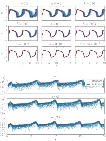
−1,R(0) = 1, and parameter values (.2, .2,3). Figure 3

shows draws of theV species trajectories from the measure associated with the probabilistic Euler solver with p=q =

1, for various values of the step-size and fixed σ = 0.1. The random draws exhibit non-Gaussian structure at large step-size and clearly contract towards the true solution.

Although the rate of contraction is governed by the underlying deterministic method, the scale parameter, σ, completely controls the apparent uncertainty in the solver.6 This tuning problem exists in general, since σ is problem dependent and cannot obviously be computed analytically.

Therefore, we propose to calibrate σ to replicate the amount of error suggested by classical error indicators. In the following discussion, we often explicitly denote the depen-dence onhandσ with superscripts, hence the probabilistic solver isUh,σ and the corresponding deterministic solver is

Uh,0. Define the deterministic error ase(t)=u(t)−Uh,0(t).

Then we assume there is some computable error indicator

E(t)≈e(t), defining Ek =E(tk). The simplest error indi-cators might compare differing step-sizes,E(t)=Uh,0(t)− U2h,0_{(t), or differing order methods, as in a Runge–Kutta 4–} 5 scheme.

We proceed by constructing a probability distribution π(σ )that is maximised when the desired matching occurs. We estimate this scale matching by comparing: (i) a Gaussian approximation of our random solver at each stepk,μ˜h_k,σ = N(E(U_kh,σ),V(U_kh,σ));and (ii) the natural Gaussian mea-sure from the deterministic solver,U_kh,0, and the available error indicator, Ek, ν_kσ = N(U_kh,0, (Ek)2). We construct π(σ )by penalising the distance between these two normal distributions at every step:π(σ )∝_kexp

−d(μ˜h_k,σ, ν_kσ)

. We find that the Bhattacharyya distance (closely related to the Hellinger metric) works well (Kailath 1967), since it diverges quickly if either the mean or variance differs. The density can be easily estimated using Monte Carlo. If the ODE state is a vector, we take the product of the univariate Bhattacharyya distances. Note that this calibration depends on the initial conditions and any parameters of the ODE.

6 _{Recall that throughout we assume that, within the context of}

Fig. 3 The true trajectory of theVspecies of the

FitzHugh–Nagumo model (red) and one hundred realisations from a probabilistic Euler ODE solver with various step-sizes

and noise scaleσ=.1 (blue) −4

−2 0 2 4

R

h

= 0

.

2

h

= 0

.

1

h

= 0

.

05

−4 −2 0 2 4

R

h

= 0

.

02

h

= 0

.

01

h

= 0

.

005

0 5 10 15 20

t

−4 −2 0 2 4

R

h

= 0

.

002

0 5 10 15 20

t

h

= 0

.

001

0 5 10 15 20

t

h

= 0

.

5

×

10

Fig. 4 A comparison of the error indicator for theVspecies of the FitzHugh–Nagumo model (blue) and the observed variation in the calibrated probabilistic solver. The red curves depict 50 samples of the magnitude of the difference between a standard Euler solver for several step-sizes and the equivalent randomised variant, usingσ∗, maximisingπ(σ)

Returning to the FitzHugh–Nagumo model, sampling from π(σ ) yields strongly peaked, uni-modal posteriors, hence we proceed using σ∗ = arg maxπ(σ ). We exam-ine the quality of the scale matching by plotting the magnitudes of the random variation against the error indi-cator in Fig. 4, observing good agreement of the mar-ginal variances. Note that our measure still reveals non-Gaussian structure and correlations in time not revealed by the deterministic analysis. As described, this procedure requires fixed inputs to the ODE, but it is straightfor-ward to marginalise out a prior distribution over input parameters.

3.2 Bayesian posterior inference problems

Given the calibrated probabilistic ODE solvers described above, let us consider how to incorporate them into infer-ence problems.

Assume we are interested in inferring parameters of the ODE given noisy observations of the state. Specifically, we wish to infer parametersθ∈Rdfor the differential equation

˙

u = f(u, θ), with fixed initial conditionsu(t =0)=u0(a straightforward modification may include inference on initial conditions). Assume we are provided with datad∈Rm,dj =

noise,ηj ∼N(0, Γ ). If we have priorQ(θ), the posterior we wish to explore is,P(θ | d) ∝ Q(θ)L(d,u(θ)),where densityLcompactly summarises this likelihood model.

The standard computational strategy is to simply replace the unavailable trajectory u with a numerical approxi-mation, inducing approximate posterior Ph,0(θ | d) ∝

Q(θ)L(d,Uh,0(θ)).Informally, this approximation will be accurate when the error in the numerical solver is small com-pared toΓand often converges formally toP(θ |d)ash →0 (Dashti and Stuart 2016). However, highly correlated errors at finitehcan have substantial impact.

In this work, we are concerned about the undue optimism in the predicted variance, that is, when the posterior concen-trates around an arbitrary parameter value even though the deterministic solver is inaccurate and is merely able to repro-duce the data by coincidence. The conventional concern is that any error in the solver will be transferred into posterior bias. Practitioners commonly alleviate both concerns by tun-ing the solver to be nearly perfect, however, we note that this may be computationally prohibitive in many contemporary statistical applications.

We can construct a different posterior that includes the uncertainty in the solver by taking an expectation over ran-dom solutions to the ODE

Ph,σ_{(θ |}

d)∝Q(θ)

L(d,Uh,σ(θ, ξ))dξ, (30)

whereUh,σ(θ, ξ)is a draw from the randomised solver given parametersθ and random drawξ. Intuitively, this construc-tion favours parameters that exhibit agreement with the entire family of uncertain trajectories. The typical effect of this expectation is to increase the posterior uncertainty onθ, pre-venting the inappropriate posterior collapse we are concerned about. Indeed, if the integrator cannot resolve the underlying dynamics,hp+1/2σ will be large. ThenUh,σ(θ, ξ)is inde-pendent ofθ, hence the prior is recovered,Ph,σ(θ | d) ≈

Q(θ).

Notice that ash → 0, both the measuresPh,0andPh,σ typically collapse to the analytic posterior,P, hence both methods are correct. We do not expect the bias ofPh,σ to be improved, since all of the averaged trajectories are of the same quality as the deterministic solver inPh,0. We now construct an analytic inference problem demonstrating these behaviours.

Example 3.1 Consider inferring the initial condition,u0 ∈

R, of the scalar linear differential equation, u˙ = λu,with λ >0.We apply a numerical method to produce the approx-imationUk ≈ u(kh). We observe the state at some times

t =kh, with additive noiseηk ∼N(0, γ2):dk =Uk+ηk. If we use a deterministic Euler solver, the model predicts

Uk =(1+hλ)ku0.These model predictions coincide with the slightly perturbed problem

du

dt =h

−1_log(1+λ

h)u,

hence error increases with time. However, the assumed obser-vational model does not allow for this, as the observation variance isγ2at all times.

In contrast, our proposed probabilistic Euler solver pre-dicts

Uk=(1+hλ)ku0+σh3/2

k−1

j=0

ξj(1+λh)k−j−1,

where we have made the natural choice p =q, whereσ is the problem-dependent scaling of the noise and theξk are i.i.d.N(0,1).For a single observation,ηkand everyξk are independent, so we may rearrange the equation to consider the perturbation as part of the observation operator. Hence, a single observation atkhas effective variance

γ2

h :=γ

2_+σ2

h3

k−1

j=0

(1+λh)2(k−j−1)

= γ2_+σ2

h3(1+λh)

2k₋₁

(1+λh)2₋₁.

Thus, late-time observations are modelled as being increas-ingly inaccurate.

Consider inferring u0, given a single observation dk at timek. If a Gaussian priorN(m0, ζ02)is specified for u0, then the posterior isN(m, ζ2), where

ζ−2₌ (1+hλ)2k γ2

h

+ζ−2

0 ,

ζ−2_m=(1+hλ)kdk γ2

h

+ζ−2

0 m0.

The observation precision is scaled by(1+hλ)2k because late-time data contain increasing information. Assume that the data aredk = eλkhu†₀+γ η†, for some given true ini-tial condition u†₀ and noise realisation η†. Consider now the asymptotic regime, whereh is fixed and k → ∞. For the standard Euler method, where γh = γ, we see that ζ2 _{→ 0, whilstm (1+hλ)}−1_ehλk_u†

0. Thus the infer-ence scheme becomes increasingly certain of the wrong answer: the variance tends to zero and the mean tends to infinity.

In contrast, with a randomised integrator, the fixedh, large

kasymptotics are

ζ2 1

ζ−2

0 +λ(2+λh)σ−2h−2

,

m

(1+hλ)−1ehλku†₀

Fig. 5 The posterior marginals of the FitzHugh–Nagumo inference problem using deterministic integrators with various step-sizes

h=.1 h=.05 h=.02 h=.01 h=.005

−0.2 0.0 0.2 0.4

0

.

1

0

.

2

θ1

2.6 2.8 3.0

−

0

.

2

0

.

0

0

.

2

0

.

4

θ2

2

.

6

2

.

8

3

.

0

θ3

Thus, the mean blows up at a modified rate, but the variance remains positive.

We take an empirical Bayes approach to choosingσ, that is, using a constant, fixed valueσ∗=arg maxπ(σ ), chosen before the data are observed. Joint inference of the parameters and the noise scale suffer from well-known MCMC mixing issues in Bayesian hierarchic models. To handle the unknown parameterθ, we can marginalise it out using the prior distrib-ution, or in simple problems, it may be reasonable to choose a fixed representative value.

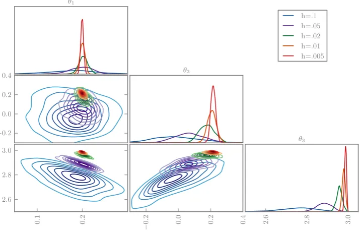
We now return to the FitzHugh–Nagumo model; given fixed initial conditions, we attempt to recover parameters θ = (a,b,c) from observations of both species at times τ =1,2, . . . ,40. The priors are log-normal, centred on the true value with unit variance, and with observational noise Γ =0.001. The data are generated from a high-quality solu-tion, and we perform inference using Euler integrators with various step-sizes,h ∈ {0.005,0.01,0.02,0.05,0.1}, span-ning a range of accurate and inaccurate integrators.

We first perform the inferences with naive use of deter-ministic Euler integrators. We simulate from each posterior using delayed rejection MCMC (Haario et al. 2006), shown in Fig. 5. Observe the undesirable concentration of every posterior, even those with poor solvers; the posteriors are almost mutually singular, hence clearly the posterior widths are meaningless.

Secondly, we repeat the experiment using our probabilis-tic Euler integrators, with results shown in Fig.6. We use a noisy pseudomarginal MCMC method, whose fast mix-ing is helpful for these initial experiments (Medina-Aguayo et al. 2015). These posteriors are significantly improved, exhibiting greater mutual agreement and obvious increasing

concentration with improving solver quality. The posteriors are not perfectly nested, possible evidence that our choice of scale parameter is imperfect, or that the assumption of locally Gaussian error deteriorates for large step-sizes. Note that the bias ofθ3is essentially unchanged with the randomised inte-grator, but the posterior for θ2 broadens and is correlated toθ3, hence introduces a bias in the posterior mode; with-out randomisation, only the inappropriate certainty abwith-outθ3 allowed the marginal forθ2to exhibit little bias.

4 Probabilistic solvers for partial differential

equations

We now turn to present a framework for probabilistic solu-tions to partial differential equasolu-tions, working within the finite element setting. Our discussion closely resembles the ODE case, except that now we randomly perturb the finite element basis functions.

4.1 Probabilistic finite element method for variational problems

LetVbe a Hilbert space of real-valued functions defined on a bounded polygonal domainD⊂Rd. Consider a weak for-mulation of a linear PDE specified via a symmetric bilinear forma:V×V −→R, and a linear formr :V −→Rto give the problem of findingu ∈ V : a(u, v) =r(v), ∀v ∈ V.

Fig. 6 The posterior marginals of the FitzHugh–Nagumo inference problem using probabilistic integrators with various step-sizes

h=.1 h=.05 h=.02 h=.01 h=.005

−0.2 0.0 0.2 0.4

0

.

1

0

.

2

θ1

2.6 2.8 3.0

−

0

.

2

0

.

0

0

.

2

0

.

4

θ2

2

.

6

2

.

8

3

.

0

θ3

U ∈Vh:a(U, v)=r(v), ∀v∈Vh. (31)

This is known as the Galerkin method.

We will work in the setting of finite element methods, assuming thatVh =span{φj}J_j=1, whereφj is locally sup-ported on a grid of points {xj}Jj₌1. The parameter h is introduced to measure the diameter of the finite elements. We will also assume that

φj(xk)=δj k. (32)

Any elementU∈Vhcan then be written as

U(x)=

J

j=1

Ujφj(x) (33)

from which it follows that U(xk) = Uk. The Galerkin method then gives AU = r, for U = (U1, . . . ,UJ)T,

Aj k =a(φj, φk), andrk =r(φk).

In order to account for uncertainty introduced by the numerical method, we will assume that each basis function φj can be split into the sum of a systematic partφsj and ran-dom partφr_j, where bothφjandφs_jsatisfy the nodal property (32), henceφr_j(xk)=0. Furthermore, we assume that each φr

jshares the same compact support as the correspondingφsj, preserving the sparsity structure of the underlying determin-istic method.

4.2 Strong convergence result

As in the ODE case, we begin our convergence analy-sis with assumptions constraining the random perturbations

and the underlying deterministic approximation. The bilin-ear forma(·,·)is assumed to induce an inner product, and then norm via · 2a = a(·,·); furthermore, we assume that this norm is equivalent to the norm on V. Through-out,Ehdenotes expectation with respect to the random basis functions.

Assumption 4 The collection of random basis functions {φr

j}

J

j=1 are independent, zero-mean, Gaussian random fields, each of which satisfies φr_j(xk) = 0 and shares the same support as the corresponding systematic basis function φs

j. For all j, the number of basis functions with index k which share the support of the basis functions with index

j is bounded independently ofJ, the total number of basis functions. Furthermore, the basis functions are scaled so that

J

j=1Ehφrj

2

a≤C h2p.

Assumption 5 The true solution u of problem (4.1) is in

L∞(D).Furthermore, the standard deterministic interpolant of the true solution, defined byvs:=J_j=1u(xj)φsj, satis-fiesu−vsa ≤C hq.

Theorem 4.1 Under Assumptions4and5it follows that the approximation U , given by(31), satisfies

Eh_u−U2

a≤C h2 min{p,q}.

4.3 Poisson solver in two dimensions

Consider a Poisson equation with Dirichlet boundary condi-tions in dimensiond=2, namely

−u= f, x∈ D, u=0, x∈∂D.

We setV =H₀1(D)andHto be the spaceL2(D)with inner product·,·and resulting norm| · |2 _{= ·,·.The weak} formulation of the problem has the form (4.1) with

a(u, v)=

D∇

u(x)∇v(x)dx, r(v)= f, v.

Now consider piecewise linear finite elements satisfying the assumptions of Sect. 4.2 inJohnson (2012) and take these to comprise the set{φs_j}J_j=1.Thenh measures the width of the triangulation of the finite element mesh. Assuming that

f ∈ Hit follows thatu ∈ H2(D)and that

u−vsa≤C huH2. (34)

Thusq =1. We choose random basis members{φr_j}J_j=1so that Assumption4hold withp=1. Theorem4.1then shows that, fore =u −U,Ehe2a ≤ C h2.We note that that in the deterministic case, we expect an improved rate of conver-gence in the function spaceH. Such a result can be shown to hold in our setting, following the usual arguments for the Aubin–Nitsche trickJohnson(2012), which is available in the supplementary materials.

5 PDE inference and numerics

We now perform numerical experiments using probabilistic solvers for elliptic PDEs. Specifically, we perform infer-ence in a 1D elliptic PDE, ∇ · (κ(x)∇u(x)) = 4x for

x ∈ [0,1], given boundary conditionsu(0)=0,u(1)=2. We represent logκ as piecewise constant over ten equal-sized intervals; the first, onx ∈ [0, .1)is fixed to be one to avoid non-identifiability issues, and the other nine are given a priorθi =logκi ∼ N(0,1). Observations of the fieldu are provided at x = (0.1,0.2, . . .0.9), with i.i.d. Gaussian error, N(0,10−5); the simulated observations were gener-ated using a fine grid and quadratic finite elements, then perturbed with error from this distribution.

Again we investigate the posterior produced at vari-ous grid sizes, using both deterministic and randomised solvers. The randomised basis functions are draws from a Brownian bridge conditioned to be zero at the nodal points, implemented in practice with a truncated Karhunen–Loève expansion. The covariance operator may be viewed as a frac-tional Laplacian, as discussed inLindgren et al.(2011). The scalingσis again determined by maximising the distribution described in Sect.3.1, where the error indicator compares lin-ear to quadratic basis functions, and we marginalise out the prior over theκi values.

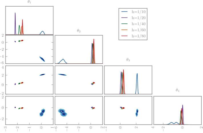
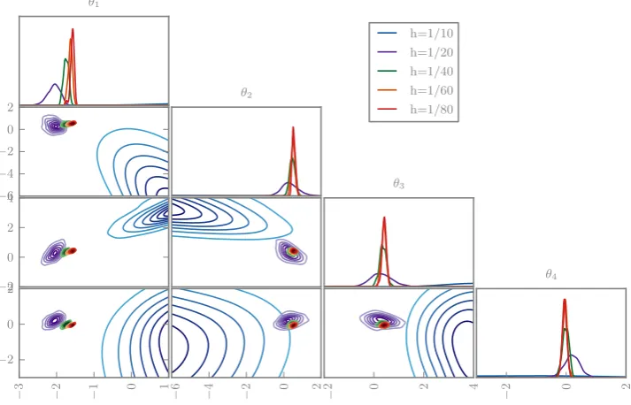
The posteriors are depicted in Figs.7and8. As in the ODE examples, the deterministic solvers lead to incompatible pos-teriors for varying grid sizes. In contrast, the randomised solvers suggest increasing confidence as the grid is refined, as desired. The coarsest grid size uses an obviously inade-quate ten elements, but this is only apparent in the randomised posterior.

Fig. 7 The marginal posterior distributions for the first four coefficients in 1D elliptic inverse problem using a classic deterministic solver with various grid sizes

h=1/10 h=1/20 h=1/40 h=1/60 h=1/80

−6

−4

−2 0 2

−2 0 2 4

−

3

−

2

−

1 0 1

θ1

−2 0 2

−

6

−

4

−

2 0 2

θ2

−

2 0 2 4

θ3

−

2 0 2

Fig. 8 The marginal posterior distributions for the first four coefficients in 1D elliptic inverse problem using a randomised solver with various grid sizes

h=1/10 h=1/20 h=1/40 h=1/60 h=1/80

−6

−4

−2 0 2

−2 0 2 4

−

3

−

2

−

1 0 1

θ1

−2 0 2

−

6

−

4

−

2 0 2

θ2

−

2 0 2 4

θ3

−

2 0 2

θ4

6 Conclusions

We have presented a computational methodology, backed by rigorous analysis, which enables quantification of the uncer-tainty arising from the finite-dimensional approximation of solutions of differential equations. These methods play a nat-ural role in statistical inference problems as they allow for the uncertainty from discretisation to be incorporated alongside other sources of uncertainty such as observational noise. We provide theoretical analyses of the probabilistic integrators which form the backbone of our methodology. Furthermore we demonstrate empirically that they induce more coher-ent inference in a number of illustrative examples. There are a variety of areas in the sciences and engineering which have the potential to draw on the methodology introduced including climatology, computational chemistry, and sys-tems biology.

Our key strategy is to make assumptions about thelocal

behaviour of solver error, which we have assumed to be Gaussian, and to draw samples from theglobaldistribution of uncertainty over solutions that results. Section2.4describes a universality result, simplifying task of choosing covariance kernels in practice, within the family of Gaussian processes. However, assumptions of Gaussian error, even locally, may not be appropriate in some cases, or may neglect important domain knowledge. Our framework can be extended in future work to consider alternate priors on the error, for example, multiplicative or non-negative errors.

Our study highlights difficult decisions practitioners face, regarding how to expend computational resources. While standard techniques perform well when the solver is highly

converged, our results show standard techniques can be dis-astrously wrong when the solver is not converged. As the measure of convergence is not a standard numerical analy-sis one, but a statistical one, we have argued that it can be surprisingly difficult to determine in advance which regime a particular problem resides in. Therefore, our practical rec-ommendation is that the lower cost of the standard approach makes it preferable when it is certain that the numerical method is strongly converged with respect to the statistical measure of interest. Otherwise, the randomised method we propose provides a robust and consistent approach to address the error introduced into the statistical task by numerical solver error. In difficult problem domains, such as numerical weather prediction, the focus has typically been on reducing the numerical error in each solver run; techniques such as these may allow a difference balance between numerical and statistical computing effort in the future.

The prevailing approach to model error described in

Acknowledgments The authors gratefully acknowledge support from EPSRC Grant CRiSM EP/D002060/1, EPSRC Established Career Research Fellowship EP/J016934/2, EPSRC Programme Grant EQUIP EP/K034154/1, and Academy of Finland Research Fellowship 266940. Konstantinos Zygalakis was partially supported by a grant from the Simons Foundation. Part of this work was done during the author’s stay at the Newton Institute for the program “Stochastic Dynamical Systems in Biology: Numerical Methods and Applications.;”

Open Access This article is distributed under the terms of the Creative Commons Attribution 4.0 International License (http://creativecomm ons.org/licenses/by/4.0/), which permits unrestricted use, distribution, and reproduction in any medium, provided you give appropriate credit to the original author(s) and the source, provide a link to the Creative Commons license, and indicate if changes were made.

A Numerical analysis details and proofs

Proof (Theorem2.2) We first derive the convergence result on the grid, and then in continuous time. From (10) we have

Uk₊1=Ψh(Uk)+ξk(h) (35)

whilst we know that

uk+1=Φh(uk). (36)

Define the truncation errork =Ψh(Uk)−Φh(Uk)and note that

Uk+1=Φh(Uk)+k+ξk(h). (37)

Subtracting Eq. (37) from (36) and definingek =uk−Uk, we get

ek+1=Φh(uk)−Φh(uk−ek)−k−ξk(h).

Taking the Euclidean norm and expectations give, using Assumption1and the independence of theξk,

Eh_|e

k+1|2=EhΦh(uk)−Φh(uk−ek)−k

2

+O(h2p+1),

where the constant in theO(h2p+1)term is uniform ink :

0 ≤ kh ≤ T.Assumption 2 implies thatk = O(hq+1), again uniformly ink : 0 ≤ kh ≤ T. Noting thatΦh is globally Lipschitz with constant bounded by 1+Lhunder Assumption2, we then obtain

Eh_|

ek+1|2≤(1+Lh)2Eh|ek|2 +Eh

h12Φ_h(_uk)−Φ_h(_uk−_ek),_h−12_k +O(h2q+2)+O(h2p+1).

Using Cauchy–Schwarz on the inner product, and the fact thatΦhis Lipschitz with constant bounded independently of

h, we get

Eh_|

ek₊1|2≤

1+O(h)Eh|ek|2+O(h2q+1)+O(h2p+1).

Application of the Gronwall inequality gives the desired result.

Now we turn to continuous time. We note that, for s ∈

[tk,tk+1),

U(s)=Ψs−tk(Uk)+ξk(s−tk),

u(s)=Φs−tk(uk).

LetFt denote theσ-algebra of events generated by the{ξk} up to timet. Subtracting we obtain, using Assumptions1and

2and the fact thatΦs−tk has Lipschitz constant of the form

1+O(h),

Eh_{|U(s)−u(s)|F}

tk

≤ |Φs−tk(Uk)−Φs−tk(uk)| + |Ψs₋tk(Uk)−Φs−tk(Uk)| +Eh_|ξ

k(s−tk)|Ftk

≤(1+Lh)|ek| +O(hq+1)+Eh|ξk(s−tk)| ≤(1+Lh)|ek| +O(hq+1)

+Eh_|ξ

k(s−tk)|2

1 2

≤(1+Lh)|ek| +O(hq+1)+O

hp+12

.

Now taking expectations we obtain

Eh_{|U(s)−u(s)| ≤(1+Lh)E}h_|e

k|2

1

2 +O(_hq+1) +Ohp+12

.

Using the on-grid error bound gives the desired result, after noting that the constants appearing are uniform in 0≤kh≤

T.

Proof (Theorem2.4) We prove the second bound first. Let wk =E

φ(u˜(tk))| ˜u(0)=u

andWk =Eh

φ(Uk)|U0=u). Then letδk =supu∈Rn|Wk−wk|.It follows from the Markov property that

Wk+1−wk+1=ehL h

Wk−ehL h

wk =ehLhWk−ehL

h

wk +ehLhwk−ehL

h

wk).

Using (28) and Assumption3we obtain

Iterating and employing the Gronwall inequality gives the second error bound.

Now we turn to the first error bound, comparing with the solutionuof the original Eq. (1). From (25) and then (21) we see that

ehLhφ(u)−φ(Ψh(u))=O(h2p+1),

ehLφ(u)−ehLhφ(u)=O(hmin{2p+1,q+1}).

This gives the first weak error estimate, after using the sta-bility estimate onehLfrom Assumption3.

Proof (Theorem 4.1) Recall the Galerkin orthogonality property which follows from subtracting the approximate variational principle from the true variational principle: it states that, fore=u−U,

a(e, v)=0, ∀v∈Vh. (38)

From this it follows that

ea≤ u−va, ∀v∈Vh. (39)

To see this note that, for anyv∈Vh, the orthogonality prop-erty (38) gives

a(e,e)=a(e,e+U−v)=a(e,u−v). (40)

Thus, by Cauchy–Schwarz,e2_a ≤ eau−va, ∀v ∈

Vh_{implying (39). We now set, forv∈V,}

v(x) =

J

j₌1

u(xj)φj(x)

= J

j=1

u(xj)φsj(x)+ J

j=1

u(xj)φrj(x)

=:vs_(x)+vr_(x).

By the mean-zero and independence properties of the random basis functions we deduce that

Eh_u−v2

a=Eha(u−v,u−v)

=Eh_a(u−vs_,u−vs_)+Eh_a(vr_{, v}r₎

= u−vs2_a+

J

j=1

u(xj)2Ehφrj 2

a.

The result follows from Assumptions4and5.

Ornstein–Uhlenbeck integrator

An additional example of a randomised integrator is an

integrated Ornstein–Uhlenbeck process, derived as follows. Define, on the intervals∈ [tk,tk+1), the pair of equations

dU=Vdt, U(tk)=Uk, (41a) dV = −ΛVdt+√2ΣdW, V(tk)= f(Uk). (41b)

Here W is a standard Brownian motion andΛ andΣ are invertible matrices, possibly depending onh. The approxi-mating functiongh(s)is thus defined byV(s), an Ornstein–

Uhlenbeck process.

Integrating (41b) we obtain

V(s)=exp−Λ(s−tk)

f(Uk)+χk(s−tk), (42)

wheres ∈ [tk,tk+1)and the{χk}form an i.i.d. sequence of Gaussian random functions defined on[0,h]with

χk(s)= √

2Σ

s

0

expΛ(τ−s)dW(τ).

Note that the h-dependence ofCh_{comes through the time} interval on whichχkis defined, and throughΛandΣ.

Integrating (41a), using (42), we obtain

U(s)=Uk+Λ−1

I −exp−Λ(s − tk)

f(Uk)

+ξk(s−tk), (43)

wheres∈ [tk,tk+1], and, fort∈ [0,h],

ξk(t)=

t

0

χk(τ)dτ. (44)

The numerical method (43) may be written in the form (12), and hence (10) at the grid points, with the definition

Ψh(u)=u+Λ−1

I−exp−Λhf(u).

This integrator is first-order accurate and satisfies Assump-tion2withp=1. Choosing to scaleΣwithhso thatq ≥1 in Assumption1leads to convergence of the numerical method with order 1.