Original citation:
Lokshtanov, Daniel, Ramanujan, Maadapuzhi Sridharan and Saket, Saurabh (2018) When
recursion is better than iteration : a linear-time algorithm for acyclicity with few error
vertices. In: 29th Annual ACM-SIAM Symposium on Discrete Algorithms, SODA 2018, New
Orleans, Louisiana, USA. , New Orleans, Louisiana, USA, 7-10 Jan 2018. Published in:
Proceedings of the Twenty-Ninth Annual ACM-SIAM Symposium on Discrete Algorithms pp.
1-18.
Permanent WRAP URL:
http://wrap.warwick.ac.uk/95237
Copyright and reuse:
The Warwick Research Archive Portal (WRAP) makes this work of researchers of the
University of Warwick available open access under the following conditions. Copyright ©
and all moral rights to the version of the paper presented here belong to the individual
author(s) and/or other copyright owners. To the extent reasonable and practicable the
material made available in WRAP has been checked for eligibility before being made
available.
Copies of full items can be used for personal research or study, educational, or not-for-profit
purposes without prior permission or charge. Provided that the authors, title and full
bibliographic details are credited, a hyperlink and/or URL is given for the original metadata
page and the content is not changed in any way.
Publisher’s statement:
First Published in Proceedings of the Twenty-Ninth Annual ACM-SIAM Symposium on
Discrete Algorithms 2018 published by the
Society for Industrial and Applied Mathematics (SIAM). Copyright © by SIAM. Unauthorized
reproduction of this article is prohibited.
A note on versions:
The version presented in WRAP is the published version or, version of record, and may be
cited as it appears here.
When Recursion is Better than Iteration: A Linear-Time Algorithm
for Acyclicity with Few Error Vertices
∗
Daniel Lokshtanov
†M. S. Ramanujan
‡Saket Saurabh
§†Abstract
Planarity, bipartiteness and (directed) acyclicity are basic graph properties with classic linear time recognition algo-rithms. However, the problems of testing whether a given (di)graph haskvertices whose deletion makes it planar, bi-partite or a directed acyclic graph (DAG) are all fundamental NP-complete problems whenk is part of the input. As a result, a significant amount of research has been devoted to understanding whether, for everyfixedk, these problems ad-mit a polynomial time algorithm (where the exponent in the polynomial is independent ofk) and in particular, whether they admit linear time algorithms.
While we now know that for any fixedk, we can test in linear time whether a graph is kvertices away from being planar [FOCS 2009, SODA 2014] or bipartite [SODA 2014, SICOMP 2016], the best known algorithms in the case of directed acyclicity are the algorithm of Garey and Tarjan [IPL 78] which runs in timeO(nk−1m) and the algorithm of Chen, Liu, Lu, O’Sullivan and Razgon [JACM 2008] which runs in timeO(k!4kk4nm). In other words, it has remained
open whether it is possible to recognize in linear time, a graph which is2 vertices away from being acyclic!
In this paper, we settle this question by giving an algorithm that decides whether a given graph iskvertices away from being acyclic, in timeO(k!4kk5(n+m)). That is,
for every fixedk, our algorithm runs in timeO(m+n), thus mirroring the case for planarity and bipartiteness.
Our algorithm is designed via a general methodology that shaves off a factor ofnfrom some algorithms that use the powerful technique of iterative compression. The two main features of our methodology are: (i) This is the first generic technique for designing linear time algorithms for
directed cut-problemsand (ii) it can be used in combination with future improvements in algorithms for thecompression
version of other well-studied cut-problems such asMulticut
∗Research supported byPareto-Optimal Parameterized
Algo-rithms, ERC Starting Grant 715744 andParameterized Approxi-mation, ERC Starting Grant 306992 andX-Tract, Austrian Science Fund (FWF, project P26696).
†University of Bergen, Norway,
‡University of Warwick, UK,
§The Institute of Mathematical Sciences, HBNI, India and UMI
ReLax,[email protected].
andDirected Subset Feedback Vertex Set.
1 Introduction
The classes of planar graphs, bipartite graphs and acyclic graphs are among the fundamental graph classes with seminal linear time recognition algorithms. However, the decision problem, that is, deciding whether there is a vertex set of size k(an outlier set) whoseremoval
places the input graph in a specific graph class is NP-complete for numerous basic graph classes, including the aforementioned three. As a result, a significant amount of research has been devoted to understanding whether, for every fixed k, these problems admit an algorithm with running timeO(nc) wherec is independent ofk (through the paradigm of fixed-parameter tractability and parameterized complexity) and if so, what the best possible value ofc is.
In fact, this area of research actually predates the area of parameterized complexity. The genesis of pa-rameterized complexity is in the theory of graph minors, developed by Robertson and Seymour [46,47,48]. Some of the important algorithmic consequences of this the-ory includeO(n3) algorithms for
Disjoint Pathsand
F-Deletionfor every fixed value of k. Another early work on obtaining algorithms with improved dependence on the input size was the seminal work of Bodlaender giving a linear time algorithm for Treewidth[2,3].
However, the advent of parameterized complexity started to shift the focus away from the running time dependence on input size to the dependence only on the parameter. That is, the goal became designing parameterized algorithms with running time upper bounded by f(k)nO(1), where the function f grows
as slowly as possible, without worrying about the polynomial dependence onnat all. But the last decade has witnessed several efforts aimed at obtaining linear time parameterized algorithms (or algorithms having the best possible dependence on the input size) that compromise as little as possible on the dependence of the running time on the parameterk. The gold standard for these results are algorithms with linear dependence on input size as well as provably optimal dependence on
the parameter under a complexity hypothesis such as the Exponential Time Hypothesis (ETH).
It was only relatively recently that the first linear time algorithms were obtained for testing whether a graph is k vertices away from being planar [33,25] or bipartite [31,43]. Some of the other important results in this line of research include the linear time algorithms forSubgraph Isomorphism[12],Subset Feedback Vertex Set[37], Planar F-Deletion[2,3,16,19,
18],Crossing Number[22,23,28],Interval Vertex Deletion [6], as well as a single-exponential and
linear time parameterized constant factor approximation algorithm for Treewidth [4]. In addition, there
are several recent results which provide parameterized algorithms with improved (but not linear) dependence on input size for a host of problems [24,26,27,34,29,30].
However, in spite of this progress, a linear time algorithm for testing whether a graph is k vertices away from being acyclic (for every fixed k), has still proved elusive. In fact, even the existence of a O(nc) algorithm for every fixedkwas widely posed as the most important open problem in parameterized complexity for well over a decade starting from the first few papers on fixed-parameter tractability (FPT) [13, 14]. In a break-through paper, Chen, Liu, Lu, O’Sullivan and Razgon [7] answered this question in the affirmative by proving that this problem, formally called Directed Feedback Vertex Set (DFVS) and defined below,
is fixed-parameter tractable (FPT). That is, it has an algorithm running in time f(k)nc for some computable functionf and a constantcindependent ofk.
Input: A digraphD onnvertices andmedges
and a positive integer k.
Parameter: k
Problem: Does there exist a vertex subset of size at mostk that intersects every cycle inD?
Directed Feedback Vertex Set (DFVS)
The algorithm of Chen et al. runs in time
O(4kk!k4n4) wherenis the number of vertices in the
in-put digraph. Subsequently, it was observed that, in fact, the running time of this algorithm isO(4kk!k4nm) (see
for example, [10]). That is, it runs in time O(mn) for every fixedk. On the other hand, Garey and Tarjan [21] gave an elegant algorithm for DFVS running in time
O(nk−1m) (as opposed to the trivialO(nk) algorithm). This algorithm clearly outperforms the algorithm of Chen et al. fork= 1 and runs in linear time. However, although the techniques used by Chen et al. have found numerous applications subsequently, it remained open whether one could detect in linear time, even a vertex
subset of size 2 that intersects every cycle in a given digraph!
In this paper we resolve this question (for every fixed
k) and obtain the first linear-time FPT algorithm for
DFVS. In particular we prove the following theorem.
Theorem 1.1. There is an algorithm for DFVS
run-ning in timeO(k!4kk5·(n+m)).
Our algorithm achieves the best possible dependence on the input size while matching the current best-known parameter-dependence – that of the algorithm of Chen et al. [7], up to a O(k) factor. Since it is well known that DFVS cannot be solved in time 2o(k)nc for any
constant c under the Exponential Time Hypothesis (ETH) [10, 11], our algorithm is in factnearly-optimal. Finally, our algorithm only relies on basic algorithmic and combinatorial tools.
Methodology. At the heart of numerous FPT algo-rithms lies the fact that, if one could efficiently compute a sufficiently good approximate solution, it is then suffi-cient to design an FPT algorithm for the “compression version” of a problem in order to obtain an FPT algo-rithm for the general version. In the compression version of a problem, the input also includes an approximate so-lution whose size depends only on the parameter. Since a given approximate solution may be used to infer signifi-cant structural information about the input, it is usually much easier to design FPT algorithms for the compres-sion vercompres-sion than for the original problem. The efficiency of this approach clearly depends on two factors – (a) the time required to compute an approximate solution and (b) the time required to solve the compression version of the problem when the approximate solution is provided as input.
This approach has been used mainly in the following two settings. In the first setting, the objective is the design of linear-time FPT algorithms. In this setting, for certain problems, it can be shown that if the treewidth of the input graph is bounded by a function of the parameter then the problem can be solved by a linear-time FPT algorithm (either designed explicitly or obtained by invocation of an appropriate algorithmic meta-theorem). On the other hand, if the treewidth of the input graph exceeds a certain bound, then there is a sufficiently large (induced) matching which one can contract and obtain an instance whosesize is a constant fraction of that of the original input. Now, the algorithm is recursively invoked on the reduced instance and certain problem-specific steps are used to convert the recursively computed solution into an approximate solution for the given instance. Then, a linear-time FPT algorithm for
the compression version is executed to solve the general problem on this instance. Some of the results that fall under this paradigm are Bodlaender’s linear FPT algorithm for Treewidth[3], the FPT-approximation
algorithms forTreewidth[4,44], as well as algorithms
forVertex Planarization[25,33]. Let us call this the
method ofrecursive compression. This is one of the most commonly used techniques in designing linear-time FPT-algorithms onundirected graphs. However, this approach of recursion combined with a win/win approach based on the treewidth of the graph, fails when one attempts to extend it to directed graphs.
On the other hand, when designing FPT algorithms where the dependence on the input isnotrequired to be linear, one can use the iterative compression technique, introduced by Reed, Smith and Vetta [45]. Here the input instance is gradually built up by simple operations, such as vertex additions. After each operation, an optimal solution is re-computed, starting from an optimal solution to the smaller instance. Though it is very helpful for problems on directed graphs, by its very definition, the iterative compression technique does not lend itself to the design of linear-time FPT algorithms. Hence, it appears that one has to look for alternative ways when aiming for linear-time FPT algorithms. In recent years, some of the problems which were initially solved using the iterative compression technique, have seen the development of entirely new algorithms. Examples include the first linear-time FPT algorithms for the Odd Cycle Transversal, Almost 2-SAT, Edge Unique Label Cover and Node Unique Label Coverproblems [31,43,32,38].
All of these algorithms are based on branching and linear programming techniques.
Another general approach to the design of linear-time FPT algorithms has been introduced by Marx et al. [39]. These algorithms are based on the “Treewidth Reduction Theorem”’ which states that in undirected graphs, for any pair of vertices sandt, all minimals-t
separators of bounded size are contained in a part of the graph that has bounded treewidth.
However, this technique is also specifically designed for undirected graphs and hence fails when addressing problems on directed graphs. Our main contribution is a novel approach for ‘lifting’ linear-time FPT algorithms for the compression version of feedback-set problems on digraphs to linear-time FPT algorithms for the general version of the problem. Although our approach follows the recursive compression paradigm pioneered by Bodlaender [3] in his celebrated linear time FPT algorithm for Treewidth, we need to identify highly
non-trivial structure in the given digraph to be even
able to compute the parts of the input digraph which we want to ‘recursively compress’.
Given a digraph D, we say that S is a directed feedback vertex set (dfvs)if deletingS fromD results in a DAG. At the core of our algorithm lies the following new structural lemma regarding digraphs with a small dfvs.
Lemma 1.1. LetD be a strongly connected digraph and p∈N. There is an algorithm that, given D and p, runs
in time O(p2m) (wheremis the number of arcs in D)
and either correctly concludes thatD has no dfvs of size at mostpor returns a setS with at most 2p+ 2 vertices such that one of the following holds.
• S is a dfvs forD.
• D−S has at least 2 non-trivial strongly connected components (strongly connected components with at least 2 vertices).
• The number of arcs of D whose head and tail occur in the same non-trivial strongly connected component of D−S (arcs participating in a cycle of D−S) is at most m2.
• If D has a dfvs of size at mostpthenD−S has a dfvs of size at most p−1.
Our linear-time FPT algorithm forDFVSis obtained by
a careful interleaving of the algorithm of Lemma1.1with an algorithm solving the compression version ofDFVS
(in this case, the compression routine of Chen et al. [7]). The proof of Lemma 1.1 itself is based on extending the notion of important sequences [36] to digraphs, and then analyzing a single such sequence. Furthermore, the proof of Lemma 1.1 only relies on properties of
DFVS that are shared by several other feedback set
and graph separation problems. Hence, we also prove a more general version of this lemma and show how it can be used as a black box to shave off a factor of n
from existing iterative compression based algorithms for other problems which satisfy certain conditions. This results in speeding up by a factor ofn, the current best FPT algorithms forMulticut[40,41,5] andDirected Subset Feedback Vertex Set[8,9].
2 Preliminaries
Parameterized Complexity. Formally, a parameteri-zation of a problem is the assignment of an integerk
to each input instance and we say that a parameterized problem isfixed-parameter tractable(FPT) if there is an algorithm that solves the problem in timef(k)· |I|O(1),
where|I| is the size of the input instance and f is an
arbitrary computable function depending only on the pa-rameterk. For more background, the reader is referred to the monographs [15, 17, 42,10].
Digraphs. For a digraphD and vertex setX⊆V(D), we say thatX is a dfvsofD ifX intersects every cycle inD. We say thatX is a minimal dfvs ofDif no proper subset ofX is also a dfvs ofD. We callX a minimum dfvs of D if there is no smaller dfvs of D. For an arc (u, v)∈ A(D), we refer to uas the tail of the arc and
v as thehead. D is a bidirectional digraph if for every (u, v) ∈ A(D), there is an arc (v, u) ∈ A(D). For a subsetX of vertices, we use N+(X) to denote the set
of out-neighbors of X and N−(X) to denote the set of in-neighbors ofX. We useNi[X] to denote the set
X∪Ni(X) wherei∈ {+,−}. We denote byA[X] the subset of A(D) with both endpoints inX. A strongly connected component of D is a maximal subgraph in which every vertex has a directed path to every other vertex. We say that a strongly connected component is non-trivial if it has at least 2 vertices and trivial
otherwise. For disjoint vertex setsX andY,Y is said to be reachable fromX if forevery vertexy∈Y, there is a vertexx∈X such that the digraph contains a directed path from xtoy.
Structures. For η ∈ N, an η-structure is a tuple where the first element of the tuple is a digraphD with the remaining elements of the tuple being relations of arity at mostη overV(D). Formally, anη-structure is a tuple (D, R1, . . . , R`) whereDis a digraph and for every
i∈[`],Ri⊆V(D)p for somep∈[η].
Two η-structures Q1 and Q2 are said to have
the same type if they both have the same number of elements and the corresponding relations have the same arity when non-empty. Formally, we say thatQ1
and Q2 have the same type if Q1 = (D1, R1, . . . , R`),
Q2= (D0, R01, . . . , R0`) and for eachi∈[`], there exists
p∈[η] such that, ifRi, R0i6=∅thenRi, R0i⊆V(D)pand
Ri, R0i6⊆V(D)p−1.
The size of an η-structure Q = (D, R1, . . . , R`) is denoted as |Q| and is defined asm+n+η·Σ`
i=1|Ri|, wheremandnare the number of arcs and vertices in
D respectively and|Ri| is the number of tuples inRi. In this paper, whenever we talk about a family Q of
η-structures, it is to be understood thatQonly contains
η-structures which are pairwise of the same type and this type is also called thetype ofQ.
Definition 1. Let Q = (D, R1, . . . , R`) be an η
-structure. For a setX ⊆V(D), we define the induced substructure Q[X] = (D[X], R1|X, . . . , R`|X) where
Ri|X is the restriction of the relation Ri to the set X,
that is, Ri|X =Ri∩(Sp∈[η]Xp). For any X ⊆V(D),
we denote by Q−X the substructureQ[V(D)\X].
Definition 2. Let Q be a family ofη-structures. We say thatQishereditaryif for everyQ∈ Q, every induced substructure of Q is also in Q. We say that a family
Q of η-structures islinear-time recognizable if there is an algorithm that, given anη-structureQ, runs in time
O(|Q|) and correctly decides whether Q∈ Q. Finally, we say that Q is rigid if the following two properties hold:
• For everyη-structureQ= (D, R1, . . . , R`), ifD has
no arcs thenQ∈ Q and
• Q = (D, R1, . . . , R`) ∈ Q if and only if for every
strongly connected component C in the digraphD, the induced substructure Q[C]∈ Q.
TheQ-Deletion(η)problem is formally defined as
follows.
Input: Anη-structureQ= (D, R1, . . . , R`) and a positive integer k.
Parameter: k
Problem: Does there exist a set X⊆V(D) of size at mostk such thatQ−X∈ Q?
Q-Deletion(η)
Our main contribution is a theorem (Theorem3.1) that, under certain conditions which are fulfilled by several well-studied special cases of Q-Deletion(η),
guarantees an FPT algorithm forQ-Deletion(η)whose
running time has a specific form.
A set X ⊆V(D) such that Q−X ∈ Q is called a deletion set of Q into Q. In the Q-Deletion(η) Compressionproblem, the input is a triple (Q, k,Wˆ)
where (Q, k) is an instance ofQ-Deletion(η)and ˆW
is a vertex set such that Q−Wˆ ∈ Q. The question remains the same as forQ-Deletion(η). However, the
parameter for this problem isk+|Wˆ|and for the input to be interesting, |Wˆ| > k (otherwise the instance is trivially aYesinstance). We say that an algorithmAis
an algorithm for the Q-Deletion(η) Compression
problem if, on input Q, k,Wˆ the algorithm either correctly concludes that (Q, k) is a No instance ofQ -Deletion(η) or computes a smallest set X of size
at most k such that Q−X ∈ Q. Note that the requirement that the setX is asmallestsuch set, does not affect generality for the following reason. Let A0
be an algorithm that, on inputQ, k,Wˆ either correctly concludes that (Q, k) is aNoinstance ofQ-Deletion(η)
or computes a (not necessarily smallest) setX of size at
mostksuch thatQ−X ∈ Q. We can then set ˆW0=X
and runA0 with inputQ, k−1,Wˆ0 to compute a smaller
solution if one exists and repeat this procedure (at most
k times) until we find a smallest such set. In this case, the running time of A is bounded by k times that of
A0. However, for all specific problems we address in this paper, we will not be required to take this route because the existing compression algorithms for DFVS, Multicut, andDirected Subset Feedback Vertex Set which we invoke can already be seen to output a
smallestset of size at mostk which is a solution.
3 The FPTalgorithm for Q-deletion(η)
In this section, we formally state our main theorem and demonstrate how a direct application of this theorem speeds up by a factor ofn, existing FPT algorithms for certain well-studied feedback set and graph separation problems. We then prove this theorem assuming a generalization of Lemma1.1as a black box.
Theorem 3.1. Let η ∈ N and let Q be a linear-time
recognizable, hereditary and rigid family ofη-structures. Let γ ∈N, d ∈R>1 and f :N→N such that f(t)≥t
andf(t−1)≤ fd(t) for everyt∈N.
• Let Abe an algorithm for Q-Deletion(η) Com-pression that, on input Q = (D, R1, . . . , R`), k
andWˆ, runs in timeO(f(k)· |Q|γ· |Wˆ|), whereWˆ
is a deletion set ofQintoQ,
• Let B be an algorithm that, on input Q = (D, R1, . . . , R`) ∈ Q/ , runs in time O(|Q|) and
re-turns a pair of verticesu, v such that every deletion set of Qinto Qwhich is disjoint from uand v is a u-v separator inD.
Then, there is an algorithm that, given an instance
(Q = (D, R1, . . . , R`), k) of Q-Deletion(η) and the algorithms A and B, runs in time O(f(k)·k· |Q|γ)
and either computes a set X of size at mostk such that Q−X ∈ Qor correctly concludes that no such set exists.
Before we proceed, we make a few remarks regarding the conditions in the premise of the theorem. Note that we require the running time of Algorithm A to be of the form O(f(k)· |Q|γ· |Wˆ|) in spite of the Q
-deletion(η) compression problem being formally
parameterized by|Wˆ|+k. At first glance, it may appear that this is a requirement that is much stronger than simply asking for an FPT algorithm for Q-deletion(η) compression. However, we point out that as long asQ
is hereditary, this requirement is in fact no stronger than simply asking for an FPT algorithm for Q-deletion(η) compression. Precisely, if there is an FPT algorithm
forQ-deletion(η) compression, that is an algorithm
that runs in timeO(g(k+|Wˆ|)· |Q|δ) for some function
g and constant δ, then we can obtain an algorithm for Q-deletion(η) compression that runs in time
O(g(2k+ 1)· |Q|δ · |Wˆ|) by using the folklore trick of running the compression step for the special case of
|Wˆ|=k+ 1, |Wˆ|times. This clearly suffices. We now illustrate the power of our theorem by applying it to a few well-studied problems.
3.1 Applications We describe how Theorem3.1can be invoked to shave off a factor of n from existing it-erative compression based algorithms for DFVS, Di-rected Feedback Arc Set(DFAS),Directed Sub-set Feedback Vertex Set and Multicut. Here, DFASis thearcdeletion version ofDFVSwhere the
ob-jective is to delete at mostkarcs from the given digraph to make it acyclic.
1. Application to DFVS. We setη = 1 and define
Q to be the set of all directed acyclic graphs. That is,
Q ={(D,∅) | Dis acyclic}. Clearly, Q is linear-time recognizable, hereditary and rigid. The algorithmBis defined to be an algorithm that, given as input a digraph
D which is not acyclic, simply picks an arc (a, b) which is part of a directed cycle inD and returnsu, v where
u=bandv=a. The algorithmAcan be chosen to be any compression routine for DFVS. In particular, we
choose the compression routine of Chen et al. [7] which runs in time O(f(k)(n+m)· |W|) wheref(k) = 4kk!k4.
Invoking Theorem3.1forQ-Deletion (1), we obtain
our linear-time algorithm for DFVS.
Theorem 3.2. There is an algorithm for DFVS run-ning in timeO(k!4kk5·(n+m)).
It is easy to see that DFAS can be reduced to DFVS in the following way. For an instance (D, k)
of DFAS, subdivide each arc, and make k+ 1 copies
of the original vertices to obtain a graph D0. It is straightforward to see that (D, k) is aYesinstance of DFVS if and only if (D0, k) is aYesinstance ofDFAS.
Since |D0| ≤2(k+ 1)|D|, we also obtain a linear-time
FPT algorithm forDFAS.
Corollary 3.1. There is an algorithm for DFAS
running in time O(k!4kk6·(n+m)).
2. Application to Multicut. In the Multicut
problem, the input is an undirected graph G, integerk
and pairs of vertices (s1, t1), . . . ,(sr, tr) and the objective is to check whether there is a set X of at most k
vertices such that for every i ∈ [r], si and ti are
in different connected components of G−X. The parameterized complexity of this problem was open for a long time until Marx and Razgon [41] and Bousquet, Daligault and Thomass´e [5] showed it to be FPT. Marx and Razgon obtained their FPT algorithm via the iterative compression technique. They gave an algorithm for the compression version ofMulticutthat,
on inputD,(s1, t1), . . . ,(sr, tr), k and ˆW, runs in time 2O(k3)
·nγ · |Wˆ| for some γ. As a result, they were able to obtain an algorithm for Multicut that runs
in time 2O(k3)
·nγ+1. Since the objective of Marx and
Razgon in their paper was to show the fixed-parameter tractability of Multicut, they did not try to optimize γ. However, going through the algorithm of Marx and Razgon and making careful (but standard) modifications of the derandomization step in their algorithm using Theorem 5.16 [10] (see also [1]) as well as the more recent linear time FPT algorithms for the Almost 2-SAT problem [43, 31] instead of the algorithm in
[35], it is possible to bound the running time of their compression routine by 2O(k3)
mnlogn and hence that of their algorithm by 2O(k3)
mn2logn. We now show by
an application of Theorem3.1that we can improve this running time by a factor ofn.
Set η = 2 and define Q to be the set of all pairs (D, S) where D is a bidirectional di-graph and S is the relation capturing the pairs to be separated. Formally, Q = {(D, S) |
D is bidirectional,S ⊆ V(D)2, ifS6=∅ then∀(u, v)∈ S, u andvare in distinct strongly connected
components of D}. Clearly, Q is linear-time recog-nizable, hereditary and rigid. We define A to be the compression routine of Marx and Razgon [41] andBto be an algorithm that computes the strongly connected components of D and simply returns a pair (u, v)∈S
(if it exists) such thatuandv are in the same strongly connected component of D. By invoking Theorem3.1 for Q-Deletion(2)with these parameters, we obtain the following corollary.
Corollary 3.2. There is an algorithm forMulticut
running in time 2O(k3)
mnlogn.
3. Application to Directed Subset Feedback
Vertex Set. In theDirected Subset Feedback Vertex Set(DSFVS) problem, the input is a digraph D, a setS of vertices inD and the objective is to check whether D contains a vertex set X of size at most k
such that D−X has no cycles passing throughS, also calledS-cycles. This problem is a clear generalization of
DFVSand was shown to be FPT by Chitnis et al. [9]
via the iterative compression technique.
They also observed that this problem is equivalent to theArc Directed Subset Feedback Vertex Set
(ADSFVS) where the input is a digraphDand a set S
of arcs in D and the objective is to check whether D
contains a vertex setX of size at mostksuch thatD−X
has no cycles passing through S. Chitnis et al. gave an algorithm for the compression version of ADSFVS that, on input D, S, k and ˆW, runs in time 2O(k3)
·nγ· |Wˆ| for some γ. As a result, they were able to obtain an algorithm for ADSFVS that runs in time 2O(k3)
·nγ+1.
We show by an application of Theorem3.1that we can directly shave off a factor of nfrom this running time.
We first argue that ADSFVS is a special case of Q -Deletion (2). We define byQthe set of all pairs (D, S)
whereS ⊆A(D) and D has no cycle passing through an arc in S. Clearly, Q is linear-time recognizable, hereditary and rigid. We defineAto be the compression routine of Chitnis et al. [9] andBto be an algorithm that, given as input the pair (D, S), computes the strongly connected components ofDand simply returns an arc in
S which is contained in a strongly connected component of D. By invoking Theorem 3.1 for Q-Deletion (2)
with these parameters, we obtain the following corollary.
Corollary 3.3. There is an algorithm for Arc Di-rected Subset Feedback Vertex Set running in
time2O(k3)
·nγ.
Due to the aforementioned observation of Chitnis et al., we also get an algorithm with the same running time forDirected Subset Feedback Vertex Set.
Having described the main applications of our theorem, we now proceed to its proof.
3.2 Proof of Theorem 3.1 The main technical component of the proof of this theorem is a generalization of Lemma 1.1. The proof of this lemma (Lemma3.1), is fairly technical and requires the introduction of more notation. For readers who are interested in a quick look at the central ideas behind the proof of Lemma3.1 without having to deal with the technical complications brought about by dealing with structures, we direct them to Section 4(for the relevant structural lemmas) and Section 5for a separate proof of Lemma1.1. We only state Lemma3.1 here and omit the proof due to space constraints.
Lemma 3.1. Let η ∈ N and let Q be a linear-time
recognizable, hereditary and rigid family ofη-structures. There is an algorithm that, given an η-structure Q = (D, R1, . . . , R`) ∈ Q/ where D is strongly connected,
vertices u, v ∈ V(D), and p ∈ N, runs in time
O(p2|Q|)and either correctly concludes thatD has no
u-v separator of size at mostpor returns a setS with at most 2p+ 2vertices such that one of the following holds.
• Q−S∈ Q.
• D−S has at least 2 strongly connected components each of which induces a substructure ofQnot inQ.
• The strongly connected components of D−S can be partitioned into 2 sets inducing substructures of Q, sayQ1 andQ2 such that Q1∈ Q/ ,Q2∈ Q and
|Q1| ≤ 12|Q|.
• IfQhas a deletion set of size at mostpintoQthen Q−S has a deletion set of size at mostp−1 into
Q.
We now return to Theorem3.1and proceed to prove it assuming this lemma as a black-box. We describe our algorithm forQ-deletion(η)using the algorithmsA, B and the algorithm of Lemma3.1as subroutines. The input to the algorithm in Theorem 3.1 is an instance (Q = (D, R1, . . . , R`), k) of Q-deletion(η) and the
output is No if Q has no deletion set into Q of size
at mostk and otherwise, the output is a setX which is a minimum sizedeletion set ofQintoQof size at most
k.
Description of the Algorithm of Theorem3.1and Correctness. We now give a formal description of the algorithm. The algorithm is recursive, each call takes as input an η-structureQ= (D, R1, . . . , R`) and integer
k. In the course of describing the algorithm we will also prove by induction onk+|Q|that the algorithm either correctly concludes thatQhas no deletion set intoQ of size at mostk, or finds a minimum size deletion set ofQ
intoQ, sayX of size at mostk. The algorithm proceeds as follows.
In time linear in the size of the digraph D, the algorithm computes the decomposition ofDinto strongly connected components. LetD0 be the digraph obtained
from D by removing from D all strongly connected components which induce a substructure of Qthat is already inQ. This operation is safe because the classQ
is rigid and hereditary. That is, ifQ0= (D0, R0
1, . . . , R0`) is the substructure of Q induced on V(D0) then any deletion set of Q intoQ is a deletion set ofQ0 intoQ
and vice versa. So the algorithm proceeds by working on
Q0 instead. For ease of description, we now revert back to the inputη-structureQ= (D, R1, . . . , R`) and assume without loss of generality thatD does not contain any trivial strongly connected components.
IfDis the empty graph or more generally, ifQ∈ Q, then the algorithm correctly returns the empty set as a minimum size deletion set ofQintoQ. From now on we assume thatD is non-empty. SinceD does not contain
any trivial strongly connected components this implies that m≥n≥2 and hence|Q| ≥2.
If k= 0 the algorithm correctly returns No, since Q /∈ Q. From now on we assume that k ≥ 1. For
k≥1, we determine from the computed decomposition of D into strongly connected components whether D
is strongly connected. If it is not, then let C be the vertex set of an arbitrarily chosen strongly connected component ofD. The algorithm calls itself recursively on the instances (Q[C], k−1) and (Q−C, k−1). If either of the recursive calls return No the algorithm
returnsNo as well since, bothQ[C] andQ−C need to
contain at least one vertex from any deletion set of Q
intoQ. Otherwise the recursive calls return setsX1and X2 such that X1 is a deletion set of Q[C] intoQ, X2
is a deletion set ofQ−C intoQand bothX1 andX2
have size at most k−1 each. The algorithm executes AlgorithmAon (Q,k) with ˆW =X1∪X2, and returns
the same answer as the Algorithm A. From now on we assume thatD is strongly connected.
For k ≥ 1 and strongly connected graph D the algorithm proceeds as follows. It starts by running the algorithmBonQto compute in timeO(|Q|) a pair of verticesu, v ∈V(D) such thatevery deletion set of Q
into Qwhich is disjoint fromuandv hits allu-v paths in D. Clearly,Q, u, v satisfy the premise of Lemma3.1. Hence we execute the subroutine described in Lemma3.1 onQ, u, v withp=k. Recall that the execution of this subroutine will have one of two possible outcomes. In the first case, the subroutine returns a setS ⊆V(D) of size at most 2k+ 2≤3ksatisfying one of the properties in the statement of Lemma3.1. In the second case, the subroutine concludes that D has no u-v separator of size at most p. But in this case, we infer that Qhas no deletion set into Q of size at most k disjoint from
{u, v}and hence we defineS to be the set{u, v}. Now, observe that this setStrivially satisfies the last property in the statement of Lemma3.1. Hence, irrespective of the outcome of the subroutine, we will have computed a setS of size at most 3k which satisfies one of the four properties in the statement of Lemma 3.1.
Observe that it is straightforward to check in linear time whether S satisfies any of the first 3 properties. Therefore, if none of these properties are satisfied, then we assume that S satisfies the last property. Furthermore, we work with the earliest property that
S satisfies. That is, if S satisfies Property i and Property j where 1≤ i < j ≤ 4 then we execute the steps corresponding to Casei. Subsequent steps of our algorithm will depend on the output of this check onS.
Case 1: Q−S∈ Q. In this case, we execute Algorithm
AonQ,k, with ˆW =S to either conclude that Qhas
no deletion set intoQof size at most k, in which case we return No, or obtain a minimum size setX which
has size at mostkand is a deletion set of Qinto Q. In this case we returnX.
Case 2: D−S has at least 2 non-trivial strongly con-nected components each of which induces a substructure of Qnot in Q. Let C be one such non-trivial strongly connected component ofD−S. We know that any dele-tion set of QintoQmust contain at least one vertex in
C and at least one vertex inD−(S∪C). Hence any deletion set ofQinto Qof size at mostkmust contain at mostk−1 vertices inCand at mostk−1 vertices inD−(S∪C). Thus, the algorithm solves recursively the instances (Q[C], k−1) and (Q−(C∪S), k−1). If either of the the recursive calls returnNothe algorithm
returnsNoas well. Otherwise the recursive calls return
vertex setsX1andX2such thatX1is a deletion set of Q[C] into Q, X2 is a deletion set of Q−(C∪S) into
Q, and bothX1 andX2 have size at most k−1 each.
The algorithm then calls the AlgorithmAon Q,kwith ˆ
W =X1∪X2∪S, and returns the same answer as the
AlgorithmA.
Case 3: The strongly connected components ofD−S can be partitioned into 2 sets inducing substructures of Q, say Q1 and Q2 such that Q1 ∈ Q/ , Q2 ∈ Q and
|Q1| ≤ 12|Q|. Observe that sinceS did not fall into the
earlier cases, we may assume thatS isnot a deletion set ofQintoQandD−Shas at most 1 non-trivial strongly connected component. ThusD−Shas exactly one non-trivial strongly connected component Cwhich induces a structure not in Q, and this component induces a structure of size at most 12|Q|. We recursively invoke the algorithm on input (Q[C], k). If the recursive invocation returned No, then it follows thatQ does not have a
deletion set into Qof size at mostk, so we can return
No as well. On the other hand, if the recursive call
returned a setX which is a deletion set ofQ[C] intoQ
of size at mostkthenS∪X is a deletion set ofQinto
Qof size at most 4k. Now, we execute AlgorithmAon
Q, kwith ˆW =S∪X and return the same answer as the output of this algorithm
Case 4: If Qhas a deletion set into Qof size at most k then Q−S has a deletion set into Qof size at most k−1. Recall that we arrive at this case only if the other cases do not occur. We recursively invoke the algorithm on the instance (Q−S, k−1). If the recursion concluded thatQ−S does not have a deletion set into Qof size at most k−1, then we return thatQ has no deletion set into Q of size at most k. Otherwise, suppose that the recursive call returns a setX which is a deletion set of Q−S into Qof size at most k−1. Now, S∪X is
a deletion set of Q into Q of size at most 4k. Hence, we execute AlgorithmAonQ, k with ˆW =S∪X and return the same answer the output of this algorithm.
Whenever the algorithm makes a recursive call, either the parameter k is reduced tok−1 or the size of the substructure the algorithm is called on is smaller thanQ. Thus the correctness of the algorithm and the fact that the algorithm terminates follows from induction onk+|Q|.
Running Time analysis. We now analyse the running time of the above algorithm when run on an instance (D, k) in terms of the parameters k, n andm. Before proceeding with the analysis, let us fix some notation. In the remainder of this section, we set
• αto be a constant such that AlgorithmAon input
Q, k,Wˆ runs in timeαf(k)· |Q|γ· |Wˆ|,
• β be a constant so that computing the decompo-sition of D into strongly connected components, removing all trivial strongly connected components, running the algorithm of Lemma 3.1, then deter-mining which of the four cases apply, and then outputting the substructure induced by a strongly connected component ofD−S such that this sub-structure is not inQ, takes timeβ·k2· |Q|.
Based onαandβwe pick a constantµsuch thatµ≥
maxn20β,d2βd−1o and such that µ ≥ maxn20α,10αd d−1 o
. Let T(|Q|, k) be the maximum running time of the algorithm on an instance with size|Q|and parameterk. To complete the running time analysis we will prove the following claim.
Claim 1. T(|Q|, k)≤µ·f(k)·k· |Q|γ.
Proof. We prove the claim by induction on|Q|+k. We will regularly make use of the facts thatf(k−1)≤ f(dk)
and that f(k)≥k. We consider the execution of the algorithm on an instance (Q= (D, R1, . . . , R`), k). We need to prove that the running time of the algorithm is upper bounded byµ·f(k)·k· |Q|γ. For the base cases if every strongly connected component in D induces a substructure of Qthat is already in Q ork= 0, then the statement of the claim is satisfied by the choice of
µ. We now proceed to prove the inductive step. We will assume throughout the argument that k≥1 and that
Q /∈ Q.
If D is not strongly connected then the algorithm makes two recursive calls; one to Q1 = (Q[C], k−1)
and one to Q2 = (Q −C, k − 1). Observe that
|Q1|+|Q2| ≤ |Q|. In this case the total time of the
algorithm can be upper bounded by
βk2|Q|+T(|Q1|, k−1) +T(|Q2|, k−1)+ αf(k)|Q|γ·2k≤µ·f(k)·k· |Q|γ
We will now assume in the rest of the argument that
D is strongly connected. Fork ≥1 and strongly con-nectedD the algorithm invokes Lemma3.1. Following the execution of the algorithm of Lemma3.1, we execute the steps corresponding to exactly one of the 4 cases. We show that in each of the four cases, the algorithm runs within the claimed time bound. Let S be the set output by the algorithm of Lemma3.1. We now proceed with the case analysis.
Case 1: In this case the algorithm terminates after one execution of Algorithm A with a set ˆW of size at most 3k. Thus the total running time of the algorithm is upper bounded byβk2|Q|+αf(k)|Q|γ· 3k, which is
≤ 1
20µ·f(k)·k· |Q| γ+ 3
20µ·f(k)·k· |Q| γ
≤µ·f(k)·k· |Q|γ
Case 2: In this case the algorithm makes two recursive calls, one to (Q[C], k−1) and one to (Q−C, k−1). After this, the algorithm executes AlgorithmAwith a set ˆW of size at most 5k and terminates. Let
Q1=Q[C] andQ2=Q−C. In this case the total
time of the algorithm is upper bounded as follows.
βk2|Q|+T(|Q1|, k−1) +T(|Q2|, k−1)
+αf(k)|Q|γ·5k
≤ d−1
2d ·µ·f(k)·k· |Q|
γ
+µf(k−1)·(k−1)· |Q|γ
+d−1
2d ·µ·f(k)·k· |Q|
γ
=µ·f(k)·k· |Q|γ
Case 3: In this case the algorithm makes a single recursive call on the instance (Q[C], k), whereQ[C] has size at most 12|Q|. After the recursive call the algorithm executes Algorithm A with a set ˆW of size at most 4kand terminates. Hence, in this case the total time of the algorithm is upper bounded as
follows.
βk2(|Q|) +T
1 2|Q|, k
+αf(k)|Q|γ·4k
≤ 1
20·µ·f(k)·k· |Q| γ
+1
2 ·µf(k)·k· |Q| γ
+ 4
20µ·f(k)·k· |Q| γ
≤µ·f(k)·k· |Q|γ
Case 4: Here the algorithm makes a single recursive call on (Q−S, k−1). Following the recursive call, there is a single call to AlgorithmAwith a set ˆW
of size at most 4k. This yields the following bound on the running time in this case.
βk2|Q|+T(|Q|, k−1) +αf(k)|Q|γ·4k
≤d−1
2d ·µ·f(k)·k· |Q|
γ
+µf(k−1)·(k−1)· |Q|γ
+d−1
2d ·µ·f(k)·k· |Q|
γ
≤µ·f(k)·k· |Q|γ
In each of the four cases the running time of the algorithm, and hence T(|Q|, k) is upper bounded by
µ·f(k)·k· |Q|γ. This completes the proof of the claim.
The algorithm and its correctness proof, together with Claim1completes the proof of Theorem3.1.
4 Setting up common machinery
Before we proceed to the proof of Lemma1.1in Section5, we need to set up some notation and recall known results on separators in digraphs. We use this section to describe the notations and lemmas common to the special case of
DFVS as well as the generalQ-Deletion(η)problem.
Definition 3. Let D be a digraph and X and Y be
disjoint vertex sets. A vertex set S disjoint fromX∪Y is called an X-Y separator if there is no X-Y path in D−S. We denote byR(X, S)the set of vertices ofD−S reachable from vertices of X via directed paths and by N R(X, S) the set of vertices of D−S not reachable from vertices of X. We denote by λD(X, Y)the size of
a smallestX-Y separator inDwith the subscript ignored if the digraph is clear from the context.
We remark that it is not necessary that Y and
N+[X] be disjoint in the above definition. If these
sets do intersect, then there is no X-Y separator in the digraph and we defineλ(X, Y) to be∞.
Definition 4. Let D be a digraph and X and Y be
disjoint vertex sets. Let S1 and S2 beX-Y separators.
We say thatS2 coversS1 ifR(X, S2)⊇R(X, S1).
Note that for a set S ⊆ V(D) which is an X-Y
separator inD for someX, Y ⊆V(D) the setsR(X, S),
N R(X, S) andS form a partition of the vertex set ofD.
4.1 Finding useful separators We begin with a lemma which gives a polynomial time procedure to compute, for every pair of verticessandtin a digraph, a sequence of vertex sets each containingsand excludingt
such that every minimums-tseparator is contained in the union of the out-neighborhoods of these sets. Moreover, for each set, the out-neighborhood is in fact a minimum
s-t separator. The statement of this lemma is almost identical to the statements of Lemma 2.4 in [39] and Lemma 3.2 in [43]. However, the statement of Lemma 2.4 in [39] deals with undirected graphs while that of Lemma 3.2 in [43] deals with arc-separators instead of vertex separators. Furthermore, the second property in the statement of the following lemma is not part of the latter, although a closer inspection of the proof shows that this property is indeed guaranteed. Note that this proof closely follows that in [39]. We give a full proof here for the sake of completeness.
Lemma 4.1. Lets, tbe two vertices in a digraphDsuch that the minimum size of ans-tseparator is` >0. Then, there is an ordered collectionX ={X1, . . . , Xq}of vertex
sets where{s} ⊆Xi ⊆V(D)\({t} ∪N−(t))such that
1. X1⊂X2⊂ · · · ⊂Xq,
2. Xi is reachable fromsinD[Xi]and every vertex in
N+(X
i)can reach tin D−Xi,
3. |N+(X
i)|=` for every1≤i≤q and
4. every s-t separator of size ` is fully contained in
Sq
i=1N+(Xi).
Furthermore, there is an algorithm that, given k ∈
N, runs in time O(k(|V(D)| + |A(D)|)) and either
correctly concludes that ` > k or produces the sets X1, X2 \ X1, . . . , Xq \ Xq−1 corresponding to such a
collectionX.
Proof. We denote byD0 the directed network obtained from D by performing the following operation. Let
v ∈V(D)\ {s, t}. We removev and add 2 verticesv+
andv−. For everyu∈N−(v), we add an arc (u, v−) of
infinite capacity and for every u∈ N+(v), we add an
arc (v+, u) of infinite capacity and finally we add the arc
(v−, v+) with capacity 1. We now make an observation
relating s-t arc-separators in D0 to s-t separators in
D. But before we do so, we need to formally define arc-separators.
Definition 5. Let D be a digraph and s and t be
distinct vertices. An arc-set S is called an s-t arc-separator if there is no s-t path inD−S. We denote by R(s, S)the set of vertices ofD−S reachable from s via directed paths and by N R(s, S)the set of vertices of D−S notreachable froms.
The following observation is a consequence of the definition of arc-separators and the construction ofD0.
Observation 1. If S ⊆ {(v−, v+)|v ∈ V(D)\ {s, t}}
is an s-t arc-separator in D0, then the set S−1 =
{v|(v−, v+)∈S} is ans-t separator inD. Conversely
for everys-tseparatorX inD, the set{(v−, v+)|v∈X}
is an s-t arc-separator in D0.
We now proceed to the proof of the lemma statement. We first run min{k + 1, `} iterations of the Ford-Fulkerson algorithm [20] on the networkD0. Since we do
not know`to begin with, we simply try to executek+ 1 iterations. If we are able to executek+ 1 iterations, then it must be the case that` > k and hence we return that
` > k. Otherwise, we stop after at most`≤kiterations with a maximums-tflow. LetD1 be the residual graph.
LetC1, . . . , Cq be a topological ordering of the strongly connected components ofD1such thati < j if there is a
path fromCi toCj. Recall that there is at-spath inD1.
Let CxandCy be the strongly connected components of D1 containing tands respectively. Since there is a
path from ttosinD1, it must be the case thatx < y.
For each x < i≤y, letYi=Sqj=iCj (see Figure1). We first show that |δD+0(Yi)|=`for every x < i≤y. Since no arcs leaveYi in the graphD1, no flow entersYi and every arc in δD+0(Yi) is saturated by the maximum flow. Therefore,|δ+D0(Yi)|=`.
We now show that every arc which is part of a minimum s-t arc-separator is contained inSqi=1δD+0(Yi). Consider a minimum s-t arc-separator S and an arc (a, b)∈S. LetY be the set of vertices reachable from
s in D0 −S. Since F is a minimum s-t arc-separator,
it must be the case that δ+D0(Y) = F and therefore,
δD+0(Y) is saturated by the maximum flow. Therefore, we have that (b, a) is an arc in D1. Since no flow enters
the set Y, there is no cycle in D1 containing the arc
(b, a) and therefore, if the strongly connected component containing b is Cib and that containing a is Cia, then
t s
1 2 3 4 5
6
Y5
Y4
[image:12.612.130.485.87.250.2]Y3
Figure 1: An illustration of the sets in the proof of Lemma 4.1. The chain of circles in the middle are the strongly connected components ofD1andα(s) = 5 andα(t) = 2.
ib < ia. Furthermore, since there is flow from s to a from b tot, it must be the case thatx < ib < ia < y and hence the arc (a, b) appears in the setδ+D0(Yia).
Finally, we define the set R(Yi) to be the set of vertices ofYi which are reachable froms in the graph
D0[Yi]. For each set R(Yi) we define the set R−1(Yi) as {v|{v+, v−} ⊆ R(Y
i)}. Due to the correspondence between s-t separators in D ands-t arc-separators in
D0 (Observation 1), the sets R−1(Yy)⊂R−1(Yy−1)⊂
· · · ⊂ R−1(Y
x+1) indeed form a collection of the kind
described in the statement of the lemma. It remains to describe the computation of these sets.
In order to compute these sets, we first need to run the Ford-Fulkerson algorithm for`iterations and perform a topological sort of the strongly connected components ofD1. This takes timeO(`(|V(D)|+|A(D)|)). During
this procedure, we also assign indices to the strongly connected components in the manner described above, that is, i < jif Ci occurs beforeCj in the topological ordering.
InO(`(|V(D)|+|A(D)|)) time, we can assign indices to vertices such that the index of a vertexv (denoted by
α(v)) is the index of the strongly connected component containing v. We then perform a modified (directed) breadth first search (BFS) starting fromsby using only
out-going arcs. The only difference between our BFS and the standard BFS algorithm is that we need to visit vertices in the order dictated by the functionα. The details are straightforward and we omit them.
We also require the following well known property of minimum separators. This is a simple consequence of
Property 4 in Lemma 4.1.
Lemma 4.2. Let D be a digraph and s, t be two
ver-tices. Let X ={X1, . . . , Xq} be the collection given by
Lemma 4.1 and ` = |N+(X
i)| for each i ∈ [q].
De-fine X0=∅ and Xq+1=V(D). Let Zi denote the set
Xi+1\N+[Xi] for each0≤i≤q. Then, any minimal
s-t separator in D that intersectsZi for any0≤i≤q
has size at least`+ 1.
Proof. Let Q=Sqj=1N+(X
j). We claim that for any 0≤i≤q, the setZi is disjoint fromQ. Fix an indexi and consider a vertexu∈Zi. By definition,u∈Xi+1
andu /∈N+[X
i]. Since u∈Xi+1, it must be the case
thatu∈Xrand hencenot inN+[Xr] for everyr > i(by Property 1 in Lemma4.1). Similarly, sinceu /∈N+[X
i], it must be the case that u /∈ N+[X
r] for any r ≤ i. Therefore, u /∈ Q and we conclude thatZi is disjoint from Q.
The lemma now follows from the fact that Zi is disjoint from Q and Property 4 in Lemma 4.1 which guarantees that everys-tseparator of size`is contained in Q. This completes the proof of the lemma.
We now recall the notion of a tight separator sequence. This was first defined in [36] for undirected graphs. Here we define a similar notion for directed graphs.
Definition 6. Let s,t be two vertices in a digraph D and letk∈N. A tights-t separator sequence of order
k is an ordered collection H={H1, . . . , Hq} of sets in
V(D)where {s} ⊆Hi ⊆V(D)\({t} ∪N−(t))for any 1≤i≤q such that,
• H1⊂H2⊂ · · · ⊂Hq,
• Hi is reachable fromsinD[Hi]and every vertex in
N+(H
i)can reach t inD−Hi
(implying that N+(H
i)is a minimal s-t separator
in D)
• |N+(H
i)| ≤k for every1≤i≤q,
• for any 1 ≤ i ≤ q−1, there is no s-t separator S of size at most k where S ⊆Hi+1\N+[Hi] or
S∩N+[H q] =∅.
We have the following obvious but useful conse-quence of the definition of tight separator seconse-quences.
Lemma 4.3. Lets,t be two vertices in a digraph D and let k ∈ N. Letu ∈V(D) be a vertex which is part of every minimals-t separator of size at mostk. Then, H
is a tights-t separator sequence of orderk inD if and only if it is a tight s-t separator sequence of orderk−1
inD− {u}. Furthermore,u∈N+(H)for everyH∈ H.
The following lemma gives a linear-time FPT al-gorithm to compute a tight separator sequence for a given parameter k. In fact, it is a polynomial time al-gorithm which depends linearly on the input size while the dependence on the parameter is a polynomial. This subroutine plays a major role in the proofs of Lemma1.1 and Lemma 3.1.
Lemma 4.4. There is an algorithm that, given a digraph D with no isolated vertices, verticess, t∈V(D)andk∈
N, runs in timeO(k2m) and either correctly concludes
that there is nos-t separator of size at mostk inD or returns the setsH1, H2\H1, . . . , Hq\Hq−1corresponding
to a tight s-t separator sequence H={H1, . . . , Hq} of
orderk.
Proof. The algorithm we present executes the algorithm of Lemma4.1on various carefully chosen subdigraphs of the given graph and Lemma 4.2 allows us to prove a bound on the number of times any single arc of D
participates in these computations.
Suppose that λ(s, t) = ` < k and consider the output of the algorithm of Lemma 4.1 on input D, s
and t. By definition, this invocation returns the sets
X1, X2\X1, Xq\Xq−1corresponding to the collection
X = {X1, . . . , Xq}. We define Xq+1 to be the set R(s,∅)\ {t}. We setX0=∅and for each 1≤i≤q+ 1,
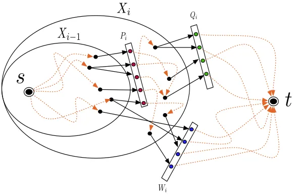
we define the following sets (see Figure2) :
• Yi=Xi\Xi−1
• Pi=Yi∩N+(Xi−1)
• Qi=N+(Xi)\N+(Xi−1)
• Wi =N+(Xi)\Qi
with P1 = {s}. That is, Pi is defined to be those vertices inYi (which is non-empty due to Property 1 in Lemma 4.1) which are out-neighbors of vertices inXi−1, Qi is the set of those vertices in the out-neighborhood of
Xi which arenot in the out-neighborhood ofXi−1and Wiis the set of vertices in the out-neighborhood ofXi which are not already inQi. Observe thatQi can also be written asQi= (V(D)\Xi)∩(N+(Yi)\N+(Xi−1)).
Also note that Pi and Qi are by definition disjoint. Furthermore, it is important to note thatPi andQi are non-empty. The setPi is non-empty because Property 1 of Lemma4.1 guarantees that the setYi is non-empty and Property 2 of Lemma 4.1ensures that every vertex in Xi (and hence in Yi) is reachable from s in D[Xi] implying that there is at least one vertex inYiwhich has a vertex inXi−1 as an in-neighbor. On the other hand,
ifQi is empty thenN+(Xi) =Wi andN+(Xi−1)⊃Wi (strict superset sincePi is non-empty). This contradicts Property 3 of Lemma4.1. Finally, note thatP1={s}, Qq+1={t}, W1=Wq+1=∅ andPq+1=N+(Xq). For each 1≤i≤q+ 1 we define the digraphDias follows:
V(Di) = (Yi\Pi)∪ {si, ti} ∪Wi
A(Di) =A(D)[Yi\Pi]
[
{(si, p)|p∈(N+(Pi)∩(Yi\Pi))∪Wi}
[
{(p, ti)|p∈N−(Qi)∪Wi}
Finally, if Qi∩N+(Pi) 6= ∅, then we add an arc (si, ti). That is, the digraphDi is defined as the digraph obtained fromD[Yi∪Qi] by adding the vertices inWi, identifying the vertices of Pi into a single vertex called
si (removing self-loops and parallel arcs), identifying the vertices ofQi into a single vertex calledti and adding arcs fromsi to all vertices in Wi and from all vertices inWi toti. SincePi andQi are disjoint and non-empty, this digraph is well-defined. Also note that there is no isolated vertex in Di. This is because every vertex in
Di is reachable fromsi by definition. We now make the following claim regarding the connectivity fromsi toti in the digraphDi.
Claim 2. For each1≤i≤q+ 1,λDi(si, ti)> `.
X
iX
i 1 PiQi
Wi
s
[image:14.612.162.453.80.273.2]t
Figure 2: An illustration of the various sets defined in the proof of Lemma4.4. The dotted arrows denote directed paths while the solid ones denote arcs.
The claim above allows us to recursively apply our algorithm to compute tight separator sequences on each graph Di while Claim 2 guarantees a bound on the depth of this recursion. The next claim shows that once we recursively compute a tight separator sequence in each of these digraphs, there is a linear time procedure to combine these sequences to obtain a tight separator sequence in the original graph.
Claim 3. For each1≤i≤q+ 1, letLi denote a tight
si-ti separator sequence {Li1, Li2, . . . , Liri} of order kin
the digraphDi. For each1≤i≤q+ 1and1≤j≤ri,
let Hi
j denote the set(Lij\ {si})∪Pi. Then, the ordered
collection Hdefined asX0∪H11, . . . , X0∪Hr11, X1, X1∪
H2
1, . . . , X1∪Hr22, . . .,Xq, Xq∪H1q+1, . . . , Xq∪Hrqq+1+1 is
a tight s-t separator sequence of orderk inD.
We now use the claims above to complete the proof of the lemma.
Description of the algorithm. We begin by running the algorithm of Lemma4.1on the graphD withsand
t the same as those in the premise of the lemma. If this subroutine concludes that there is nos-tseparator of size at mostkinD then we return the same. Otherwise, the subroutine returns the setsX1, X2\X1, . . . , Xq\Xq−1
corresponding to the collectionX ={X1, . . . , Xq}. We defineXq+1 to be the setR(s,∅)\ {t}.
Having computed the sets X1, . . . , Xq+1, for each
1 ≤ i ≤ q + 1 we compute the graph Di, and
recursively compute the setsLi
1, Li2\Li1, . . . , Liri\L
i ri−1 corresponding to a tightsi-ti separator sequenceLi =
{Li1, Li2, . . . , Lrii} of order k in the graph Di. At this point, we note a subtle computational simplification we use. In order to compute Li, for those Dis where
Wi6=∅, we can invoke Lemma4.3and compute a tight
si-ti separator sequence of orderk− |Wi|in the graph
Di−Wi. As a result, we never actually need to construct the entire graphDias defined earlier. Instead it suffices to constructDi−Wi. The reason behind this is that we can now consider the arcs in the graphs D1, . . . , Dq+1
to be a partition of a subset of the arcs inD.
For each 1 ≤ i ≤ q + 1 and 1 ≤ j ≤ ri, let
Hi
j denote the set (Lij \ {si}) ∪ Pi. We output the sets H1
1, H21 \ H11, . . . , Hr11 \ Hr11−1, X1 \ Hr11−1, H2
1, H22\H12, . . . , Hr22 \Hr22−1,X2\Hr22−1,. . . which
cor-respond (by Claim3) to a tights-t separator sequence
H = H1
1, . . . , Hr11, X1, X1 ∪ H12, . . . , X1 ∪ Hr22, . . .,
Xq, Xq ∪H1q+1, . . . , Xq ∪Hrqq+1+1 or order k. Since the correctness is a direct consequence of Claim 3, we now proceed to the running time analysis.
Running time. We analyse the running time of this algorithm in terms of k, m and λD(s, t). We let
T(k, λ, m) denote the running time of the algorithm whenλ=λD(s, t). If λ > k, thenT(k, λ, m) =O(km). This is because in this case, we only require a single execution of the algorithm of Lemma 4.1 to conclude that k < λ. Otherwise, the description of the algorithm clearly implies the following recurrence.
T(k, λ, m) =O(λm) + q+1 X
i=1
T(k, λi, mi)
whereλi =λDi(si, ti) andmi denotes the number of arcs in Di. Note that m ≥ Pqi=1+1mi. The O(λm) term includes the time required to execute the algorithm of Lemma4.1as well as the time required to compute the graphsD1, . . . , Dq+1. Now, due to Claim2, we have
thatλi> λfor eachi∈[q+ 1]. Unrolling the recurrence with λ > k being the base case, the claimed running time follows. This completes the proof of the lemma.
5 Proving Lemma 1.1
Definition 7. Let D be a strongly connected digraph
and letu, v ∈V(D). LetS ⊆V(D)be au-v separator in D. Then, we say that S is
• anl-good u-v separator ifD[R(u, S)]is acyclic but D[N R(u, S)] contains a cycle.
• an r-good u-v separator if D[R(u, S)] contains a cycle butD[N R(u, S)] is acyclic.
• a dual-good u-v separator if both D[R(u, S)] and D[N R(u, S)] contain cycles.
• acompletely-goodu-v separator ifD[R(u, S)]and D[N R(u, S)] are both acyclic.
• an l-lightu-v separator if |A[R(u, S)]| ≤ 1 2|A(D)|.
• anr-lightu-vseparator if|A[N R(u, S)]| ≤ 12|A(D)|.
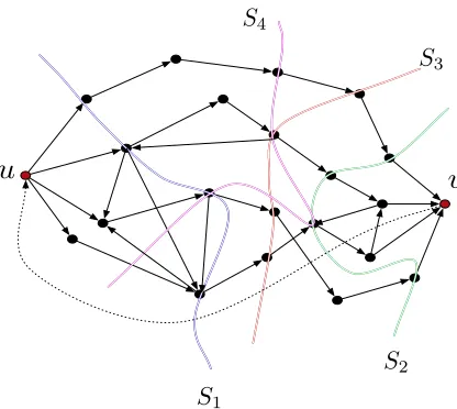
See Figure 3 for an illustration of separators of various types. The next lemma shows that a pair of separators in D with one covering the other have a certain monotonic dependency between them regarding their (l/r)-goodness and (l/r)-lightness.
Lemma 5.1. (Monotonicity Lemma (DFVS)) Let D be a strongly connected digraph. Let u, v∈V(D)and let S1 and S2 be a pair ofu-v separators in D such that S2 coversS1. Furthermore, suppose that neitherS1 nor S2 isdual-good orcompletely-good. Then the following
statements hold.
• If S1 isr-good thenS2 is alsor-good.
• If S2 isl-good thenS1 is also l-good.
• If S1 isr-light then S2 is also r-light.
• If S2 isl-light then S1 is alsol-light.
S
1S
2S
3S
4 [image:15.612.327.535.77.263.2]u
v
Figure 3: An illustration of the various u-v separator types. Here, S1 isl-good, S2 isr-good, S3is dual-good
andS4iscompletely-good.
Proof. We begin by proving the first statement of the lemma. Suppose to the contrary that S1 isr-good and S2isl-good. By definition, the graphD1=D[R(u, S1)]
is not acyclic and D2=D[R(u, S2)] is acyclic. However,
since S2 covers S1, we know thatR(u, S2)⊇R(u, S1).
This implies thatD1is a subgraph ofD2. However, since D1 has a cycle,D2 cannot be acyclic, a contradiction.
This completes the proof of the first statement. The proofs of the remaining statements are all analogous.
We now prove the following lemma which provides a linear time-testable sufficient condition for a separator to reduce the size of the solution upon deletion.
Lemma 5.2. LetDbe a strongly connected digraph. Let u, v ∈V(D),k∈Nand suppose that every dfvs ofD of
size at mostkhits allu-vpaths inD. LetZ be anr-good (l-good) u-v separator of size at mostk such that there is no u-v separator of size at most kcontained entirely in the set R(u, Z) (respectively N R(u, Z)). If D has a dfvs of size at most kdisjoint from {u, v} then D−Z has a dfvs of size at mostk−1.
Proof. LetX be a dfvs ofD. Consider the case whenZ
is anr-good separator. The argument for the other case is analogous. SinceZisr-good, we know that the subgraph
D[N R(u, Z)] is acyclic. Therefore, any non-trivial strongly connected component in the digraph D−Z
lies in the set R(u, Z). Also, the setX0=X∩R(u, Z) is by definition a dfvs of D[R(u, Z)]. Since every non-trivial strongly connected component of D−Z lies in
the digraph D[R(u, Z)], it follows that X0 is in fact a
dfvs forD−Z. We now claim thatX0⊂X.
Suppose to the contrary that X0 = X. By the premise of the lemma, we have thatX is au-vseparator of size at most k. Since X0 =X, we conclude thatX
is au-v separator of size at mostk which is contained in the setR(u, Z), a contradiction to the premise of the lemma, implying thatX0 ⊂X. This completes the proof
of the lemma.
Having set up the definitions and certain properties of the separators we are interested in, we now describe our linear time subroutines that perform certain compu-tations on separator sequences that will then be used in the linear time implementation of our algorithm.
In this lemma, we argue that given the output of Lemma 4.4, one can, in linear time find a pair of consecutive separators in the sequence where the first isl-light and the second one is not. The output of this lemma will form an ‘extremal’ point of interest in the algorithm of Lemma1.1.
Lemma 5.3. LetD be a strongly connected graph. Let u, v∈V(D),k∈N. LetH={H1, . . . , Hq} be a tightu
-v separator sequence of orderk inD with the algorithm of Lemma4.4 returning the setsH1, H2\H1, . . . , Hq\
Hq−1. There is an algorithm that, givenD, u, v, k and
these sets, runs in time O(km) and computes the least i for which the separator N+(H
i) is l-light and the
separator N+(H
i) is not l-light (and consequently is
r-light) or correctly concludes that there is no such
1≤i≤q.
The next lemma provides a linear time subroutine that checks whether the subgraph induced by the set
H2\N+[H1] is acyclic, for a pairH1, H2 of consecutive
sets in the tight separator sequence computed by the algorithm of Lemma4.4.
Lemma 5.4. LetD be a strongly connected digraph. Let u, v∈V(D)andk∈N. LetH={H1, . . . , Hq}be a tight
u-vseparator sequence of orderkinDwith the algorithm of Lemma4.4 returning the setsH1, H2\H1, . . . , Hq\
Hq−1. There is an algorithm that, givenD, u, v, k and
these sets, runs in time O(km)and computes the leasti for which the subgraph D[Hi+1\N+[Hi]]is not acyclic
or correctly concludes that there is no such1≤i≤q−1.
Proof. The proof of this lemma is similar to that of the previous lemma. Given the sets H1, H2\H1, . . . , Hq\
Hq−1 we label the vertices of V(D) in the following
way with elements from{1, . . . , q}. We set H0 ={u}, Hq+1=V(D) and for eachi∈ {0, . . . , q}, we label the
vertices of Hi+1\Hi with the label i+ 1. For each 0≤i≤q, we do a directed bfs/dfs on the set of vertices which are labeledibut not marked as being part of the set N+(H
j) for somej < i. Since each arc is examined
O(k) times, the time bound follows.
Having set up all the required definitions as well as the subroutines tailored to Lemma1.1, we now proceed to its proof.
Lemma 1.1. LetD be a strongly connected digraph and p∈N. There is an algorithm that, given D and p, runs
in time O(p2m) (wheremis the number of arcs in D)
and either correctly concludes thatD has no dfvs of size at mostpor returns a setS with at most 2p+ 2 vertices such that one of the following holds.
• S is a dfvs forD.
• D−S has at least 2 non-trivial strongly connected components (strongly connected components with at least 2 vertices).
• The number of arcs of D whose head and tail occur in the same non-trivial strongly connected component of D−S (arcs participating in a cycle of D−S) is at most m2.
• If D has a dfvs of size at mostpthenD−S has a dfvs of size at most p−1.
Proof. We execute the algorithm of Lemma4.4to either conclude that there is nou-vseparator of size at most
p or compute a tight u-v separator sequence of order
p. If this algorithm concludes that there is no u-v
separator of size at mostpinD, then we return the same. Hence, we may assume that the subroutine returns sets
H1, H2\H1, . . . , Hq\Hq−1 corresponding to a tightu-v
separator sequenceH={H1, . . . , Hq}of orderp. We let Zi denote the setN+(Hi) for each 1≤i≤q and focus our attention on the sets Z1 andZq (which are not necessarily distinct). We begin by examining the setZ1. IfZ1 isdual-good then settingS =Z1 satisfies
Property 2. This is because we started with a strongly connected digraph and by the definition ofdual-goodness both subgraphsD[R(u, Z1)] and D[N R(u, Z1)] contain
cycles and henceD−Z1has at least 2 non-trivial strongly
connected components. Similarly, if Z1 is completely
-good, then setting S = Z1 satisfies Property 1. Now,
suppose thatZ1isr-good. It follows from Definition6
that there is nou-vseparator of size at mostpcontained entirely in the set R(u, Z1). Then, by Lemma 5.2, if D has dfvs of size at mostpdisjoint from {u, v}, then
D−Z1has a dfvs of size at mostp−1 and hence we set S =Z1∪ {u, v}and we satisfy Property 4. Therefore,
going forward, we assume that Z1 is l-good. That is,