Subcontracting and the Survival of Plants in the Road
Construction Industry: A Panel Quantile Regression
Analysis
∗
Dakshina G. De Silva
Lancaster University
Georgia Kosmopoulou
University of Oklahoma
Carlos Lamarche
†University of Kentucky
February 22, 2017
Abstract
This paper investigates how subcontracting parts of contracted work shapes entrants’ success and survival. We find that newly developed quantile regression approaches can be adapted to study survival of firms competing for government contracts in road construction. The method is applied on a data set that includes patterns of firm entry, exit and auction related information. We find an apparent increase in the business life of firms who subcontract out part of their projects. In Texas, these subcontracting effects appear to be more pronounced for firms with few or no options outside the industry, and among firms who contract out part of their work to Disadvantaged Business Enterprises.
JEL Classification: C31, C41, D44, H57, L74.
Keywords: Entrants, procurement auctions, survival analysis, quantile regression.
∗We are grateful to George Deltas, Tim Dunne, Matt Harding, Shakeeb Khan, Roger Koenker, Justin
Marion, and Hisayuki Yoshimoto and participants at the 2nd conference on “Auctions, competition, regula-tion, and public policy” at Lancaster University and the 14th annual International Industrial Organization Conference for comments and suggestions. We are indebted to staff at the Texas Department of Transporta-tion and Texas Workforce Commission for providing useful informaTransporta-tion. The authors obtained these data under an agreement of confidentiality and disclosure of the actual data is subject to certain restrictions. Any opinion, findings, and conclusions or recommendations expressed in this material are those of the authors and do not necessarily reflect the views of the National Science Foundation.
†Dakshina G. De Silva is Professor at Lancaster University Management School, LA1 4YX, UK. Email:
1
Introduction
Subcontracting allows a firm to unbundle contracts and share tasks with a network of business
competitors, thus capitalizing on firm asymmetric strengths. The use of subcontractors
varies across procurement auction settings, and the choices made affect entry and bidding.1
Little is known, however, about the effect of subcontracting on firm survival and whether
it has a differential impact across competitors by their level of market experience. In this paper, we take a closer look at subcontracting and its effect on business duration, offering
an estimation approach that can accommodate double censoring and endogenous covariates,
commonly encountered in the analysis of panel duration data.
The firms we consider in our sample compete for public procurement contracts. The size of the public procurement activity in 2013 reached 13% of the GDP in the United States,
16% in the European Union and 12% across OECD countries, excluding procurement by
state owned utilities.2 Most of these contracts are allocated via simple auction mechanisms.
Theoretical research by Jeitschko and Wolfstetter (2002) and De Silva, Jeitschko and
Kos-mopoulou (2005) points to the fact that potential learning benefits for the winner create
incentives for competitors to engage in risky behavior leading often to a serious bankruptcy
problem (Leufkens, Peeters and Vermeulen (2010)). Under such competitive pressures, firms
could contract out part of their work to ameliorate uncertainty and share information and
expertise. Subcontracting allows bidders to control future costs by smoothing out work-load obligations, leading possibly to a reduction in firms’ information rents (Jeriorski and
Krasnokutskaya, 2016). Transaction costs associated with subcontracting can often put
sig-nificant upward pressure on project costs (Miller, 2014). In an effort to explore ramifications
of the trade-off that exists between the uncertainty involved and the resulting profitability,
we focus on firm survival at early stages of a firm’s development, when entrants are likely
to be inexperienced and uncertain about their costs but can take advantage of
opportuni-ties to subcontract out part of their business activity. We distinguish among firms based
on opportunities for work outside road construction and whether they subcontract their
work to Disadvantaged Business Enterprises (or DBEs) in response largely to policy driven
1
See for example Gil and Marion (2013), Marion (2015), Moretti and Valbonesi (2015), and Branzoli and Decarolis (2015).
2
participation goals.3
This paper proposes a new quantile regression approach for doubly censored data to
investigate the survival of establishments competing for goverment procurement contracts.
Double censoring, or left-censoring and right-censoring, occurs often in the analysis of
pro-curement data because the age of incumbents is not observed at the time of participation in
auctions and information is limited by the length of the observation window. Lack of access
to historical information about a population of interest is an issue in many longitudinal
sur-veys related to unemployment duration, labor markets outcomes studied through recorded histories, educational outcomes and schooling durations. It is often a problem in firm market
survival analysis across all industries and expansion through penetration in foreign markets.
While most of the quantile regression literature focuses on the cross-sectional case, we
pro-pose a flexible semiparametric method for a panel duration quantile regression model with
endogenous covariates. For example, Lin, He and Portnoy (2012), and Ji, Peng, Cheng
and Lai (2012) offer semiparametric approaches for double censored data for cross-sectional
models with exogenous covariates.4 Our methodology is built upon the approaches
consid-ered in Ji, Peng, Cheng and Lai (2012), Harding and Lamarche (2012), and Chernozhukov,
Fern´andez-Val and Kowalski (2015).
We estimate a panel quantile model for establishments’ survival in the market while
controlling for unobserved firm heterogeneity as in Harding and Lamarche (2012). This is
important since subcontracting activities are likely to be endogenous. The quantile approach
is useful in examining the apparent increase in business life of conditionally young firms who subcontract out part of their active projects. We apply the method to a newly-constructed
data set of establishments that allows an empirical investigation of the survival of plants in
road construction. Our main result indicates that utilizing subcontractors that can share
information and part of the uncertainty can have a positive effect on duration in business, in
3
DBEs are defined as small businesses that are owned and controlled by members of a minority group including women-owned businesses and historically underrepresented businesses. Marion (2009, 2015) and De Silva, Dunne, Kosmopoulou, and Lamarche (2012) investigate the potential effects of DBE subcontracting on the cost of procurement contracting.
4
particular at early stages of a firm’s life. The empirical evidence suggests that those effects
seem to be more pronounced for firms with limited business options outside road construction
and those who employ DBE subcontractors. DBE subcontracting is often dictated by policy
aiming to increase representation of underrepresented populations in business. Research has shown that more often than not these policies increase the cost of procurement (Marion 2009).
Our results suggest that the employment of DBEs as subcontractors prolongs business life at
low conditional quantiles, creating externalities significantly larger than those by non DBE
firms. A possible explanation is that, in Texas, a DBE program appears to have encouraged
the formation of a large number of DBE subcontractors who have gained experience in
specific tasks and therefore can help firms to smooth out constraints of contracting.
These findings offer new evidence on the survival of plants in the road construction
industry which is highly concentrated (see De Silva, Kosmopoulou and Lamarche, 2009).
They also suggested that newly enacted programs similar to Mentor-prot´eg´e programs in
Texas and Connect2DOT in Colorado, which have now been adopted in more than thirty
states and provide firms the opportunity to create a network of subcontractors, can enhance
their survival, particularly among entrants who are vital to the competitiveness of the market,
and firms with limited opportunities outside road construction. The results complement the empirical studies analyzing the success of entrants in other manufacturing and service
industries, retailing and agriculture (see Seim (2001), Dunne, Jensen and Roberts (2009),
and Helfat and Lieberman (2002) for a review).
The paper is organized as follows. Section 2 discusses the theoretical model framing our statistical analysis. It also presents the quantile regression model and method. Section 3
describes the data, and it offers the main empirical results. Section 3 also examines the
role of business opportunities outside the state procurement contracts on firm’s survival.
Section 4 has concluding remarks. Finally, Appendix A presents evidence on the small
sample performance of the approach.
2
Survival of Plants: Theory and Estimation
The next section considers a dynamic framework that creates a link between government
de Paula (2010). We focus on subcontracting activity which is widespread and has no
institutional limit per contract. Later in Section 2.2, we propose a panel quantile estimator
for the analysis of the survival of plants in the road construction industry which allows us
to investigate the effect of subcontracting on conditionally low durations.
2.1
Modeling Framework
Firm i (or establishment i, as in the empirical application) is in the construction industry
primarily competing for contracts. The competition determines how long it will continue
being active in business by selecting an optimal continuation strategy that leads to an exit
timeT. The firm also decides whether to subcontract out part of a project. This is motivated by the fact that in our data, which is described in Section 3.1, 87.37% of prime contractors
subcontract out a percentage of the contracted tasks and the number of subcontractors in
government procurement projects ranges from 0 to 35. On average, 20.43% of a contract’s
value is subcontracted out.
Considerπ to be the profit function of a firm consisting of the net payoff from contracting activity, and the payoff from complementary business activity. The profit related to
con-tracting activity, πC, is a function of auction, bidder and rival characteristics x∈ X⊂Rp1,
and the size of firm and involvement in subcontracting activity captured by the vector
s∈S⊂Rp2. In our econometric specification introduced in section 3, p
2 = 2. At any time
t, therefore, the profit function of a representative firm takes the following form
π(x,s, t) =πC(x,s, t) +A(t), (2.1)
where A(t) represents an outside option assumed later to be A = 0 to distinguish firms by their dependence on road construction procurement. We also assume that πC(x,s, t) =
V(x,s, t, θ(x,s))−C(x,s, t, f), where V(x,s, t, θ(x,s)) := W(x,s)θ(x,s)φ(t) is the ex post
value of a contract to a firm, W(x,s) is the payoff related in part to auction and bidders characteristics, and θ(·,·) is a firm specific productivity index that can enhance the profit
from procurement contracting. We assume φ(t) > 0 for t > 1 and φ(0) = 0. The term
C(x,s, f, t) is a cost function related to bidder characteristics, project characteristics, size
and subcontracting opportunities, a fixed operating cost, f, and t. We let C(x,s, f, t) =
with ψ(0) = 0). Finally, we assume, for simplicity, the outside option A(t) =Aψ(t).
Assuming an exponential discount rate ρ, we can express the net profit from road
con-struction business until time t as
Z t
0
πC(x,s, z)e−ρzdz =
Z t
0
[W(x,s)θ(x,s)φ(z)−h(x,s, f)ψ(z)]e−ρzdz. (2.2)
Then the cumulative profit across activities is
Z t
0
[W(x,s)θ(x,s)φ(z)−h(x,s, f)ψ(z)]e−ρzdz+
Z t
0
Aψ(z)e−ρzdz. (2.3)
Conditional on size and subcontracting decisions, optimizing behavior with respect to t
requires that the firm will continue to be in business as long as the benefit of being active
at timet exceeds the cost and the value of the outside option, i.e.,
W(x,s)θ(x,s)φ(T) = (h(x,s, f)−A)ψ(T). (2.4) This first order condition determines the optimal timing T for exit. Conditional on the
optimal timing decision, the firm will choosesto maximize the value of the objective function subject to the constraint that s depends upon w which is defined as a vector of exogenous variables that do not affect a firm’s decision to exit and exogenous restrictions related to
the use of disadvantaged business enterprises as subcontractors based on government set
goals. These variables will serve as instruments in our econometric specification and will be
discussed at length in section 3.2 within the context of our empirical application. Specifically
the objective is to
max
s∈S Π(T(s)) = maxs∈S {W(x,s)Φ(T(s))θ(x,s)−(h(x,s, f)−A)Υ(T(s)) +λ(s−ζ(w))} (2.5)
where λ is a Lagrange multiplier, ζ(·) is a known smooth function, Φ(T) = R0T φ(z)e−ρzdz,
and Υ(T) = R0T ψ(z)e−ρzdz. We shall consider this more general case in section 3.3, although
in what follows, we concentrate on the case of no outside business opportunities by assuming
A= 0.
Letφ(T)/ψ(T) =ξ(T). Under mild conditions, these two optimization problems produce
a system of interdependent equations that can be written as:
T = ξ−1(h(x,s, f)/W(x,s)θ(x,s)) (2.6)
It follows from equation (2.6) that
lnξ(T) = −lnW(x,s)−lnθ(x,s) + lnh(x,s, f). (2.8)
The economic model in (2.8) leads to a simple, yet convenient statistical model that fits
within a class of duration models. For instance, appropriate choices for ξ(T) and W(x,s) lead to the Accelerated Failure Time (AFT) model.5 Following standard practice, we assume
that the ex post value of the contract for a firm is W(x,s) = exp(s′
γ +x′
β). Moreover, we assume that issues associated with possible dependence between a firm’s unobserved
heterogeneity and (x,s) can be addressed by controlling for a duration-invariant omitted variable, α := −lnθ(x,s). Under these assumptions, a version of the model presented in equation (2.8) can be written as
M(T) =s′
γ+x′
β+α+u, (2.9)
where M(·) is a monotone function, in this case the logarithmic function, and u is an error
term distributed as Fu with a conditional variance that depends on x and s. Note that
the error term contains components of the latent cost, and these factors are correlated with
the vector s as in equation (2.7) conditional on individual effects. Lastly, we note that the variable time to exit the market, T, in equation (2.9) is not fully observed as we observe
only,
Y = max{L,min{T, U}}, (2.10)
where the variable Y represents the standard censored response variable, L denotes
left-censoring time, andU denotes right-censoring time. In our application,Lis zero for entrants and the age of the firm for incumbents andU denotes the time period at which we cease to
observe firm activity whether it has exited or not.
Based on this model, we estimate the following quantile regression function:
QM(T)(τ|x,s, α) = s′γ(τ) +x′β(τ) +α(τ), (2.11)
whereQM(T)(τ|x,s, α) = inf{y : Pr(Y < y|x,s, α)≥τ}is theτ-th conditional quantile
func-tion given (s′
,x′
, α) andτ ∈(0,1) is a quantile of the conditional survival times distribution.6
5
See Lancaster (1990), Lee (2008) and Honor´e and de Paula (2010). 6
Quantiles are equivariant to monotone transformations, therefore we can write the previous
model as QM(T)(τ|x,s, α) =M(QT(τ|x,s, α)). Thus, the survival times distribution can be
expressed as QT(τ|x,s, α) = exp{s′γ(τ) +x′β(τ) +α(τ)}.
It is important to emphasize that we concentrate our attention on a quantile version
of equation (2.6) and, as implied by equation (2.7), some elements of the vector s might not be exogenous, even if we condition on firm unobserved heterogeneity, α. For instance,
the size of a new establishment, or subcontracting might not be determined independently
of whether the firm stayed in business as suggested by (2.7). To deal with the potential endogeneity of the independent variables, we adopt the control variable approach proposed
by Chernozhukov, Fern´andez-Val and Kowalski (2015). It basically adds a variable in the
regression so that conditional on it, regressors are not correlated with the error term of the
model. Their approach works in the spirit of Blundell and Powell (2007), although it allows
for a flexible non-additive first stage specification. The control variable is defined as,
v=ψ0(s,x, α,w)≡Fs(s|x, α,w)≡Q
−1
s (s|x, α,w) (2.12) whereψ0(·) is a control function,wis a vector of instruments, Fs is the conditional distribu-tion ofs, andQsis the conditional quantile function ofs. Note thatFsorQscan be estimated by any parametric or semiparametric method. Therefore, P(T ≤ QT(τ|s,x, α)|v,x, α) is
equal to the quantile τ. This assumption is standard in the quantile regression literature
and is equivalent to require that u(τ) =T −QT(τ|s,x, α) has zero τ-th quantile conditional
onv, x, andα.7
2.2
Estimation
To obtain consistent and unbiased estimates of the effect of subcontracting on the
condi-tional duration distribution, it is clear that we need to address issues associated with double
censoring and endogenous independent variables at the same time. This section proposes
quantile function of the response variable while controlling for heterogeneity, sayα. This model can be viewed as a conditional model. There are other conditional models available in the quantile regression literature and we refer the reader to Kim and Yang (2011) for additional discussion on marginal and conditional quantile regression models. Moreover, it is also different than the unconditional quantiles work by Firpo, Fortin, and Lemieux (2009) and Fr¨olich and Melly (2013).
7
It can also be considereds=g(w) +v, whereg(w) may be a non-parametric function, andvis an error
term that is not independent from u. Blundell and Powell (2007) approach is similar to the one proposed
a semiparametric estimation approach for the quantile regression model (2.11) that
encom-passes the control variable in (2.12) and double censoring as in (2.10).
Consider, for simplicity, a sample of n firms observed m times.8 As in Harding and
Lamarche (2012), we find the argument that minimizes a quantile regression objective
func-tion with individual effects. In contrast to existing work however, we augment the model by
a control variable.9 LetX
ij = (s′ij,x ′ ij,z
′ i,vˆ
′ ij)
′
where zi is a vector that indicates firmi, and
Ψ(τk) = (γ(τk)′, β(τk)′, α(τk)′, λ(τk)′)′. The estimator of the control variable (2.12) is based
on vij =Q−V1(sij −g(xij,zi,wij)) where g(·) is a known linear parametric function and the
control variable vij can be estimated by the empirical cumulative distribution function of
the least squares residuals.10 Our estimator for Ψ(τ) is then defined as follows:
ˆ
Ψ(τ) = arg min Ψ∈Θ
n X i=1 m X j=1
(log(Yij)−X′ijΨ(τ))(ϑij(τ)−δijI(log(Yij)−X′ijΨ(τ)<0)) (2.13)
where δij equals 1 if Lij ≤Tij ≤Uij and 0 otherwise and,
ϑij(τ) =
q−1 X
k=0
I(Yij ≥exp(X′ijΨ(τk))> Lij)(H(τk+1)−H(τk)), (2.14)
The solution of (2.13),Ψˆ(τ), is called theτ-th panel quantile regression estimator for doubly censored data (PQDC). Naturally, in the case of censored data and exogenous covariates,
one can estimate the model by solving (2.13) while replacingXij by (s′ij,x ′ ij,z
′ i)
′. We employ
this estimator in Section 3.2 and we compare the results with the results obtained by the
PQDC estimator, ˆΨ(τ).
The standard error ofΨˆ(τ) in the next Section 3 is obtained by the bootstrap procedure proposed by Jin, Ying and Wei (2001) and investigated in Ma and Kosorok (2005). This
procedure works under fairly general conditions and can accommodate within block
corre-8
The estimation approach proposed in this section can be naturally applied to different datasets including
balanced and unbalanced panels. In Section 3.2, we estimate the quantile model using m firms with nj
establishments. The implication is that the number of establishments of firm j can be different than the
number of establishments of firmk.
9
WhenLij = 0 for all (i, j) and instruments are used instead of control variables, our proposed estimator is identical to Harding and Lamarche’s (2012) estimator. While an instrumental variable approach to panel duration quantile models with a large number of firms may be regarded by applied researchers as compu-tationally demanding, the approach proposed in this paper solves a relatively simpler linear programming problem that performs extremely well in large size applications.
10
lation.11 Because it maintains the endogenous structure of the model, it can be extended
to include the use of a control function to address the potential endogeneity of size and
subcontracting activities.
3
Survival of firms in the construction industry
In this section, we use a sample of entrants and incumbents to study how procurement
auc-tions shape the survival of firms in the road construction industry. We first perform, in
Appendix A, a brief simulation study to investigate the performance of the proposed
esti-mator. We then employ the estimation procedure developed in this paper and report the
results in Section 3.2. Finally, we perform a series of robustness checks, considering
alterna-tive samples and approaches. Our main results highlight the impact that subcontracting out
can have on duration in business. The proposed approach which has excellent finite sample properties as shown in Appendix A is useful in uncovering the increase in the conditional
business life of young entrants who engage in subcontracting.
3.1
A Description of the data
Our firm-level data were obtained from two sources: the Texas Department of Transportation
(TxDOT) and the Texas Workforce Commission. The data that contain information on bidding activity for highway construction contracts were obtained from TxDOT. They span
the period between July 1999 and December 2006. All projects are auctioned off using a
first-price sealed-bid format. The data set contains information on project types, the engineer’s
cost estimate for each project, the number of bidders that requested plans, the number of
bids submitted per project, the winning bidders, and the winning bids. It also contains the
location and complexity of each project and the number of days until its completion. A
detailed description of the initial information that was collected and the variables that were
subsequently constructed are in Table B.1 in Appendix B. The data set also provides the names of subcontractors for the winning bidders and corresponding negotiated subcontractor
11
Jin, Ying and Wei (2001) and Ma and Kosorok (2005) suggest drawing independent variables from a non-negative distribution with mean 1 and variance 1 (i.e., exponential or Gamma distribution) to perturb
the objective function. In our application, we obtainΨ∗ as the argument that minimizes a perturbed (2.13).
We reiterate this procedureB times to obtain a large sample of realizations{Ψ∗
b} B
b=1. For a given quantile, we can obtain the variance ofΨˆ(τ) by the sample variance of{Ψ∗
Variable All firms Incumbents Entrants Number of firms that held plans 993 629 364
Number of establishments (branches) 1275 751 524
Total number of bids 6,998 5,727 1,271
[7.05] [9.10] [3.49]
Total number of wins 1,668 1,375 293
[1.68] [2.19] [0.80] Number of firms that submit at least a bid 540 394 146
[0.54] [0.63] [0.40] Number of firms that at least won once 341 267 74
[0.34] [0.42] [0.20]
Relative bid 1.077 1.079 1.069
(0.249) (0.247) (0.259)
Relative winning bid 0.970 0.974 0.946
(0.177) (0.176) (0.181)
Number of employees 75.935 70.110 92.567
(247.727) (198.236) (265.410) Number of months in the market 51.579 64.855 32.553
[image:11.595.106.519.106.414.2](35.577) (34.383) (27.788)
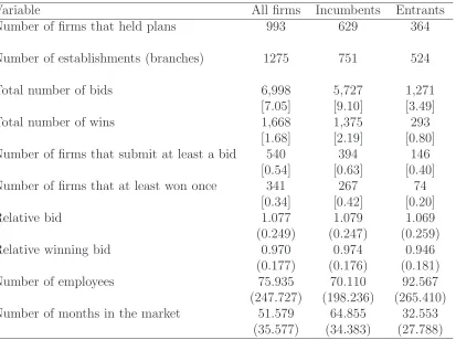
Table 1: Descriptive statistics for the TXDOT-QCEW data. The sample includes existing firms (Incumbents) and new firms that entered the market in the period July 1999-December 2006 (Entrants). Relative Bid is defined as bid divided by the engineer’s cost estimate and Relative winning bid as winning bid divided by the engineer’s cost estimate. Statistics scaled by the number of firms are shown in brackets and standard deviations are in parentheses.
dollar values. This allows us to identify primary bidders who have initially participated as subcontractors in TxDOT auctions.
Establishment-level monthly employment and quarterly wage data for Texas
establish-ments were obtained from the Texas Workforce Commission’s Quarterly Census of
Employ-ment and Wages (QCEW) data base. This data base, as required under the Texas unem-ployment insurance (UI) program, provides establishment-specific monthly emunem-ployment and
quarterly total wages. It also includes each firm’s business start-up date, the specific loca-tion of the establishment, and the six-digit North American Industry Classificaloca-tion System
(NAICS) code. Separate establishments (branches or plants) of the same firm are identified
and reported in separate records. This allows us to identify firm level expansions or
1999 2001 2003 2005
Entry Year
Number of Entrants
0
10
20
30
40
50
60
Ever Plan Holders Ever Bidders Ever Winners
[image:12.595.134.460.143.342.2]1999 2001 2003 2005
Exit Year | Entry
Number of Entrants
0
10
20
30
40
50
60
Ever Plan Holders Ever Bidders Ever Winners
Figure 1: Frequencies for the number of entrants and exitors. The x-axis on the left panel
considers the year of entry for entrants after July 1999. The x-axis on the right panel
considers the year of exit for firms that entered the market after July 1st, 1999. The shaded areas denote firms’ activities related to the procurement auctions.
or temporary expansions (contractions) could be due to the natural rate of firm growth (de-clines) or to absorption of a temporary shock due to winning (completion of) a long term
project in a distant location from the main office. The appearance of a new Employer
Iden-tification Number (EIN) and firm start-up date signifies entry and disappearance of an EIN
record signifies exit. This is similar to the definition used by Baldwin and Gorecki (1991) and
Dunne, Roberts and Samuelson (1988)).12 In a similar way, we also use the establishment
start date and employment patterns to identify entry and exit. However, our data suggest
that bids are generated from the main office and not from branches.
Table 1 reports information on all firms that held plans (plan holders) during this
pe-riod.13 A unique characteristic of this market is that there are a large number of plan
12
The data allows us to identify changes in the names of firms. Those changes should not be counted as exit (Dunne et al. 1988). Moreover, we can identify horizontal mergers.
13
0 2 4 6 8 10 12 14
0.0
0.2
0.4
0.6
0.8
1.0
Single establishment
Subcontractors in Active Projects
0 2 4 6 8 10 12 14
0.0
0.2
0.4
0.6
0.8
1.0
Single establishment
DBE Subcontractors in Active Projects
0 2 4 6 8 10 12 14
0.0
0.2
0.4
0.6
0.8
1.0
Multiple establishments
Subcontractors in Active Projects
0 2 4 6 8 10 12 14
0.0
0.2
0.4
0.6
0.8
1.0
Multiple establishments
[image:13.595.134.486.198.566.2]DBE Subcontractors in Active Projects
holders that are capable of intensifying competitive pressures intermittently through the
bidding process. There are 993 different plan holders and 540 bidders in this data set. Table
1 also provides information on relative bids and relative winning bids which are bids that
are normalized by their engineering cost estimates. The average relative bid is 1.077 and the average relative winning bid is 0.970. These incumbent firms had about 70 employees per
branch and on average, survived about 64 month. Column 3 reports the summary statistics
for entrants. Entrants are bidding lower and are winning with more aggressive bids. We
observe that there are 364 entrants and 74 of them are contractors in the period of analysis.
They stay in the market for about half of the life of incumbents.
The sample of entrants include 214 plan holders and 41 firms (with potentially many
branches) that won a project at least once in their early stages. Using this sample of
entrants, Figure 1 shows the empirical distributions of firms’ entry and exit. Note that these
estimates do not suffer from biases arising from left-censoring. The first panel presents the
number of plan holders that enter the market. Approximately 41 percent of firms became
bidders and 20 percent became winners in the period of analysis. We see that the number
of firms entering the market increased in the period 1999-2001, and had a decreasing trend
after 2001. Nevertheless, the year of entry does not seem to be a critical determinant of the probability of winning. While 20 percent became contractors in the period 1999-2001, 19
percent became contractors in the period after. The second panel presents the number of
plan holders that exited the market in the same period of analysis. The evidence indicates
that no firm that entered the market in either 1999 or 2000 exited the market in those years.
As illustrated in Figure 2, there are high- and low-subcontracting establishments and the
number of subcontractors in active projects depends on the number of branches per firm. The
total number of subcontractors ranges from 0 to 35, with a mean of 1.86 subcontractors in
active projects.14 To make Figure 2 clearer, we limit the number of subcontractors in active
projects to 14. The panels also shows that high-subcontractor establishments are typically
part of a firm with multiple establishments. When we focus on Disadvantaged Business
Enterprises, the number of DBE subcontractors is naturally smaller. Nevertheless, 2555
14
0 10 20 30 40 50 60 70
−1.5
−1.0
−0.5
0.0
0.5
1.0
1.5
2.0
Survival time
Log of relative employment
Individual Contractor
cs: First time contractor who subcontracts c: First time contractor
e: Market exit cs
c
e
0 10 20 30 40 50 60 70
−1.5
−1.0
−0.5
0.0
0.5
1.0
1.5
2.0
Survival time
Log of relative employment
a: Contractor wins first asphalt project b: Contractor wins first bridge project e: Market exit
e b
[image:15.595.123.473.141.407.2]a Individual Contractor
Figure 3: Profile of contractors’ relative size. They-axis shows the logarithm of employment relative to initial employment and the x-axis the number of months from establishment in business. The letters cs and c indicate events in the firms’ life related to the procurement auctions: cs denotes first time contractor who subcontract out part of the project, and c indicates first win as primary contractor who does not subcontract out part of the project. The letters a indicates asphalt, b denotes bridge, and e denotes exit time.
projects have some DBE goals. Such goals are set on federal projects only. The average DBE
goal is 3.40 of the contracted value across all federal projects and 6.31 across all projects with
actual DBE goals. It is interesting to see that more than 90 percent of single-establishment
firms, which are typically entrant firms, do not use DBE subcontracting.
A graph on business activity of individual contractors can provide intuition about the
role of procurement auctions on firm survival. Figure 3 considers four contractors and offers
a cursory look at employment patterns as a function of time. These firms were selected
for their value in emphasizing activities and survival paths that later prove to be quite
business. The longitudinal dimension of the data tentatively ascribes the apparent influence
of subcontracting out part of the first contract on business duration. Although the firms won
their first projects at a similar age, only the company that subcontracted part of its project
(indicated by the letters cs) seems to have grown over time. The right panel in Figure 3 focuses on relative risks associated with involvement in different type of projects. As seen
on the graph, the contractor who did asphalt work had a steady employment growth despite
the fact that contracting activity for TxDOT started only after the first four and a half
years in business. The size of the entrant in bridge work increased until the first project was
won (indicated by the letter b). Immediately after that, the size of the company decreased
leading eventually to market exit (denoted by e). For this firm survival in business may have
been associated with uncertainty induced by the projects undertaken and lack of outside
business options that can affect the timing of the first win.
3.2
Main Empirical Results
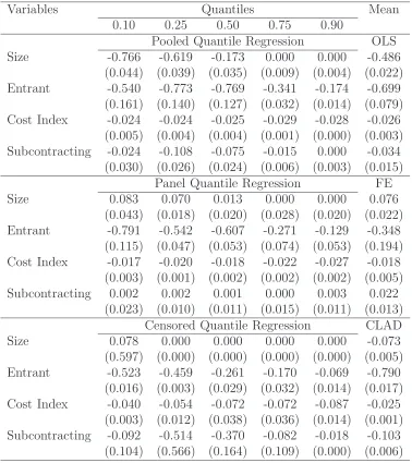
We begin estimating a model for survival times using standard approaches. The results are
shown in Table 2. The dependent variable is duration in the market for an establishment
and the main independent variables are average number of employees (size) of the plant
during the duration of the spell, a binary variable indicating whether the establishment is an
entrant, the cost index of active projects, and the average number of subcontractors that a
firm seeks out. In all the models estimated in this section, we include capacity utilization and backlog variables. The cost index is based on a composite indicator that covers the unit costs
of excavation, resurfacing and construction. It mainly reflects exogenous cost changes for
materials needed to complete highway projects. The table shows quantile regression results,
the fixed effects quantile regression estimator as in Koenker (2004), and quantile regression
results for a model with censored data as in Peng and Huang (2008). We also show results
obtained by Powell’s (1984) CLAD estimator which is designed to address right censoring in
a cross-sectional model with exogenous variables. For completeness, the table shows classical
OLS and fixed effects results. The interested reader can find additional details on how the variables were constructed in Appendix B.
One might argue about the validity of the results presented in Table 2. Several issues
Variables Quantiles Mean 0.10 0.25 0.50 0.75 0.90
Pooled Quantile Regression OLS Size -0.766 -0.619 -0.173 0.000 0.000 -0.486
(0.044) (0.039) (0.035) (0.009) (0.004) (0.022) Entrant -0.540 -0.773 -0.769 -0.341 -0.174 -0.699
(0.161) (0.140) (0.127) (0.032) (0.014) (0.079) Cost Index -0.024 -0.024 -0.025 -0.029 -0.028 -0.026
(0.005) (0.004) (0.004) (0.001) (0.000) (0.003) Subcontracting -0.024 -0.108 -0.075 -0.015 0.000 -0.034
(0.030) (0.026) (0.024) (0.006) (0.003) (0.015) Panel Quantile Regression FE Size 0.083 0.070 0.013 0.000 0.000 0.076
(0.043) (0.018) (0.020) (0.028) (0.020) (0.022) Entrant -0.791 -0.542 -0.607 -0.271 -0.129 -0.348
(0.115) (0.047) (0.053) (0.074) (0.053) (0.194) Cost Index -0.017 -0.020 -0.018 -0.022 -0.027 -0.018
(0.003) (0.001) (0.002) (0.002) (0.002) (0.005) Subcontracting 0.002 0.002 0.001 0.000 0.003 0.022
(0.023) (0.010) (0.011) (0.015) (0.011) (0.013) Censored Quantile Regression CLAD Size 0.078 0.000 0.000 0.000 0.000 -0.073 (0.597) (0.000) (0.000) (0.000) (0.000) (0.005) Entrant -0.523 -0.459 -0.261 -0.170 -0.069 -0.790
(0.016) (0.003) (0.029) (0.032) (0.014) (0.017) Cost Index -0.040 -0.054 -0.072 -0.072 -0.087 -0.025
(0.003) (0.012) (0.038) (0.036) (0.014) (0.001) Subcontracting -0.092 -0.514 -0.370 -0.082 -0.018 -0.103
[image:17.595.117.495.166.591.2](0.104) (0.566) (0.164) (0.109) (0.000) (0.006)
do not have information on whether or not the plant or firm participated in an auction
before the window of observation; (ii) the dependent variable is likely to be right-censored
for entrants and incumbents; (iii) following our framework in Section 2, the variables size and
subcontracting are likely to be endogenous because duration in the market affects size and subcontracting experience of the firm and size or subcontracting are likely to affect duration;
(iv) the independent variables are likely to be correlated with firm latent heterogeneity. None
of the methods employed in Table 2 jointly address these potential issues. It is immediately
apparent that these estimation issues are present in the results associated with size and
subcontracting. In the censored regressions, subcontracting, if anything, has a negative
effect on duration in the market. We also find that size has no effect on survival which
contradicts the existing literature. As we see below, these findings change dramatically
when we address the estimation challenges.
We therefore turn to the estimation of a panel duration model with double censored
data and endogenous covariates. We estimate Tij = exp{s′ijγ + x ′
ijβ +αj +uij}, where Tij denotes the duration in the market in months of plant i associated with firm j. Note
that Tij is latent and we use the observed duration Yij. The variable Lij is equal to zero
for entrants and it is equal to the age of the initial establishment for incumbents. Left censoring occurs for incumbents because we do not observe entry of a branch before 1999.
The variable αj captures effects that are common to establishments within firms.15 In this
model, it seems natural to consider that the size of an establishment s1,ij, measured by the
logarithm of average employment, and subcontractings2,ij, measured by the average number
of subcontractors in active projects, are endogenous.
To address the potential endogeneity of these variables, we generate a control variable
using least squares residuals. Specifically, we obtain ˆvk,ij = Φ−1(sk,ij−R′k,ijπˆ) whereRk,ij =
(wk,ij,x′ij,z ′ i)
′
, xij is a vector of exogenous variables that includes an indicator variable
for whether the establishment is an entrant, a composite variable that cover unit costs of
15
different tasks, capacity utilization and backlog variables,zi is a vector of indicator variables
for the individual effects,k ∈ {0,1}and Φ(·) is the Normal cumulative distribution function.
The “excluded” exogenous variables wij includes the annual change in the number of single
family units approved by building permits prior to the firm’s year of birth and the number of plan holders in active projects. The number of single family units by building permits before
a plant enters the market should be naturally correlated with the number of subcontractors.
On the other hand, pre-determined changes in home renovations including electrical work
and plumbing should be independent of project costs of a plant that participates in the
procurement auctions years later. Moreover, the number of plan holders is uncorrelated
with latent time-varying drivers of survival in the market as the number of plan holders in
an auction identifies the maximum number of bidders that expressed interest in the project
and may submit bids. With respect to the correlation between number of plan holders and size, we argue that the number of plans held by a firm determines the likelihood of winning
and eventually the number of employees needed to complete the project. The number of
plan holders has been used in the empirical auction literature (De Silva, Dunne, Kankanamge
and Kosmopoulou 2008). The other independent variables are considered to be exogenous
variables conditioning on αj. As in Section 2.2, the estimator is obtained in a second step
using the control variable ˆvij.16
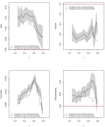
The results are presented in Figure 4. The figure presents estimates of the main covariate
effects as a function of the quantile τ of the conditional distribution of duration. In each
graph, the continuous line shows the point estimates and the shaded region represents a
90% confidence interval for the point estimates. For instance, the first graph on the top row
shows estimates of the effect of size on duration. The estimate is positive and significant
at the 0.25 quantile and it tends to decrease as we go across quantiles. The advantage of
the figure is that it allows us to carefully examine the effect of the independent variables of
interest at any quantile. As expected, the size of the plant is likely to affect the duration in the market which was not implied by the results presented in Table 2. The main results
sug-gest that duration in construction business is affected by the procurement auctions through
subcontracting and changes in the input prices of active projects. (The sole exception is
the effect of subcontracting at the upper tail of the conditional distribution). Having a
net-16
0.2 0.4 0.6 0.8
0.00
0.05
0.10
0.15
0.20
τ
Siz
e
Exogenous Size and Subcontracting Endogenous Size and Subcontracting
0.2 0.4 0.6 0.8
−0.8
−0.6
−0.4
−0.2
0.0
τ
Entr
ant
Exogenous Size and Subcontracting Endogenous Size and Subcontracting
0.2 0.4 0.6 0.8
−0.020
−0.015
−0.010
τ
Cost Inde
x
Exogenous Size and Subcontracting Endogenous Size and Subcontracting
0.2 0.4 0.6 0.8
0.00
0.05
0.10
τ
Subcontr
acting
[image:20.595.119.480.167.604.2]Exogenous Size and Subcontracting Endogenous Size and Subcontracting
0.2 0.4 0.6 0.8
0.00
0.05
0.10
0.15
0.20
τ
Siz
e
Exogenous Size and Subcontracting Endogenous Size and Subcontracting
0.2 0.4 0.6 0.8
−0.1
0.0
0.1
0.2
0.3
τ
DBE Subcontr
acting
[image:21.595.121.476.273.510.2]Exogenous Size and Subcontracting Endogenous Size and Subcontracting
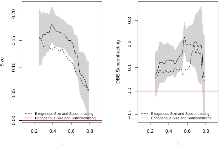
Figure 5: Quantile regression results for the effect of size and subcontracting on duration.
The quantiles of the conditional duration distribution are denoted by τ. The continuous
work of subcontractors that can share information and project risks increases the duration
in business.
We implemented Wald-type tests to evaluate whether the effects of size and
subcontract-ing are different across quantiles. We evaluated whether the effects of interest are significantly
different between two quantiles, say τ1 and τj for j ∈ {2,3, ...M}. The results indicate that
the effect of size is significantly different between the 0.25 and 0.75 quantiles and the effect
of subcontracting is significantly different between the 0.25 and 0.65 quantiles. In the case
of subcontracting, the null hypothesis γ2(0.25) =γ2(0.65) is weakly rejected at 10%.
More-over, to examine the effect of ignoring endogeneity in panel duration models, we offer results
obtained by the same procedure while assuming that size and subcontracting are exogenous.
As explained in Section 2, the estimation procedure is similar but we do not augment the
design matrix with the control variables. As in the case of endogenous variables, the (dashed)
line shows the point estimates.17 The new results suggest that the effect of size is
under-estimated at the low conditional quantiles of the duration distribution if we assume that
size and subcontracting are exogenous. Moreover, the effect of subcontracting is attenuated
towards zero. These results might be interpreted within the framework developed in Section
2.1, which implies that there are latent components of cost not adequately controlled for by other covariates in the τ-th conditional quantile model. Because higher costs are likely to
negatively affect duration, the comparison between point estimates in Figure 4 suggest that
firm cost is increasing in size and number of subcontractors, as one might have expected.18
Figure 5 shows results from estimating the model as in Figure 4 with the exception that subcontracting s2,ij is now measured by the average number of Disadvantaged Business
Enterprises (DBEs) in active projects. To address the potential endogeneity of the DBE
subcontracting variable, we generate the control variables using least squares residuals and
17
Because they to not represent the main findings and to simplify the visual analysis of the results, we do not provide a 90% point-wise confidence interval in Figure 4 for the case of exogenous size and subcontracting. Size remain to be significant atτ≤0.7 but subcontracting is in general insignificant at 10% (the sole exceptions are the estimates around the median conditional quantile).
18
0.2 0.4 0.6 0.8
−0.5
0.0
0.5
1.0
1.5
2.0
τ
Subcontr
acting
At least 1 sub At least 4 subs
0.2 0.4 0.6 0.8
−0.5
0.0
0.5
1.0
1.5
2.0
τ
DBE Subcontr
acting
[image:23.595.119.476.143.380.2]At least 1 sub At least 4 subs
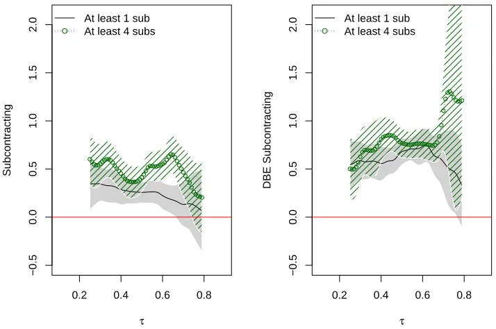
Figure 6: Quantile regression results for the effect of the number of subcontractors on dura-tion. The shaded regions represent a 90 percent point-wise confidence interval.
the same instruments used to obtain the results shown in Figure 4. The excluded exogenous
variables are the change in the number of single family units approved by building permits
prior to the firm’s year of birth and the number of plan holders in active projects, which not
likely to affect duration conditional on firm heterogeneity.19
The findings suggest that when contractors employ as subcontractors minority and women
owned businesses, known as DBEs, the effects on survival are more pronounced.
Addition-ally, we find that the effect of DBE subcontracting appears to be larger among firms using
4 or more DBE subcontractors in the period of analysis (Figure 6). Contrary to what one
would expect, as DBE subcontracting is often linked to government imposed goals that can
lead to inefficiencies (see Marion 2009), Figure 5 suggests that if a relatively young firm has
utilized DBE subcontractors it is likely to survive longer in business. Although the shape of
19
the subcontracting effects is similar to the results shown in Figure 4, the estimated effects
are roughly two times larger at several quantiles including τ = 0.25.20 Even though there
is a large number of minority-owned construction firms in Texas and the program that
en-couraged the formation and success of DBEs has increased the supply of those firms without increasing the cost to the state (see De Silva, Dunne, Kosmopoulou and Lamarche 2012),
the results go a step further to suggest that DBE subcontracting may have positive external
effects on competitors.
Subcontracting allows establishments to smooth out constraints in contracting and there-fore benefits an establishment if other firms have extensive experience in specific tasks. DBE
subcontractors will likely fit this profile because the program in Texas appears to have
encouraged the formation of minority and women owned businesses who often undertake
subcontracting work either within or outside the federally imposed DBE subcontracting
goals.21
There is a long debate on the value of policies targeting small or disadvantaged businesses
with evidence provided on costs and benefits (see Marion (2009, 2015) and De Silva, Dunne,
Kosmopoulou, and Lamarche (2012) for some related findings). Nakabayashi (2013) considers
in a counterfactual estimation the impact on firm exit, of eliminating incentives targeting
small businesses in Japan. He finds that elimination of such programs would induce exit of
40% of existing small business firms. That reduction in competition would increase the cost
of procurement.
3.3
Empirical Evidence from a Sample of Entrants
This section considers a series of robustness checks on the specifications and assumptions
behind the models estimated in the previous section. The results are shown in Table 3.
20
We accommodated existing Wald-type tests to evaluate whether the effects of size and subcontracting in Figure 5 are significantly different across quantiles. The results indicated that the effect of size is not significantly different at 5 percent significance level across quantiles with the exception when we tested the null hypothesis γ1(0.25) = γ1(0.75). The test had a p-value equal to 0.032. Moreover, the effect of DBE subcontracting does not significantly change across quantiles. However, as it can be seen in Figure 5, the effect of DBE subcontracting is statistically significantly different from zero (the exceptions are the lower and upper quantiles of the conditional duration distribution).
21
Sample Effect of subcontracting in active projects Quantiles
0.1 0.25 0.5 0.75 0.9
Entrants 0.715 0.696 0.290 0.148 0.104
(0.314) (0.236) (0.171) (0.062) (0.039) Entrant firms (cohorts 2000 and 2001) 0.283 0.535 0.529 0.167 0.125
(0.354) (0.431) (0.280) (0.136) (0.036) Contractors (cohorts 2000 and 2001) 0.974 0.929 0.626 0.172 0.137
(0.449) (0.340) (0.298) (0.189) (0.061) Entrants firms with outside options 0.584 0.462 0.265 0.161 0.109
(0.376) (0.277) (0.233) (0.088) (0.055) Entrants firms without outside options 0.856 0.806 0.223 0.071 0.029
(0.321) (0.283) (0.193) (0.107) (0.069)
Control variables Yes Yes Yes Yes Yes
Project specific controls Yes Yes Yes Yes Yes
Firm Effects Yes Yes Yes Yes Yes
[image:25.595.76.530.114.357.2]Control function Yes Yes Yes Yes Yes
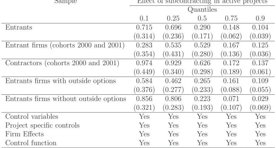
Table 3: Panel duration quantile regression results for the logarithm of survival times. Con-trol variables include size, unemployment and cost index of active projects. Project specific controls include the value of the engineer’s cost estimate of the project, the total number of bid items in a project, and indicators for projects grouped into asphalt and bridge categories. The control variable function is based on the number of plan holders in active projects, a lagged value of the number of plan holders, a lagged value of logarithm of employment and lagged values of number of firms in single-family and multifamily housing construction. The standard errors are obtained after 1000 panel bootstrap repetitions.
These results are obtained by restricting the sample of firms to include entrants and defining
the dependent variable asTij, wherei denotes establishments andj indicates age of the
es-tablishment in months. A survival model forTij can be estimated by the proposed approach,
provided that the data is organized following a m-line record.22 In what follows, we discuss
the importance of subcontracting among entrants, business cycle effects and the effect of work outside the procurement auctions on firms’ duration in business.
22
It refers to the idea that we can split the observed duration data into segments. Duringm−1 periods,
3.3.1 Subcontracting and Survival of Entrants
Following the framework adopted in section 2, as before, we assume that the size of a
firm, measured by the logarithm of total employment, and subcontracting are endogenous
variables. However the difference with respect to our previous results is that we concentrate on the effects of subcontracting using a sample of entrants. To obtain the control variable
function, we include in w the number of plan holders in active projects, a lagged value of the number of plan holders, a lagged value of the logarithm of employment and lagged
values of number of firms in single-family and multi-family housing construction. In addition
to the controls used in the previous section, the model includes project specific covariates
and individual effects, which could be associated to firm specific productivity or level of
involvement in complementary activity that can affect business profit. Notice that these
latent factors may be expected to be correlated with size and subcontracting. Project specific
controls include the value of the engineer’s cost estimate of the project, the total number of
project components in a project, and indicators for projects grouped into the asphalt and bridge categories. The first row of the table shows that the effect of subcontracting in active
projects is positive and significant at the lowest quantiles, suggesting that subcontracting
prolongs (conditional) duration in business. Subcontracting allows one to share valuable
information to reduce uncertainty and risks, and seems to be more important at early stages
of a firm’s life.
3.3.2 Business cycle effects
Price fluctuations related to the business cycle may affect entry in the procurement auctions.
One would think that high oil prices in the 2000’s may have led to entry of relatively
highly-efficient firms. Or alternatively, funds on infrastructure projects to stimulate the economy
simultaneously affected the type of firms buying plans and bidding.23 In order to isolate the
effect of business cycle movements on duration in business, we restrict our sample to include (a) entrants who bought a plan in 2000 and 2001 but did not necessarily win a contract, and
23
(b) firms who did road construction (surfacing/resurfacing) work. Considering these samples,
we re-estimate the models and present the results in Table 3. The evidence is consistent
with the theory and the previous results. It continues to suggest that subcontracting affects
survival of contractors in the road construction industry.
3.3.3 Limited business opportunities outside road construction
The potential losses associated with uncertainty and project risks may be mitigated by
the existence of alternative business options. In light of the framework in Section 2 and theoretical and experimental evidence in Kirchkamp, Poen, and Reiß (2009), it is of interest
to revisit our findings and distinguish among firms by their dependence on road construction
procurement, and consequently, their access to outside business options.24
After discussions with state highway and civil engineers and based on the original NAICS classification and additional information obtained from descriptions of their activities, we
created two relevant groups, and accordingly, in Table 3, we divided the sample of contractors
into two sub-samples: firms with outside options (e.g., landscaping, plumbing, heating,
etc.) and firms with few or no outside options (e.g., bridge construction, highway and
street construction, etc.).25,26 Notice that the first group includes firms whose survival in the
industry does not crucially depend upon the outcome of the procurement auction process for
road construction, and the second group include firms whose survival mainly depends upon
these contracts.
The evidence in Table 3 for firms whose survival does not depend on the procured
gov-ernment projects suggests a positive but insignificant effect of subcontracting at the lowest
quantiles of the survival distribution. While the estimated effect of subcontracting is
insignif-icant at the 0.1 quantile among firms with outside options, it is positive and signifinsignif-icant for
24
Kirchkamp, Poen, and Reiß (2009) studied the effect of the presence of outside options in bidding. They showed that, bidders respond to outside options by softening bidding aggressiveness.
25
The North American industry classification system (NAICS) allows us to distinguish among commercial and institutional building contractors, electrical contractors, highway, street and bridge contractors, firms offering landscaping services, new single-family housing contractors, and other building finishing contractors.
26
firms with few or no outside options. We interpret this result as suggesting that
subcontract-ing can have a more advantageous effect on survival for firms with few or no outside options
(e.g., bridge contractors). It should be noted however that these effects do not appear to be
significantly different at standard levels of significance.
4
Conclusion
This paper investigates how subcontracting parts of contracted work affects firm’s survival.
We apply a panel duration quantile regression approach to a sample of data from firms in road
construction. This industry displays market concentration featuring only a small number of
firms, thus limiting the competitiveness of market outcomes. We construct a unique data
set of entrants and propose a semi-parametric approach that simultaneously addresses issues
associated with firm’s latent heterogeneity, endogenous time-varying covariates and double censored data. The approach offered in this paper appears to perform well relative to other
approaches being studied in the literature of quantile regression for duration data. Our
quantile regression approach allows us to investigate survival beyond the mean effect, which
is important in the context of understanding the determinants of young firms’ duration in
business and the effect of DBE policies on firm survival.
Our results indicate that employing subcontractors can have a positive effect on duration
in business, in particular at early stages of a firm’s life. Those effects are more distinct for
firms with limited business options outside road construction and those who employ DBE
firms as subcontractors. The results also suggest that programs similar to Mentor-prot´eg´e
in Texas and Connect2DOT in Colorado, which provide firms the opportunity to create a
network of subcontractors, can enhance their survival.
References
Baldwin, J. R., and P. K. Gorecki (1991): “Firm Entry and Exit in the Canadian
Manufacturing Sector, 1970-1982,” The Canadian Journal of Economics, 24, 300–323.
Blundell, R., and J. L. Powell(2007): “Censored Regression Quantiles with
Branzoli, N., and F. Decarolis (2015): “Entry and Subcontracting in Public
Procure-ment Auctions,” Management Science, forthcoming.
Cameron, A. C., and P. K. Trivedi(2005): Microeconometrics: Methods and
Applica-tions. Cambridge.
Chen, S.,andS. Khan(2001): “Semiparametric Estimation of a Partially Linear Censored
Regression Model,” Econometric Theory, 17, 567–590.
Chernozhukov, V., I. Fernndez-Val, and A. E. Kowalski(2015): “Quantile
regres-sion with censoring and endogeneity,” Journal of Econometrics, 186(1), 201 – 221.
De Silva, D. G., T. Dunne, A. Kankanamge, and G. Kosmopoulou (2008): “The
Impact of Public Information on Bidding in Highway Procurement Auctions,” European Economic Review, 23(3-4), 150–181.
De Silva, D. G., T. Dunne, G. Kosmopoulou,and C. Lamarche(2012):
“Disadvan-taged Business Enterprises Goals in Government Procurement Contracting: an Analysis
of Bidding Behavior and Costs,” International Journal of Industrial Organization, 30,
377–388.
De Silva, D. G., T. D. Jeitschko,andG. Kosmopoulou(2005): “Stochastic Synergies
in Sequential Auctions,” International Journal of Industrial Organization, 23, 183–201.
De Silva, D. G., G. Kosmopoulou, and C. Lamarche(2009): “The effect of
informa-tion on the bidding and survival of entrants in procurement aucinforma-tions,” Journal of Public
Economics, 93, 56 – 72.
Dunne, T., J. B. Jensen, and M. Roberts (eds.) (2009): Producer Dynamics. New
Evidence from Micro Data, vol. 68 ofNBER Studies in Income and Wealth. The University
of Chicago.
Dunne, T., M. J. Roberts, and L. Samuelson (1988): “Patterns of Firm Entry and
Exit in U.S. Manufacturing Industries,” Rand Journal of Economics, 19(4), 495–515.
Firpo, S., N. M. Fortin, and T. Lemieux (2009): “Unconditional Quantile
Fitzenberger, B.,and R. Wilke(2006): “Using Quantile Regression for Duration
Anal-ysis,” Allgemeines Statistisches Archive, 90(1), 105–120.
Fr¨olich, M., and B. Melly (2013): “Unconditional Quantile Treatment Effects Under
Endogeneity,” Journal of Business & Economic Statistics, 31(3), 346–357.
Galvao, A. F., C. Lamarche, and L. R. Lima (2013): “Estimation of Censored
Quan-tile Regression for Panel Data With Fixed Effects,” Journal of the American Statistical Association, 108(503), 1075–1089.
Gil, R., and J. Marion (2013): “Self-Enforcing Agreements and Relational
Contract-ing: Evidence from California Highway Procurement,” Journal of Law, Economics and
Organization, 29(2), 239 – 277.
Harding, M., and C. Lamarche (2012): “Quantile Regression Estimation of Panel
Du-ration Models with Censored Data,” in Essays in Honor of Jerry Hausman (Advances in
Econometrics, Volume 29), chap. 15, pp. 237–267.
Helfat, C., and M. B. Lieberman(2002): “The birth of capabilities: market entry and
the importance of pre-history,” Industrial and Corporate Change, 11(4), 726–760.
Honor´e, B. E., and A. de Paula (2010): “Interdependent Durations,” Review of
Eco-nomic Studies, 77(3), 1138 – 1163.
Horowitz, J. L., and S. Lee (2004): “Semiparametric Estimation of a Panel Data
Pro-portional Hazard Model with Fixed Effects,” Journal of Econometrics, 119, 155–198.
Jeitschko, T. D., and E. Wolfstetter (2002): “Scale Economics and the Dynamics
of Recurring Auctions,” Economic Inquiry, 23, 403–414.
Jeziorski, P., and E. Krasnokutskaya (2016): “Dynamic Auction Environment with
Subcontracting,” mimeo, Haas School of Business.
Ji, S., L. Peng, Y. Cheng,andH. Lai(2012): “Quantile Regression for Doubly Censored
Data,” Biometrics, 68(1), 101–112.
Jin, Z., Z. Ying, and L. J. Wei (2001): “A simple resampling method by perturbing the
Khan, S., and E. Tamer (2007): “Partial Rank Estimation of Transformation Models
with General Forms of Censoring,” Journal of Econometrics, 136, 251–280.
(2009): “Inference on Endogenously Censored Regression Models Using Conditional Moment Inequalities,” Journal of Econometrics, 152, 104–119.
Kim, M.-O.,and Y. Yang(2011): “Semiparametric Approach to a Random Effects
Quan-tile Regression Model,” Journal of the American Statistical Association, 106, 1405–1417.
Kirchkamp, O., E. Poen, and P. Reiss (2009): “Outside Options: Another reason to
choose the first price auction,” European Economic Review, 53, 153–169.
Koenker, R.(2004): “Quantile Regression for Longitudinal Data,” Journal of Multivariate
Analysis, 91, 74–89.
Lancaster, T.(1990): The Econometric Analysis of Transition Data. Cambridge
Univer-sity Press.
Lee, S.(2008): “Estimating Panel Data Duration Models with Censored Data,”
Economet-ric Theory, 24.
Leufkens, K., R. Peeters, and D. Vermeulen (2010): “Sequential auctions with
synergies: The paradox of positive synergies,” Economics Letters, 109(3), 139 – 141.
Lin, G., X. He, and S. Portnoy (2012): “Quantile regression with doubly censored
data,” Computational Statistics & Data Analysis, 56(4), 797 – 812.
Ma, S., and M. R. Kosorok (2005): “Robust semiparametric M-estimation and the
weighted bootstrap,” Journal of Multivariate Analysis, 96(1), 190 – 217.
Marion, J. (2009): “How Costly is Affirmative Action? Government Contracting and
California’s Proposition 209,” Review of Economics and Statistics, 91, 503–522.
Marion, J. (2015): “Sourcing from the Enemy: horizontal Subcontracting in Highway
Procurement,” Journal of Industrial Economics, 63(1), 100 – 128.
Miller, D. P. (2014): “Subcontracting and Competitive Bidding on Incomplete
Moretti, L., and P. Valbonesi (2015): “Firms’ Qualifications and Subcontracting in
Public Procurement: An Empirical Investigation,” Journal of Law, Economics and
Orga-nization, 31(3), 568–598.
Nakabayashi, J.(2013): “Small business set-asides in procurement auctions: An empirical
analysis,” Journal of Public Economics, 100, 28–44.
Peng, L., and Y. Huang (2008): “Survival Analysis With Quantile Regression Models,”
Journal of the American Statistical Association, 103, 637–649.
Portnoy, S.(2003): “Censored Regression Quantiles,”Journal of The American Statistical
Association, 98, 1001–1010.
Powell, J. L.(1984): “Least Absolute Deviations Estimation of the Censored Regression
Model,” Journal of Econometrics, 25, 303–325.
(1986): “Censored Regression Quantiles,” Journal of Econometrics, 32, 143–155.
Seim, K.(2001): “Spatial Differentiation and Firm Entry: The Video Retail Industry,” Yale
University, New Haven, CT.
A
Appendix A: Simulation Study
In this section, we briefly report results from several simulation experiments designed to
evaluate the performance of the estimator defined in equation (2.13). We generate the dependent variable considering a design similar to Harding and Lamarche (2012):
Tij = 5 +sij +xij +αi+uij, (A.1)
sij = wij +vij, (A.2)
αi = π¯si+εi. (A.3)
where the instrument iswij = 0.25ηi+eij and the observed independent variable is generated
as Yij = max{Lij,min{Tij, Uij}}. As before Lij and Uij indicates censoring times and ¯si =
m−1P
j=1sij is the individual specific sample mean of the endogenous variable sij. The
error terms in equations (A.1) and (A.2) are (uij, vij)∼N(0,Ω), where Ω11 = Ω22 = 1. The
(eij, xij, ηi) are Gaussian independent random variables. Throughout the simulations, we
adopt a fixed censoring scheme by setting Lij = 1 and Uij = 7.5. We consider four basic
variations of the model:
Design 1: The endogenous variablesij is not correlated with αi, and the variables (uij, vij)
in equations (A.1) and (A.2) are independent Gaussian variables. We assume π =
Ω21 = Ω12 = 0.
Design 2: We continue to assume that sij is not correlated with αi, but now (uij, vij) are
not independent random variables. We consider Ω12= Ω21 =−0.5.
Design 3: We consider the case that (uij, vij) are independent Gaussian variables and sij
is correlated withαi by assuming that π =−0.5 in equation (A.3).
Design 4: The variables (uij, vij) are not independent random variables andsij is correlated
with αi. We assume π= Ω12 = Ω21 =−0.5.
Design 5: The data is generated as in Design 4. However, we generate data from an un-balanced panel data model where 70% of the cross-sectional units are observed once
(mi = 1) and the other 30% are observed multiple times.
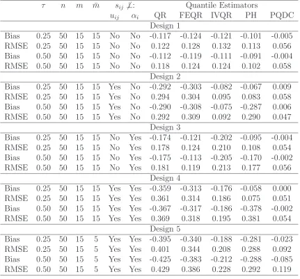
Table A.1 shows results from several quantile regression estimators: (i) a naive quantile
regression approach that uses the censored variable Y (QR), (ii) a fixed effects approach
(FEQR) that while addressing issues of dependence betweenαiandxij ignores censoring, (iii)
an instrumental variable method (IVQR), (iv) the survival approach for a censored quantile
regression model (PH) proposed by Peng and Huang (2008), and (v) the quantile regression
estimator proposed in this paper (PQDC). As in Section 2.2, the estimator is obtained in
two steps. In the first step, we generate the control variable using the least squares residuals
obtained from a parametric regression of the endogenous variable sij on the instrument wij.
The table presents the bias of the estimators and their root mean square error (RMSE) for
the slope β1 = 1 in equation (A.1) at two quantilesτ ={0.25,0.50}, considering n= 50 and
m= 15. The average number of time series observations ¯m=n−1Pn
i=1mi = 5. Tables A.2
and A.3 show additional results for n= 20 and m = 50.
It is important to note that the three procedures (QR, FEQR, IVQR) being compared