Performance of b jet identification in the ATLAS experiment

(1)

This content has been downloaded from IOPscience. Please scroll down to see the full text.

Download details:

IP Address: 148.88.176.169

This content was downloaded on 23/05/2016 at 10:23

Please note that terms and conditions apply.

Performance of b-jet identification in the ATLAS experiment

View the table of contents for this issue, or go to the journal homepage for more 2016 JINST 11 P04008

(http://iopscience.iop.org/1748-0221/11/04/P04008)

(2)

2016 JINST 11 P04008

Published by IOP Publishing for Sissa Medialab

Received:December 3, 2015

Accepted:February 22, 2016

Published:April 4, 2016

Performance of

b

-jet identification in the ATLAS

experiment

The ATLAS collaboration

E-mail: [email protected]

Abstract: The identification of jets containingbhadrons is important for the physics programme of the ATLAS experiment at the Large Hadron Collider. Several algorithms to identify jets containing

bhadrons are described, ranging from those based on the reconstruction of an inclusive secondary vertex or the presence of tracks with large impact parameters to combined tagging algorithms making use of multi-variate discriminants. An independent b-tagging algorithm based on the reconstruction of muons inside jets as well as theb-tagging algorithm used in the online trigger are also presented.

The b-jet tagging efficiency, thec-jet tagging efficiency and the mistag rate for light flavour jets in data have been measured with a number of complementary methods. The calibration results are presented as scale factors defined as the ratio of the efficiency (or mistag rate) in data to that in simulation. In the case ofbjets, where more than one calibration method exists, the results from the various analyses have been combined taking into account the statistical correlation as well as the correlation of the sources of systematic uncertainty.

Keywords: Large detector systems for particle and astroparticle physics; Large detector-systems performance; Pattern recognition, cluster finding, calibration and fitting methods; Performance of High Energy Physics Detectors

(3)

2016 JINST 11 P04008

Contents

1 Introduction 1

2 Data and simulation samples, object selection 2

3 Lifetime-based tagging algorithms 4

3.1 Key ingredients 5

3.2 Impact parameter-based algorithms 6

3.3 Vertex-based algorithms 7

3.4 Combined tagging algorithms 8

3.5 Performance in simulation 13

4 Muon-based tagging algorithm 14

4.1 Muon selection 14

5 b-jet trigger algorithm 16

5.1 Trigger selection 16

6 Dependence of theb-tagging performance on pile-up 18

7 Simulation modelling ofb-tagging input observables 20 7.1 Measurement of the impact parameter resolution of charged particles 20

7.2 Input variable comparisons using fully reconstructedbhadrons 22

7.2.1 Comparison procedure and sample selection 22

7.2.2 Comparison of variables 24

8 b-jet tagging efficiency calibration using muon-based methods 27

8.1 Data and simulation samples 27

8.2 Jet energy correction for semileptonicbdecays 28

8.3 Thep_Trelmethod 28

8.4 The system8 method 30

8.5 Systematic uncertainties 32

8.6 Results 37

9 b-jet tagging efficiency calibration usingt_t¯_{-based methods} ₃₈

9.1 Simulation samples, event selections and background estimates 39

9.1.1 Event selection 39

9.1.2 Selection of the single-lepton sample 40

9.1.3 Background estimation in the single-lepton channel 40

9.1.4 Selection of the dilepton sample 41

(4)

2016 JINST 11 P04008

9.2 Tag counting method 43

9.3 Kinematic selection method 45

9.4 Kinematic fit method 46

9.5 Combinatorial likelihood method 49

9.7 Results 58

9.8 Thep_Trelmethod intt¯events 59

10 Combination ofb-jet efficiency calibration measurements 62

11 b-jet efficiency calibration of the soft muon tagging algorithm 64

11.2 Tag-and-probe based SMT muon efficiency measurement 65

11.3 b-jet tagging efficiency measurement 66

11.4.1 SMT muon efficiency uncertainties 67

11.4.2 b-jet tagging efficiency uncertainties 68

11.5 Results 69

12 c-jet tagging efficiency calibration using events with aWboson produced in association

with acquark 70

12.2 Event selection 72

12.3 Determination of theW+cyield 72

12.4 Measurement of thec-jet tagging efficiency of SMTcjets 75

12.5 Calibration of thec-jet tagging efficiency for inclusivec-jet samples 76

12.7 Results 80

13 c-jet tagging efficiency calibration using theD?method 81

13.2 TheD?analysis 82

13.4 Results 90

14 Mistag rate calibration 91

14.2 The negative tag method 91

14.4 Results 97

15 Mistag rate calibration of the soft muon tagging algorithm 97

(5)

2016 JINST 11 P04008

15.4 Results 100

16 Conclusions 100

The ATLAS collaboration 109

1 Introduction

The identification of jets containingbhadrons is an important tool used in a spectrum of measure-ments comprising the Large Hadron Collider (LHC) physics programme. In precision measuremeasure-ments in the top quark sector as well as in the search for the Higgs boson and new phenomena, the sup-pression of background processes that contain predominantly light-flavour jets using b-tagging is of great use. It may also become critical to achieve an understanding of the flavour structure of any new physics (e.g. supersymmetry) revealed at the LHC.

Several algorithms to identify jets containing bhadrons have been developed, exploiting the long lifetime, high mass and decay multiplicity of bhadrons and the hardb-quark fragmentation function. They range from an algorithm that uses the signed significance of the decay length with respect to the proton-proton collision location, in the following referred to as the primary vertex, of an inclusively reconstructed secondary vertex to more refined algorithms using both secondary vertex properties and the significance of the transverse and longitudinal impact parameters of the charged particle tracks. The most discriminating observables resulting from these algorithms are combined in artificial neural networks. An independentb-tagging algorithm based on reconstructed muons inside jets, exploiting the relatively large fraction ofb-hadron decays with muons in the final state, about 20%, and the b-tagging algorithm used for the online trigger selection have also been developed.

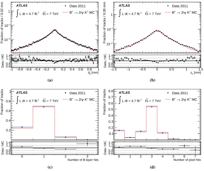
The performance of the tagging algorithms has been characterised in simulated events, includ-ing the dependence on additional proton-proton interactions in the same bunch crossinclud-ing, referred to as pile-up in the following. A first comparison between data and simulation focuses on the basic ingredients forb-tagging, namely the track properties, including the impact parameter distributions. A second comparison focuses more specifically on tracks inbjets, and is made possible by fully reconstructing theb-hadron decayB±→ J/ψK±.

To useb-tagging in physics analyses, the efficiencybwith which a jet containing abhadron is tagged by a b-tagging algorithm needs to be measured. Other necessary pieces of information are the probability of mistakenly tagging a jet containing a c hadron (but not a b hadron) or a light-flavour parton (u-,d-,s-quark or gluong) jet as abjet. In the following, these are referred to as thec-jet tagging efficiency and mistag rate, respectively.

(6)

2016 JINST 11 P04008

to D?+ mesons as well as in a sample of W +c events. The mistag rate has been measured in

an inclusive jet sample. The calibration results are presented as data-to-simulation scale factors, derived from the ratio of the efficiency or mistag rate measured in data to that obtained in simulated events. Where more than one calibration method exists the results from the various analyses have been combined taking into account the statistical and systematic correlation.

This paper is intended to provide a complete description of almost all the b-tagging develop-ments in ATLAS during Run 1 of the LHC in the years 2010 – 2012. The results are illustrated with data taken in the year 2011 at a centre-of-mass energy of 7 TeV. As these developments extended over a period of years, there is some variation between the simulated samples and systematic un-certainties used for the data efficiency measurements depending on the chronology. Also, several of the methods developed to measure the tagging efficiency ofbjets on the small samples available at the start of Run 1 have meanwhile been abandoned in favour of more precise calibration methods developed later; this is reflected in the choice of results used in the combination ofb-jet efficiency measurements made to achieve the ultimate precision. In those methods used previously, quoted values and uncertainties for parameters entering the analysis do reflect the best knowledge at the time. They have not been updated since to benefit from the improved present knowledge on some of the analysis ingredients. Section2starts with a discussion of the data and simulated samples used throughout this paper, along with a description of the corrections applied to the simulated samples to reproduce the experimental conditions present in the data. The variousb-tagging algorithms are described in sections3,4, and5. Section6discusses the effects of pile-up, while section7provides a comparison between data and simulated samples of distributions of selected quantities important for b-tagging. Calibrations of the b-jet tagging efficiency and their combination are discussed in sections8, 9, 10, and11. Calibrations of thec-jet tagging efficiency are covered in sections 12 and13, while the mistag rate calibration is discussed in sections14and15.

2 Data and simulation samples, object selection

The studies presented in this paper are generally based on a data sample corresponding to approxi-mately 4.7 fb−1of 7 TeV proton-proton collision data, after requiring the data to be of good quality; slight differences exist due to variations in data quality requirements. The data have been collected in 2011 using the ATLAS experiment. The ATLAS detector is a large, general-purpose collider detector and is described in detail elsewhere [1]. Its most prominent features, as relevant tob-jet identification and its performance estimation, are:

• An Inner Detector (ID) [2], providing tracking and vertexing capabilities for|η| <2.5.₁ It is immersed in an axial 2 T magnetic field and features three subdetectors employing different techniques. A pixel detector consisting of three layers of silicon pixel sensors is located closest to the beam line. It is followed by a silicon microstrip detector (SCT), consisting of eight (eighteen) layers of silicon microstrip sensors arranged in cylinders (disks) in its barrel (endcap) region, and by a straw tube tracker providing of order 36 measurements for track

(7)

2016 JINST 11 P04008

reconstruction as well as causing high-energy electrons to generate transition radiation.

Espe-cially the pixel and microstrip layers are essential for the purpose of a precise reconstruction of tracks and of displaced vertices.

• A fine-grained lead and liquid argon sampling calorimeter, providing electromagnetic calorimetry up to|η| <3.2.

• A hermetic hadronic calorimeter covering the range |η| < 4.9. Its central part is a steel and scintillating tile sampling calorimeter; its forward parts are again sampling calorimeters, using a liquid argon detection medium and copper and tungsten absorbers.

• A large air-core Muon System (MS), providing stand-alone precision muon momentum reconstruction in the range |η| < 2.7 using a combination of drift tube and resistive plate chamber technologies, and equipped with dedicated detectors for triggering and precise timing. A system of one barrel and two endcap magnet toroids provides a bending power ranging between 1 Tm and 7.5 Tm, lowest in the transition region between the toroids.

A three-level trigger system was used to reduce the event rate from the 20 MHz bunch cross-ing rate to ∼ 200 Hz. The trigger selections used in the different studies are described in the corresponding sections.

The key objects for b-tagging are the calorimeter jets, the tracks reconstructed in the Inner Detector and the signal primary vertex of the hard-scattering collision of interest which is selected from the set of all reconstructed primary vertices. Each vertex is required to have two or more tracks. Tracks are reconstructed from clusters of signals in the silicon pixel and microstrip sensors, and drift circles in the straw tube tracker (collectively referred to as “hits” in the following). They are associated with the calorimeter jets based on their angular separation∆R(track,jet) ≡

p

(∆η)2+₍_∆φ₎2_{. The association}_∆_R_{cut varies as a function of the jet}_p

T, resulting in a narrower

cone for jets at highp_Twhich are more collimated. At 20 GeV, it is 0.45 while for more energetic jets with apT of 150 GeV the∆Rcut is 0.26. Any given track is associated with at most one jet;

if it satisfies the association criterion with respect to more than one jet, the jet with the smallest

∆R is chosen. The track selection criteria depend on the b-tagging algorithm, and are detailed in section3.

(8)

2016 JINST 11 P04008

parameters less than 1.5 mm are considered; it is required to be larger than 0.75. The selection of the

primary vertex is described in section3.1. Some measurements of theb-jet tagging efficiency make use of soft muons (pT > 4 GeV) associated with jets, using a spatial matching of∆R(jet, µ) <0.4.

Multiple Monte Carlo (MC) simulated samples are used throughout this paper. The properties and performance of the tagging algorithms are mostly studied using simulated samples oftt¯events, which unless otherwise stated are generated with MC@NLO v3.41 [7] interfaced to HERWIG v6.520 [8]; for several studies and performance measurements, multijet samples generated using PYTHIA v6.423 [9] are used. To reproduce the pile-up conditions in the data, extra collisions have been superimposed on the simulated events. To simulate the detector response, the generated events are processed through a GEANT4 [10] simulation of the ATLAS detector, and then reconstructed and analysed in the same way as the data. The simulated detector geometry corresponds to a perfectly aligned Inner Detector and the majority of the disabled silicon detector (pixel and strip) modules and front-end chips present in data are masked in the simulation. The ATLAS simulation infrastructure is described in more detail in ref. [11].

To bring the simulation into agreement with data for distributions where discrepancies are known to be present, corrections have been applied to some of the simulated samples. The average number of interactions per bunch crossing, denotedhµi, ranged between 4 and 20 [12]. Its distribution in simulated events has been reweighted to ensure a good agreement in the distribution of the number of reconstructed primary vertices between data and simulation. The fraction of pile-up interactions leading to visible signatures (reconstructible interactions) in the region 2.09 < |η| < 3.84 is computed from refs. [13,14], and is used to scale thehµivalues prior to the reweighting described above, to bring the numbers of reconstructible interactions in agreement between data and simulated events. Applying this scaling has been verified to lead to a good agreement between data and simulated events also in the average number of reconstructed primary vertices as a function ofhµi. When appropriate, thepTspectrum of the simulated jets has also been reweighted to match

the spectrum in data, to account e.g. for the fact that the prescale factors of low threshold jet triggers present in data are not activated in the simulation.

The labelling of the flavour of a jet in simulation is done by spatially matching the jet with generator level partons [15]: if abquark with a transverse momentum of more than 5 GeV is found within∆R(b,jet) < 0.3 of the jet direction, the jet is labelled as abjet. If nobquark is found the procedure is repeated forcquarks andτleptons. A jet for which no such association can be made is labelled as a light-flavour jet.

3 Lifetime-based tagging algorithms

The lifetime-based tagging algorithms take advantage of the relatively long lifetime of hadrons containing a bquark, of the order of 1.5 ps (cτ ≈ 450µm). Abhadron withpT = 50 GeV will

(9)

2016 JINST 11 P04008

longitudinal impact parameter,z0, is the difference between thezcoordinates of the primary vertex

position and of the track at this point of closest approach inr–φ. The tracks fromb-hadron decay products tend to have large impact parameters which can be distinguished from tracks stemming from the primary vertex. Two tagging algorithms exploiting these properties are discussed in this article: JetProb, used mostly for early data, and IP3D for high-performance tagging. The second approach is to reconstruct explicitly the displaced vertices. Two algorithms make use of this technique: the SV algorithm attempts to reconstruct an inclusive secondary vertex; while the JetFitter algorithm aims at reconstructing the completeb-hadron decay chain. Finally, the results of several of these algorithms are combined in the MV1 tagger to improve the light-flavour-jet rejection and to increase the range ofb-jet tagging efficiency for which the algorithms can be applied. These algorithms are discussed in detail in sections3.2–3.4.

3.1 Key ingredients

The determination on an event-by-event basis of the primary vertex [16] is particularly important for b-tagging, since it defines the reference point with respect to which impact parameters and vertex displacements are expressed. The precision of the reconstructed vertex positions improves with increasing associated track multiplicity. For example, in minimum bias events it improves from approximately 300µm (600µm) in thexandy(z) directions for two-track vertices to 20 µm (35µm) for vertices with 70 associated tracks. The vertex resolution depends strongly on the event topology, and significantly better resolutions can be achieved in events with high-pTjets or leptons.

The number of reconstructed primary vertices is substantially larger than one in the presence of pile-up interactions: during the highest instantaneous luminosity of the 2011 data taking period, six primary vertex candidates were reconstructed on average. The adopted strategy is to choose the primary vertex candidate that maximises the sum of the associated tracks’p2_T. The performance of this algorithm depends on the final state and on the pile-up conditions (as will be discussed further in section6); simulation studies indicate that the probability to choose the correct primary vertex intt¯events is higher than 98%, while in lower-multiplicity final states it can be considerably lower. The actual tagging is performed on the sub-set of tracks in the event that are associated with the jet. Once associated with a jet, tracks are subject to specific requirements designed to select well-measured tracks and to reject so-called fake tracks (in which not all hits used for the track reconstruction originate from a single charged particle) and tracks from long-lived particles (K_s,Λ

and other hyperon decays) or material interactions (photon conversions or hadronic interactions). Theb-tagging baseline quality level requires at least seven precision hits (pixel or micro-strip hits) on the track, and at least two of these in the pixel detector, one of which must be in the innermost pixel layer. Only tracks withpT > 1 GeV are considered. The transverse and longitudinal impact

parameters defined with respect to the primary vertex must fulfil |d₀| < 1 mm and |z₀|sinθ < 1.5 mm, whereθis the track polar angle (the factor sinθserves to make the efficiency for tracks to pass these selection criteria less dependent on their polar angles). This selection is used by all the tagging algorithms relying on the impact parameters of tracks. The average number ofb-tagging quality tracks associated to a jet with pT = 50 GeV (200 GeV) is 3.5 (7). In typicaltt¯events, the

average number of selected tracks per light-flavour (bquark) jet is 3.7 (5.5) and their averagepTis

(10)

2016 JINST 11 P04008

decays of long-lived particles; these tracks are subsequently removed forb-tagging purposes. The

main differences in the selection cuts for the SV algorithm are: p_T > 400 MeV,|d₀| <3.5 mm (no cut on z0). The corresponding cuts used by the JetFitter algorithm are: pT > 500 MeV, |d0| < 7

mm,|z0|sinθ <10 mm. Both algorithms make a requirement of at least one hit in the pixel detector

(with no requirement on the innermost pixel layer).

3.2 Impact parameter-based algorithms

For the tagging itself, the impact parameters of tracks are computed with respect to the selected primary vertex. Given that the decay point of the b hadron must lie along its flight path, the transverse impact parameter is signed to further discriminate the tracks fromb-hadron decay from tracks originating from the primary vertex. The sign is defined as positive if the track intersects the jet axis in front of the primary vertex, and as negative if the intersection lies behind the primary vertex. The jet axis is defined by the calorimeter-based jet direction. However if an inclusive secondary vertex is found in the jet (cf. section3.3), the jet direction is replaced by the direction of the line joining the primary and the secondary vertices. The experimental resolution generates a random sign for the tracks originating from the primary vertex, while tracks from theb-/c-hadron decay normally have a positive sign. Decays of e.g.K_s0andΛ0as well as interactions in the detector material also produce tracks with positively signed impact parameters, enhancing the probability to identify light flavour jets asb-quark jets.

JetProb [17] is an implementation of a simple algorithm extensively used at LEP and later at the Tevatron. It uses the track impact parameter significance S_d₀ ≡ d₀/σ_d₀, where σ_d₀ is the uncertainty on the reconstructedd0. TheSd0value of each selected track in a jet,i, is compared to a pre-determined resolution functionR(Sd0)for prompt tracks, in order to measure the probability that the track originates from the primary vertex,P_trk,i, as

P_trk,i=

Z − |Si

d₀|

−∞

R(x)dx. (3.1)

The resolution function is determined from experimental data using the negative side of the signed impact parameter distribution, assuming that the contribution from heavy-flavour particles is negli-gible. The individual track probabilitiesPtrk,ifor theN tracks with positived0 are then combined

as follows:

P_jet=P₀

N−1

X

j=0

(−lnP₀)j

j! , where P0= N Y

i=1

P_trk,i. (3.2)

For light-flavour jets and a perfect suppression of tracks resulting from decays of long-lived hadrons or from material interactions, the distribution ofPjetshould be uniform, while it should peak around

zero forbjets. This robust algorithm with no dependence on simulation was mostly used for data taken before 2011, and is still used for onlineb-tagging (this is discussed in section5).

(11)

2016 JINST 11 P04008

sum of the logarithms of the individual track weights. The LLR formalism allows track categories

to be used by defining different dedicated PDFs for each of them. Currently two exclusive categories are used: the tracks that share a hit in the pixel detector or more than one hit in the silicon strip detector with another track, and those that do not.

3.3 Vertex-based algorithms

To further increase the discrimination between b jets and light-flavour jets, an inclusive three dimensional vertex formed by the decay products of the b hadron, including the products of the possible subsequent charm hadron decay, can be sought. The algorithm starts from all tracks that are significantly displaced from the primary vertex₂and associated with the jet, and forms vertex candidates for track pairs with vertex fit χ2 < 4.5. Vertices compatible with long-lived particles or material interactions are rejected: the invariant mass of the charged-particle track four-momenta is used to reject vertices that are likely to originate from Ks, Λdecays and photon conversions, while the position of the vertex in ther–φprojection is compared to a simplified description of the innermost pixel layers to reject secondary interactions in the detector material. All tracks from the remaining two-track vertices are combined into a single inclusive vertex, using an iterative procedure to remove the track yielding the largest contribution to the χ2of the vertex fit until this contribution passes a predefined threshold.

A simple discriminant between bjets and light-flavour jets is the flight length significance

L₃_D/σ_L₃_D, i.e., the distance between the primary vertex and the inclusive secondary vertex divided by the measurement uncertainty. The significance is signed with respect to the jet direction, in the same way as the transverse impact parameter of tracks is. The flight length significance is the discriminating observable on which the SV0 tagging algorithm relies. As is typical for secondary vertex tagging algorithms, the mistag rate is much smaller than for impact parameter-based algorithms, but the limited secondary vertex finding efficiency, of approximately 70%, can be a drawback.

SV1 is another tagging algorithm based on the same secondary vertex finding infrastructure, but it provides a better performance as it is based on a likelihood ratio formalism, like the one explained previously for the IP3D algorithm. Three of the vertex properties are exploited: the vertex mass(i.e., the invariant mass of all charged-particle tracks used to reconstruct the vertex, assuming that all tracks are pions), the ratio of the sum of the energies of these tracks to the sum of the energies of all tracks in the jet, and the number of two-track vertices. In addition, the∆R

between the jet direction and the direction of the line joining the primary vertex and the secondary vertex is used in the LLR. Some of these properties are illustrated in figure1for bjets,cjets and light-flavour jets in simulatedtt¯events. SV1 relies on a two-dimensional distribution of the first two variables and on two one-dimensional distributions of the latter variables. The secondary vertex finding efficiency depends in particular on the event topology. SV1 requires an a priori knowledge ofSV_b and the corresponding efficiency for light-flavour jets,SV_l , obtained from simulation. This efficiency is shown as a function of the jetp_T in figure1c.

A very different algorithm, JetFitter [15], exploits the topological structure of weak b- and

c-hadron decays inside the jet. A Kalman filter is used to find a common line in three dimensions

2d3D/σd3D >2, whered3Dis the three dimensional distance between the primary vertex and the point of closest

(12)

2016 JINST 11 P04008

SV mass [GeV]

0 1 2 3 4 5 6

Fraction of jets / 0.06 GeV

5 − 10 4 − 10 3 − 10 2 − 10 1 − 10 t =7 TeV, t s

|<2.5 jet

η >20 GeV, | jet T p b jets c jets light-flavour jets ATLAS Simulation (a)

SV energy fraction

0 0.2 0.4 0.6 0.8 1

Fraction of jets / 0.008

5 − 10 4 − 10 3 − 10 2 − 10 1 − 10 t =7 TeV, t s

|<2.5 jet

η >20 GeV, | jet T p b jets c jets light-flavour jets ATLAS Simulation (b) [GeV] T jet p 50 100 150 200 250 300 350 400 450 500

SV finding efficiency

0 0.1 0.2 0.3 0.4 0.5 0.6 0.7 0.8 t =7 TeV, t s

|<2.5 jet

η >20 GeV, | jet T p b jets c jets light-flavour jets ATLAS Simulation (c)

Figure 1. The vertex mass (a), energy fraction (b) and vertex finding efficiency (c) of the inclusive secondary vertices found by the SV1 algorithm, for three different flavours of jets.

on which the primary vertex and the bottom and charm vertices lie, as well as their positions on this line approximating theb-hadron flight path. With this approach, theb- andc-hadron vertices are not merged, even when only a single track is attached to each of them. In the JetFitter algorithm, the decay topology is described by the following discrete variables: the number of vertices with at least two tracks, the total number of tracks at these vertices, and the number of additional single track vertices on the b-hadron flight axis. The vertex information is condensed in the following observables, shown in figure2: the vertex mass (the invariant mass of all charged particle tracks attached to the decay chain), the energy fraction (the energy of these charged particles divided by the sum of the energies of all charged particles associated to the jet), and the flight length significanceL/σL(the average displaced vertex decay length divided by its uncertainty; the individual reconstructed vertices contribute to the average decay length weighted by the inverse square of their decay length uncertainties). The six JetFitter variables defined above are used as input nodes in an artificial neural network. As the input variable distributions depend on thepTand|η|of

the jets, these kinematic variables are included as two additional input nodes. To ensure that the jet

pTand|η|spectra of theb,cand light-flavour jets in the training sample are not used by the neural

network to separate the different jet flavours, a two-dimensional reweighting yielding flat kinematic distributions for all three jet flavours is performed prior to the neural network training. A coarse two-dimensional binning with seven bins in pT and three bins in |η| is used for the reweighting.

The JetFitter neural network has three output nodes, corresponding to theb-,c- and light-flavour-jet hypotheses, referred to asP_b,P_c andP_l. The network topology includes two hidden layers, with 12 and 7 nodes, respectively. A discriminating variable to selectbjets and reject light-flavour jets is then defined from the values of the corresponding output nodes: wJetFitter=ln(Pb/Pl).

3.4 Combined tagging algorithms

(13)

2016 JINST 11 P04008

Mass [GeV]

0 1 2 3 4 5 6 7 8

0 0.01 0.02 0.03 0.04 0.05 2 tracks

3 or more tracks

ATLAS Simulation, b jets

[image:13.595.91.503.95.447.2]

t =7 TeV, t s

|<2.5 jet

η >20 GeV, | jet T p

(a)

Mass [GeV] 0 1 2 3 4 5 6 7 8

0 0.02 0.04 0.06 0.08 0.1 2 tracks

3 or more tracks

ATLAS Simulation, c jets

t =7 TeV, t s

|<2.5 jet

(b)

Mass [GeV] 0 1 2 3 4 5 6 7 8

0 0.02 0.04 0.06 0.08 0.1 0.12 2 tracks

3 or more tracks

ATLAS Simulation, light-flavour jets

t =7 TeV, t s

|<2.5 jet

(c)

Energy fraction 0 0.1 0.2 0.3 0.4 0.5 0.6 0.7 0.8 0.9 1

0.02 0.04 0.06 0.08 0.1

0.12 1 single track 2 single tracks 2 tracks 3 or more tracks

t =7 TeV, t s

|<2.5 jet

(d)

Energy fraction 0 0.1 0.2 0.3 0.4 0.5 0.6 0.7 0.8 0.9 1

0.02 0.04 0.06 0.08 0.1 0.12

1 single track 2 single tracks 2 tracks 3 or more tracks

t =7 TeV, t s

|<2.5 jet

(e)

Energy fraction 0 0.1 0.2 0.3 0.4 0.5 0.6 0.7 0.8 0.9 1

0.05 0.1 0.15 0.2 0.25 0.3 t =7 TeV, t s

|<2.5 jet

1 single track 2 single tracks 2 tracks 3 or more tracks

(f)

Weighted flight length significance 0 5 10 15 20 25

0.02 0.04 0.06 0.08 0.1 0.12 0.14 0.16 0.18 No vertex

1 or more vertices

t =7 TeV, t s

|<2.5 jet

(g)

0.05 0.1 0.15 0.2 0.25 No vertex

1 or more vertices

t =7 TeV, t s

|<2.5 jet

(h)

0.02 0.04 0.06 0.08 0.1 0.12 0.14 0.16 0.18 0.2 0.22 No vertex

1 or more vertices

t =7 TeV, t s

|<2.5 jet

(i)

Figure 2. The vertex mass (top), energy fraction (middle) and flight length significance (bottom) forbjets (left), cjets (middle) and light-flavour jets (right), split according to the decay chain topology found by JetFitter. In the case that no vertex with at least two outgoing tracks has been reconstructed, these quantities are computed from reconstructed single track vertices as explained in the text. The distributions are obtained from a simulated sample oftt¯events generated with POWHEG [18,19] interfaced to PYTHIA.

respective weights: this is the so-called IP3D+SV1 algorithm. Another combination technique is the use of an artificial neural network, which can take advantage of complex correlations between the input values. Two tagging algorithms are defined in this way, IP3D+JetFitter and MV1.

The IP3D+JetFitter algorithm is defined in the same way as the JetFitter algorithm itself, with the only difference being that the output weight of the IP3D algorithm is used as an additional input node, and that the number of nodes in the two intermediate hidden layers is increased to 9 and 14, respectively. The discriminating variable to selectbjets and reject light-flavour jets is defined as

wIP3D+JetFitter = ln(Pb/Pl). A specific tuning of the IP3D+JetFitter algorithm to provide a better discrimination betweenbandcjets useswIP3D+JetFitter(c)=ln(Pb/Pc)as a discriminant.

(14)

2016 JINST 11 P04008

IP3D weight

40

− −30−20−10 0 10 20 30 40 50 60

Fraction of jets

6 − 10 5 − 10 4 − 10 3 − 10 2 − 10 1 − 10

1 _s_{=7 TeV, t}_t

>20 GeV, jet T p |<2.5 jet η | b jets c jets light-flavour jets ATLAS Simulation (a) 4

− −2 0 2 4 6 8 10 12

5 − 10 4 − 10 3 − 10 2 − 10 1 − 10 1 SV1 weight t

=7 TeV, t s

|<2.5 jet

η >20 GeV, | jet T p b jets c jets light-flavour jets ATLAS Simulation (b) 8

− −6 −4 −2 0 2 4 6 8

5 − 10 4 − 10 3 − 10 2 − 10 1 − 10 1 IP3D+JetFitter weight t

=7 TeV, t s

|<2.5 jet

η >20 GeV, | jet T p b jets c jets light-flavour jets ATLAS Simulation (c)

Figure 3. Distribution of the IP3D (a), SV1 (b) and IP3D+JetFitter (c) weights, forb,cand light-flavour jets. These three weights are used as inputs for the MV1 algorithm. The spikes atwIP3D ≈ −20 and≈ −30

correspond to pathological cases where the IP3D weight could not be computed, due to the absence of good-quality tracks. The spike at wSV1 ≈ −1 corresponds to jets in which no secondary vertex could be

reconstructed by the SV1 algorithm, and where discrete probabilities for aband light-flavour jet not to have a vertex are assigned. The irregular behaviour inwIP3D+JetFitterarises because both thewIP3Dand thewJetFitter

distribution (not shown) exhibit several spikes.

The distributions of the correlations between the three input weights are also shown in figure4, for

bjets,cjets and light-flavour jets. These distributions illustrate the potential gain in combining the three weights: it can be seen that the IP3D weight has only limited correlations with the secondary vertex-based weights, while naturally SV1 and IP3D+JetFitter weights are more correlated but the correlation is different in theb-jet,c-jet and light-flavour-jet samples. The MV1 neural network is a perceptron with two hidden layers consisting of three and two nodes, respectively, and an output layer with a single node which holds the final discriminant variable. The implementation used is the MLP code from the TMVA package [20]. The training relies on a back-propagation algorithm and is based on two simulated samples ofbjets (signal hypothesis) and light-flavour jets (background hypothesis). Most of the jets are obtained from simulatedtt¯events and their average transverse momentum is around 60 GeV. To provide jets with higherp_Tfor the training, simulated dijet events with jets in the 200 GeV < pT < 500 GeV range are also included. As in the case of the JetFitter

neural network, since the tagging performance depends strongly on the pTand, to a lesser extent,

on theηof the jet, biases may arise from the different kinematic spectra of the two training samples (of light-flavour andbjets). To reduce this effect, weighted training events are used. Each jet is assigned to a category defined by a coarse two-dimensional grid in(pT, η)with four bins inηand

(15)

2016 JINST 11 P04008

7 − 10 6 − 10 5 − 10 4 − 10 3 − 10 2 − 10 1 − 10 SV1 weight 4

− −2 0 2 4 6 8 10 12

IP3D weight 40 − 30 − 20 − 10 − 0 10 20 30 40 50 60

[image:15.595.94.510.149.606.2]

t = 7 TeV, t s

| < 2.5

jet η

> 20 GeV, |

jet T p (a) IP3D+JetFitter weight 8

− −6 −4 −2 0 2 4 6 8

IP3D weight 40 − 30 − 20 − 10 − 0 10 20 30 40 50 60 7 − 10 6 − 10 5 − 10 4 − 10 3 − 10 2 − 10 1 − 10

t = 7 TeV, t s

| < 2.5

jet η

> 20 GeV, |

jet T p (b) 7 − 10 6 − 10 5 − 10 4 − 10 3 − 10 2 − 10 1 − 10 SV1 weight 4

− −2 0 2 4 6 8 10 12

IP3D+JetFitter weight 8 − 6 − 4 − 2 − 0 2 4 6 8

t = 7 TeV, t

s _ηjet| < 2.5 > 20 GeV, |

jet T p (c) 7 − 10 6 − 10 5 − 10 4 − 10 3 − 10 2 − 10 1 − 10 SV1 weight 4

− −2 0 2 4 6 8 10 12

IP3D weight 40 − 30 − 20 − 10 − 0 10 20 30 40 50 60

t = 7 TeV, t s

| < 2.5

jet η

> 20 GeV, |

jet T p (d) 7 − 10 6 − 10 5 − 10 4 − 10 3 − 10 2 − 10 1 − 10 IP3D+JetFitter weight 8

− −6 −4 −2 0 2 4 6 8

IP3D weight 40 − 30 − 20 − 10 − 0 10 20 30 40 50 60

t = 7 TeV, t s

| < 2.5

jet η

> 20 GeV, |

jet T p (e) 7 − 10 6 − 10 5 − 10 4 − 10 3 − 10 2 − 10 1 − 10 SV1 weight 4

− −2 0 2 4 6 8 10 12

t = 7 TeV, t

s _ηjet| < 2.5 > 20 GeV, |

jet T p (f) 7 − 10 6 − 10 5 − 10 4 − 10 3 − 10 2 − 10 1 − 10 SV1 weight 4

− −2 0 2 4 6 8 10 12

IP3D weight 40 − 30 − 20 − 10 − 0 10 20 30 40 50 60

t = 7 TeV, t s

| < 2.5

jet η

> 20 GeV, |

jet T p (g) 7 − 10 6 − 10 5 − 10 4 − 10 3 − 10 2 − 10 1 − 10 IP3D+JetFitter weight 8

− −6 −4 −2 0 2 4 6 8

IP3D weight 40 − 30 − 20 − 10 − 0 10 20 30 40 50 60

t = 7 TeV, t s

| < 2.5

jet η

> 20 GeV, |

jet T p (h) 7 − 10 6 − 10 5 − 10 4 − 10 3 − 10 2 − 10 1 − 10 SV1 weight 4

− −2 0 2 4 6 8 10 12

t = 7 TeV, t

s _ηjet| < 2.5 > 20 GeV, |

jet T

p

(i)

Figure 4. Distributions of the correlations between the IP3D, SV1 and IP3D+JetFitter weights, forbjets (top),cjets (middle) and light-flavour jets (bottom). The spikes atwIP3D ≈ −20 and≈ −30 correspond to

pathological cases where the IP3D weight could not be computed, due to the absence of good-quality tracks. The spike atwSV1≈ −1 corresponds to jets in which no secondary vertex could be reconstructed by the SV1

(16)

2016 JINST 11 P04008

0 0.2 0.4 0.6 0.8 1

5 − 10 4 − 10 3 − 10 2 − 10 1 − 10 MV1 weight

b jets

c jets

light-flavour jets

ATLAS Simulation

[image:16.595.312.506.118.315.2] [image:16.595.307.507.434.628.2]

t =7 TeV, t s

|<2.5

jet η

>20 GeV, |

jet T

p

Figure 5.Distribution of the tagging weight obtained with the MV1 algorithm, for three different flavours of jets.

b-jet tagging efficiency

0.3 0.4 0.5 0.6 0.7 0.8 0.9 1

Light-flavour-jet rejection 1 10 2 10 3 10 4 10 MV1 IP3D+JetFitter IP3D+SV1 JetFitter IP3D SV1 JetProb t =7 TeV, t s

|<2.5

jet

η >20 GeV, |

jet T

p

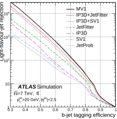
Figure 6.Light-flavour-jet rejection versusb-jet tag-ging efficiency, for various tagtag-ging algorithms.

0 100 200 300 400 500 200 400 600 800 1000 1200 1400 [GeV] T Jet p Light-flavour-jet rejection =60% b ε MV1, =70% b ε MV1, t =7 TeV, t s

|<2.5

jet η

>20 GeV, |

jet T

p

Figure 7. Light-flavour-jet rejection versus jet pT,

for the MV1 algorithm. In each bin the cut on the

b-tagging weight is adjusted to maintain an average 60% (70%)b-jet tagging efficiency.

0 0.5 1 1.5 2 2.5

200 400 600 800 1000 1200 | jet η | Light-flavour-jet rejection =60% b ε MV1, =70% b ε MV1, t =7 TeV, t s

|<2.5

jet η

>20 GeV, |

jet

T

p

Figure 8. Light-flavour-jet rejection versus jet |η|, for the MV1 algorithm. In each bin the cut on the

(17)

2016 JINST 11 P04008

0.3 0.4 0.5 0.6 0.7 0.8 0.9 1 1

10

2

10

c-jet rejection

IP3D+JetFitter(c) IP3D+JetFitter MV1

[image:17.595.92.289.88.282.2] [image:17.595.311.507.89.281.2]

t =7 TeV, t s

|<2.5

jet η

>20 GeV, |

jet T

p

Figure 9. c-jet rejection versus b-jet tagging effi-ciency, for three tagging algorithms.

0.3 0.4 0.5 0.6 0.7 0.8 0.9 1 1

10

2

10

3

10

tau-jet rejection

IP3D+JetFitter MV1

t =7 TeV, t s

|<2.5

jet η

>20 GeV, |

jet

T

p

Figure 10. τ-jet rejection versus b-jet tagging effi-ciency, for two tagging algorithms.

3.5 Performance in simulation

The performance of the tagging algorithms is estimated in large samples of simulated tt¯events. Figure6shows the light-flavour-jet rejection as a function ofb-jet tagging efficiency. As expected, a clear hierarchy between the standalone and combined algorithms is observed. In particular, the use of a combined tagging algorithm can improve the rejection by a factor 4 to 10 compared to JetProb in the 60–80% efficiency range.

For physics analyses it is important to understand the light-flavour-jet rejection as a function of kinematic variables. Figures7and8show the dependence on jet pT andη, respectively. The

rejection is best at intermediate p_Tjet values and in the central region. At low pT and/or high |η|,

the performance is degraded mostly because of the increase of multiple scattering and secondary interactions. For pT greater than about 200 GeV, some dilution arises because the fraction of

fragmentation tracks increases, and morebhadrons fly beyond the first pixel layer. In addition, a further performance degradation results from pattern recognition issues in the core of very dense jets. As mentioned in the previous section, algorithms such as IP3D+JetFitter can be tuned to achieve a better charm rejection. For high-performanceb-tagging algorithms, the ability to rejectcjets also becomes important. Charm hadrons have sufficiently long lifetimes to also lead to reconstructible secondary vertices. Since JetFitter relies not only on the long lifetimes ofbandchadrons but also on the full decay topology, it can help to discriminatebjets andcjets, for instance by separatingb

jets with cascade charm decays (i.e. at least 2 vertices) from single-vertexcjets. The neural network used for the IP3D+JetFitter combination has three output neurons: one for each of the light-quark,b

(18)

2016 JINST 11 P04008

Since hadronic decays ofτ leptons can be reconstructed as jets which can mimicbjets, it is

useful to know the discrimination power betweenτ jets andbjets. This is shown in figure10for two tagging algorithms.

4 Muon-based tagging algorithm

Decays ofbhadrons to muons, either direct,b→µ−, or through the cascade,b→c→µ+(or, with significantly smaller rate,b→c¯→µ−), can be exploited to identifybjets.₃ The intrinsic efficiency of muon-based tagging algorithms is typically lower than that of lifetime-based tagging algorithms due to the limited branching fraction of bhadrons to muons (≈ 20%, including both direct and cascade decays). TheSoft Muon Tagger(SMT), which is described in this section, is a muon-based tagging algorithm that does not use any lifetime information. This makes it complementary to the lifetime-based techniques and subject to significantly different sources of systematic uncertainties.

4.1 Muon selection

The muons considered for tagging in the SMT algorithm are required to be reconstructed both in the ID and the MS, so-called combined muons [1]. Such muons must satisfy track quality requirements on the number of hits in the different ID sub-detectors, aimed at reducing the number of light-flavour hadron decays in flight. Candidate muons also have to be loosely compatible with the reconstructed primary vertex, in order to reject charged particles from additional proton collisions, especially at high LHC instantaneous luminosities, or from nuclear interactions of the hard collision products with the detector material. A candidate muon is associated with a jet if∆R(jet, µ) < 0.5. If more than one jet fulfils this requirement, the muon is associated with the nearest jet only. The candidate muon must further fulfil a set of selection criteria, referred to as SMT selection criteria in the following: |d0| <3 mm,|z0·sinθ| <3 mm and pT> 4 GeV.

Light charged mesons (π±,K±) decay predominantly into muons and thus contribute signifi-cantly to a sample of jets with associated muons. Given the long lifetimes of light charged mesons, a small fraction of those mesons decay between the end of the ID volume and the entrance of the muon system. While in those cases the ID measures the track parameters for the meson, the MS is sensitive to the track of the muon produced in the decay, giving rise to an enlarged χ2for the combination of both measurements. In order to discriminate betweenband light-flavour jets the SMT therefore uses the χ2 of the statistical combination of the track parameters of muons reconstructed in the ID and MS, χ2_match, normalised to the number of degrees of freedom. The momentum imbalance and kink from the decay between the light charged meson and daughter muon will result in χ2_match values larger on average than for decays of heavy-flavoured hadrons. The χ2_matchis defined as

χ2 match=

1

5(P~ID−P~MS)

T_(W

ID+WMS)−1(P~ID−P~MS), (4.1)

where P~ID andP~MS are the 5-dimensional vectors of the trajectory helix parameters measured in

the ID and MS, respectively, andWIDandWMSare their associated 5×5 covariance matrices.

The χ2_match distribution for the different flavour sources in simulated tt¯events is shown in figure 11. Compared to bor c jets, light-flavour jets indeed show a significantly broader χ2_match

(19)

2016 JINST 11 P04008

dof

/N

match 2

χ

0 1 2 3 4 5 6 7 8 9 10

0 0.01 0.02 0.03 0.04 0.05 0.06

b jets

c jets

light-flavour jets

t =7 TeV, t s

|<2.5

jet η >20 GeV, |

jet T

p

Figure 11. Distribution of the χ2_match variable forb (solid green), c(long-dashed blue) and light-flavour (dashed red) jets.

distribution. A jet is considered tagged by the SMT if it has an associated candidate muon passing the SMT selection criteria, which also include the requirement χ2_match <3.2.

Various aspects of the performance of the SMT algorithm have been studied in simulated events of different physics processes.

An inclusive sample of di-muon events from J/ψmeson andZboson decays has been used to provide a clean source of genuine muons spanning a wide transverse momentum range. This allows studies of the efficiency of the SMT selection criteria for isolated muons, including the χ2_matchcut. This efficiency, which is found to be on average around 95%, has been studied as a function of the muon transverse momentum and pseudorapidity. It is found not to depend significantly on the transverse momentum, and exhibit only a mild dependence on the pseudorapidity.

The efficiency of the SMT algorithm to identifybandcjets has been evaluated using a sample of simulatedtt¯events. The averageb- andc-jet tagging efficiencies in this sample are found to be 11.1% and 4.4%, respectively. The efficiencies as a function of jetpT are given in figure12. As

expected, the tagging efficiencies are significantly lower than what is typically found for lifetime-based tagging algorithms, due to the limited branching ratio of muonicb- andc-hadron decays. A dependence on the jetpTis observed, whereby a lower efficiency is found for lowerpT: softer jets

originate from decays of bhadrons with lower transverse momentum, which in turn produce less energetic tagging muons. The latter are more likely to fail the SMT pre-selection requirement on the muon pT (pT> 4 GeV). The efficiency becomes almost flat when jets attain apT range where

they produce high transverse momentum muons.

(20)

2016 JINST 11 P04008

through the calorimeters and nuclear interactions of particles within a jet with the material in the

calorimeters, mimicking muons in the MS. The values of the mistag rate, determined as a function of jetpT and|η|, are summarised in figure13. They are found to be very low, demonstrating the

power of the SMT tagging algorithm.

[GeV]

T

Jet p 20 40 60 80 100 120 140 160

b/c-jet tagging efficiency

0 0.02 0.04 0.06 0.08 0.1 0.12 0.14 0.16

b jets c jets

t = 7 TeV, t s

| < 2.5

jet

η

> 20 GeV, |

jet T

p

[GeV]

T

Jet p

2

10

Mistag rate

0 0.001 0.002 0.003 0.004 0.005

| < 1.2

jet

η

|

| < 2.5

jet

η

1.2 < |

= 7 TeV, inclusive jets s

> 20 GeV

jet T

p

Figure 12. b- and c-jet tagging efficiencies of the SMT algorithm, and associated statistical uncertain-ties.

Figure 13.Mistag rate of the SMT algorithm, and as-sociated statistical uncertainties, for light-flavour jets.

5 b-jet trigger algorithm

The possibility to identifybjets at trigger level is crucial for physics processes with purely hadronic final states containingbjets because the absence of leptons and the huge inclusive jet background make other trigger selections very challenging.

5.1 Trigger selection

Theb-jet trigger selection starts from the calorimetric jet candidates, reconstructed by the hardware-based first level trigger (LVL1); the corresponding charged-particle tracks, reconstructed by the two subsequent software-based trigger levels, the second level trigger (LVL2) and the Event Filter (EF), are then analysed with lifetime-based algorithms. For a detailed description of the ATLAS trigger scheme, including the detailed descriptions of tracking, vertexing and beamspot determination in the trigger, see ref. [21].

During the 2011 data taking, theb-tagging trigger selection was based on the impact parameter significance of the reconstructed tracks. The tagging algorithm adopted for the primary physics trigger was an online version of the JetProb algorithm described in section 3.2, applied to jet candidates identified by the LVL1 trigger. To maximise the acceptance for different physics channels, various b-jet trigger selections were deployed during 2011 data taking, differing in LVL1 jet requirements as well as inb-tagging requirements. The trigger selections required either a single or multipleb-tagged jets, and thebjets were selected at three working points. These working points, referred to astight, mediumandloose, correspond respectively to approximately 40%, 55% and 70% identification efficiency for selecting jets corresponding to true offlinebjets, measured on a

(21)

2016 JINST 11 P04008

EF, which offers a better correlation between online and offline jet pT, to reduce further the rate

without compromising the jet trigger efficiency plateau of the LVL1 selection. The rate reduction provided solely by the request of onetight(twomedium)b-tagged jet(s) is a factor of 6 (13) at LVL2 and 2 (4) at EF.

The data collected in 2011 are compared to a PYTHIA generated dijet sample, and distributions of basic ingredients for theb-jet triggers are shown in figure14. The overall agreement is good but to take into account deviations in the simulation, especially in the impact parameter tails, data-driven techniques will be employed to derive data-to-simulation scale factors, as described in sections8,13 and14.

Signed transverse impact parameter 10

− −5 0 5 10

Entries / 0.1

2

−

10

1

−

10 1 10

2

10

3

10

4

10

5

10

ATLAS

= 7 TeV s

Data 2011 b jets c jets light jets

(a)

Track multiplicity 0 2 4 6 8 10 12 14 16 18 20

Entries

1 10

2

10

3

10

4

10

5

10

6

10

ATLAS

= 7 TeV s

(b)

[GeV]

T

Track p 0 5 10 15 20 25 30

Entries / GeV

2

10

3

10

4

10

5

10

ATLAS

= 7 TeV s

(c)

Figure 14. Signed transverse impact parameter significance (a), multiplicity (b) and transverse momentum (c) of EF tracks that are reconstructed starting from a low-pTjet identified by the LVL1 and are requested

to satisfy online b-tagging criteria. Theb, cand light-flavour distributions are derived from a simulated dijet sample.

The different tagging methods are characterised, at each trigger level, as a curve showing the light-flavour-jet rejection (Rl) versus the efficiency to selectbjets (b). The characterisation of trigger selections also involves studying the bias that each trigger level imposes on the next one and on the final recorded sample. In particular, for theb-jet triggers, this can be derived as an additional rejection versus efficiency curve for offline tagging algorithms, measured on a sample selected by a singleb-jet trigger.

The combined rejection versus efficiency curves for the LVL2, EF and offline selections based on JetProb and measured in a sample of HERWIG generatedtt¯events are shown in figure15; the EF (offline) performance is shown starting from thetightandmediumL2 (EF) working points.

(22)

2016 JINST 11 P04008

about 40%. However the use of theb-jet trigger is not limited to this unbiased offline sample since

data-to-simulation efficiency scale factors are derived for trigger selection and for combined trigger and offline selections.

0.3 0.4 0.5 0.6 0.7 0.8 0.9 1

Light-flavour jet rejection

1 10 100

L2 EF after L2 Offline after HLT Offline

ATLAS Simulation t =7TeV, t s

(a)

0.3 0.4 0.5 0.6 0.7 0.8 0.9 1

Light-flavour jet rejection

1 10 100

L2 EF after L2 Offline after HLT Offline

ATLAS Simulation t =7TeV, t s

(b)

Figure 15. The combined rejection versus efficiency curves for the LVL2, EF and offline JetProb tagging algorithms for the tight (a) and medium (b) trigger working points. The offline rejection versus efficiency curve, measured on an unbiased sample, is superimposed, providing an estimate of the correlation between online and offline selections. The offline jets are required to have |η| < 2.5 and transverse momentum pT>50 GeV (corresponding to the full acceptance of the jet trigger).

6 Dependence of the b-tagging performance on pile-up

With the increasing instantaneous luminosity of the LHC during 2011 data taking, the rate of pile-up interactions increased substantially with an average of 12 interactions per bunch crossing in the later data taking periods, reaching maximum values of more than 20 interactions. These additional interactions can potentially affect theb-tagging performance through several effects:

(23)

2016 JINST 11 P04008

fraction of tracks in the tails of the longitudinal impact parameter distribution is increased,

which also degrades the b-tagging performance. Studies in ref. [22] have shown that the fraction oftt¯events with a misidentified primary vertex is below 2% for the number of addi-tional interactions as present during data taking in 2011. The resolution of thez coordinate of the signal vertex degrades by about 10% for an average of 12 additional interactions as in the later data taking periods in 2011. As explained in section2, a requirement on the jet vertex fraction has been applied to jets selecting only jets for theb-tagging analyses that are compatible with the selected primary event vertex. As a result, jets from the hard scatter interaction that are lost when the wrong primary vertex is selected as signal vertex do not enter into the determination of the performance ofb-tagging algorithms. The consequences of this depend strongly on the specific analysis considered and are not discussed in detail in this paper.

• The increased density of charged particle tracks in the inner tracking detectors makes track reconstruction more challenging. An increased rate of falsely associated hits or hits shared with other tracks, as well as an increased rate of fake tracks are the most important conse-quences. Furthermore, misassociated hits can lead to tails in the impact parameter resolutions for these tracks. These aspects have been studied in refs. [22, 23]. It has been found that for the pile-up conditions in the 2011 data, there is no significant degradation of the track reconstruction efficiency and the track impact parameter resolution in the transverse plane. However, there is some increase of the rate of fake tracks and a slight worsening of the track impact parameter resolution along thezdirection.

• Pile-up interactions can create additional jets reconstructed in the detector. If the correspond-ing interaction vertex is close to the primary vertex of the hard scatter process of interest, charged particle tracks stemming from the pile-up interaction might be falsely associated to the hard scatter primary vertex and mimic lifetime signatures leading to an increased misiden-tification rate of non-bjets. If the pile-up jet overlaps with a signal jet, tracks from the pile-up interaction might be misassociated with the signal jet, diluting theb-tagging performance. Studies in ref. [22] have shown that this is the main source of an increased multiplicity of tracks in signal jets in the presence of pile-up. If the pile-up vertex is sufficiently displaced from the hard scatter vertex, the corresponding tracks will be rejected by the selection criteria, typically not causing false identification of the pile-up jets.

The dependence of theb-tagging performance on the number of reconstructed primary vertices has been studied using simulatedtt¯events. An important input to theb-tagging algorithms is the information from the reconstruction of inclusive secondary decay vertices in jets. The secondary vertex reconstruction can be affected by additional tracks from pile-up vertices. Figure16shows the rate with which secondary vertices are reconstructed by the SV1 algorithm in jets of different flavour, normalised to the average secondary vertex reconstruction rate. It can be seen that forcand

(24)

light-2016 JINST 11 P04008

flavour jets for ab-jet tagging efficiency of 70% versus the number of reconstructed primary vertices

for the MV1 algorithm forttevents. It can be seen that the light-flavour-jet rejection degrades with increasing number of pile-up interactions, resulting in a light-flavour-jet rejection rate that is reduced by a factor of almost two for the highest level of pile-up as present in the year 2011.

Number of primary vertices 0 5 10 15 20

Normalised SV rate

0.8 1 1.2 1.4 1.6

b jets c jets light-flavour jets

Simulation ATLAS

t = 7 TeV, t s

| < 2.5 jet

η > 15 GeV, | jet T p

(a)

Number of primary vertices 0 2 4 6 8 10 12 14 16 18 20

Light-flavour-jet rejection

50 100 150 200 250

Simulation ATLAS

t = 7 TeV, t s

| < 2.5 jet

η > 15 GeV, | jet T p

= 70% b

ε MV1,

(b)

Figure 16. The dependence of the secondary vertex reconstruction rate of the SV1 algorithm (a) and the light-flavour jet rejection of the MV1 algorithm (b) on the number of reconstructed primary vertices, estimated from simulatedttevents. The secondary vertex reconstruction rate has been normalised to the rate in the inclusive sample.

7 Simulation modelling of b-tagging input observables

An acurate modelling of theb-tagging performance in the simulation is based on a correct description of the underlying quantities, such as the reconstruction efficiency and fake rate of tracks and vertices, and the properties of the reconstructed objects. In this section, a comparison between data and simulation is presented for a number ofb-tagging input observables.

7.1 Measurement of the impact parameter resolution of charged particles

Two key ingredients for discriminating between tracks originating from displaced vertices and those originating from the primary vertex are: the transverse impact parameter (IP) of a track,d₀, and

z0sinθ, the longitudinal impact parameter projected onto the direction perpendicular to the track.

Both of these quantities can be measured with respect to the primary vertex in an unbiased way (d_PVandz_PVsinθ): if the track under consideration was used for the primary vertex determination, it is first removed from the primary vertex which is subsequently refitted, and the impact parameters are computed with respect to this new vertex.

(25)

2016 JINST 11 P04008

position: σ2_IP=σ2

IPtrack+σ

2

PV, whereσPV2 is the projection of the primary vertex uncertainty along

the axis of closest approach of the track to the primary vertex on the transverse or longitudinal plane. In this section, a measurement of the impact parameter resolution in data is presented. Since the measurement does not require a high-luminosity sample, and to limit pile-up effects, only the first runs of the collected data in 2011 are used.

The data were required to satisfy standard ID data quality requirements. The simulation samples considered are PYTHIA generated dijet samples. Events passing a logical OR of inclusive jet triggers, with at least 10 tracks used in the primary vertex reconstruction are retained for this study.

Tracks fulfilling the following basic track quality selection are used:

• The track must be included in the primary vertex reconstruction.

• pT> 500 MeV.

• |η| <2.5.

• >2 hits in the pixel detector.

• >7 hits in the combined pixel and SCT detectors.

In order to extract the correct impact parameter resolution from data it is important to understand how to subtract the contribution from the resolution on the position of the reconstructed primary vertex. Since the primary vertex fit uses the beam spot constraint, the beam spot size is already included in the estimated uncertainty on the primary vertex position. The tracks are divided into different categories ofη,p_T√sinθ, and the number of innermost pixel layer hits to ensure an almost constant resolution within a single category. Both thed0andz0sinθresolution have been measured

for each track category. The pseudorapidityηis chosen as it reflects the kinematics of the particle production mechanism whileθ is more suitable for parametrising detector-related effects. Finally,

pT

√

sinθhas been chosen instead ofpTitself because it is directly linked to the multiple scattering

contribution to the impact parameter resolution in the case that the material traversed by charged particles follows a cylindrical geometry. The resolution is modelled as

σd0 =

s

a2+ b2

p2_sinθ3. (7.1)

The method used to subtract the primary vertex reconstruction contribution to the IP resolution, σPV, relies on an iterative deconvolution procedure. For each iteration it is possible to obtain the

deconvolved distribution by multiplying the measured impact parameter of each track by a correction factor. For example, for the transverse impact parameter with respect to the primary vertex:

d_PV →d_PV s

(Kσd0)2

(Kσd0)2+σ

2 PV

, (7.2)

whereKis a correction factor that depends on the iteration index. For the first iterationK is equal to one. For each iteration,σdPV can be evaluated by fitting eachdPV distribution and for thei-th iteration it should be:

(σdPV)i = Kiσd0 v t

(Ki+1σd0)2+σ

2 PV (Kiσd0)2+σ

2 PV

(26)

2016 JINST 11 P04008

which can then be used to calculateKi+1. To evaluate the width of the core of thedPVdistributions,

and hence estimate the impact parameter resolution, a Gaussian fit is first applied to the whole distribution, and a temporary mean and width are obtained. A new fit range, of width four times the temporary fit width, is then centred around the temporary mean; finally the distribution is refitted within this new range. The iterative procedure ends when the fitted σdPV is stable within approximately 0.01%. About five iterations are needed to make the K factor converge to stable values that range between 0.8 and 1.2. This iterative procedure was verified on Monte Carlo simulation; the impact parameter resolutions derived from reconstructed tracks in simulated events converges well, especially at high pT, to the values derived from the tracks reconstructed directly

from the simulated hits in the ID.

Figure 17 shows the comparison between data and simulation for both the transverse and longitudinal impact parameter resolutions, measured with respect to the primary vertex as a function ofηfor tracks with one hit in the innermost pixel detector layer, for two differentp_T√sinθ regions (0.4 GeV < p_T√sinθ < 0.5 GeV and p_T√sinθ > 20 GeV). The η dependence of the transverse impact parameter resolution is shown in the upper plots for low- and high-pT tracks. The low-pT

tracks of the first region show a rise in resolution versus|η|because of the increase in the multiple scattering contribution dominating the resolution in this momentum interval. At high p_T, the tracks of the second region, the hit resolution and potential residual misalignments of the silicon detectors are dominating, leading only to a moderateηdependence ind₀. The lower plots show the resolution of the projected longitudinal impact parameterz0sinθ. Because of this projection and

of the variation of the average pixel hit’s cluster size withη, a strong dependence is seen both at low and highp_T. In both cases,d₀andz₀sinθ, the low-p_Tregime is well modelled in simulation thanks to the excellent description of the material in the beam pipe and the first layers of the pixel detector. The high-pTregime exhibits a significantly better resolution in simulation compared to data. These

differences are attributed to residual alignment uncertainties in data not present in simulation, as well as to imperfections in the cluster modelling in the pixel sensors in simulation.

7.2 Input variable comparisons using fully reconstructedbhadrons

In this section, a comparison between data and simulation is presented of observables entering

b-tagging algorithms. The main goal of this comparison is to validate the description in simulation of thebjets and quantify possible differences.

A pure b-jet sample is obtained by exploiting an invariant mass based selection of fully reconstructed bhadrons in an inclusive decay channel. It is possible to isolate a very pure b-jet sample to be used for the comparison by matching those candidates to jets, albeit at the expense of the sensitivity to the modelling of heavy flavour lifetimes and decay processes.

7.2.1 Comparison procedure and sample selection

Although there are a reasonable number of decay channels ofbhadrons that would be suitable for the selection of theb-jet-enriched sample, in practice only the decay modeB±→ J/ψ(µ+µ−)K±is chosen for this analysis. This decay is characterised by both a clear signature and a high branching fraction (≈10−3), compared to other decays involving aJ/ψ.