Author’s Accepted Manuscript
On the performance of overlapping and
non-overlapping
temporal
demand
aggregation
approaches
John E Boylan, M Zied Babai
PII:
S0925-5273(16)30026-3
DOI:
http://dx.doi.org/10.1016/j.ijpe.2016.04.003
Reference:
PROECO6379
To appear in:
Intern. Journal of Production Economics
Received date: 3 October 2014
Revised date:
30 March 2016
Accepted date: 3 April 2016
Cite this article as: John E Boylan and M Zied Babai, On the performance of
overlapping and non-overlapping temporal demand aggregation approaches,
Intern.
Journal
of
Production
Economics,
http://dx.doi.org/10.1016/j.ijpe.2016.04.003
This is a PDF file of an unedited manuscript that has been accepted for
publication. As a service to our customers we are providing this early version of
the manuscript. The manuscript will undergo copyediting, typesetting, and
review of the resulting galley proof before it is published in its final citable form.
Please note that during the production process errors may be discovered which
could affect the content, and all legal disclaimers that apply to the journal pertain.
On the performance of overlapping and non-overlapping temporal demand
aggregation approaches
John E Boylana, M Zied Babaib
a
Lancaster University, United Kingdom b
Kedge Business School, France [email protected]
Abstract
Temporal demand aggregation has been shown in the academic literature to be an intuitively appealing and effective approach to deal with demand uncertainty for fast moving and intermittent moving items. There are two different types of temporal aggregation: non-overlapping and overlapping. In the former case, the time series are divided into consecutive non-overlapping buckets of time where the length of the time bucket equals the aggregation level. The latter case is similar to a moving window technique where the window’s size is equal to the aggregation level. At each period, the window is moved one step ahead, so the oldest observation is dropped and the newest is included. In a stock-control context, the aggregation level is generally set to equal the lead-time. In this paper, we analytically compare the statistical performance of the two approaches. By means of numerical and empirical investigations, we show that unless the demand history is short, there is a clear advantage of using overlapping blocks instead of the non-overlapping approach. It is also found that the margin of this advantage becomes greater for longer lead-times.
Keywords:Temporal aggregation, overlapping, non-overlapping, empirical investigation. 1. Introduction
Demand forecasting is the starting point for most planning and control organisational
activities. Moreover, one of the most important challenges facing modern companies is
demand uncertainty (Chen and Blue, 2010; Rostami-Tabar et al., 2013). High variability
in demand for both fast moving and slow or intermittent moving items (items with a high
proportion of zero observations) pose considerable difficulties in terms of forecasting and
stock control (Syntetos and Boylan, 2001; Teunter et al., 2010; Strijbosch et al., 2011).
Stock control is particularly challenging in military, aerospace, automotive and other
sectors in which there is a volatile demand across a wide variety of stock keeping units
Fast-moving demand may be subject to erratic ‘spikes’. Similarly, slow moving or
intermittent demand may be ‘lumpy’ with infrequent high volume of demand. In both
cases, the data is not only noisy but, often, its distribution does not confirm to any of the
standard distributions, such as the normal or the negative binomial.
There are many approaches that may be used to address the non-standard demand
patterns often observed in practice. Non-parametric approaches are promising because,
by definition, the standard shapes of parametric distributions do not need to be assumed.
An advantage of using parametric methods is that it is usually straightforward to find the
distribution of lead-time demand from the distribution of time per period. In the
non-parametric case, we also need to find this lead-time distribution. An appealing approach
to address this problem is known as temporal aggregation (Nikolopoulos et al., 2011;
Babai et al., 2012; Syntetos, 2014; Kourentzes and Petropoulos, 2015).
Temporal aggregation refers to the process by which a low frequency time series (e.g.
quarterly) is derived from a high frequency time series (e.g. monthly). Such aggregation
may reduce the coefficient of variation of the data, thereby allowing for more accurate
forecasts. This approach is particularly appealing when forecasts of total demand over an
aggregated time period are needed; this is a common requirement in inventory control.
Note that there is another aggregation approach discussed in the literature and often
aggregation, which involves aggregating different time series in order to improve
performance across a group of items (Kefeng and Philip, 2003; Zhang and Burke, 2011;
Rostami-Tabar et al., 2015).
With regards to temporal aggregation, there are two different types of aggregation:
non-overlapping and non-overlapping. In the former case, the time series are divided into
consecutive non-overlapping buckets of time where the length of the time bucket equals
the aggregation level. The latter case is similar to a moving window technique where the
window’s size equals the aggregation level. At each period, the window is moved one
step ahead, and so the oldest observation is dropped and the newest is included.
The potential forecasting benefit of non-overlapping temporal aggregation was
recognised by Willemain et al. (1994) for intermittent demand. In this context,
Nikolopoulos et al. (2011) and Babai et al. (2012) analysed the empirical forecasting and
stock control performance of the non-overlapping temporal aggregation approach. They
have shown that an aggregation approach may offer considerable improvements in
forecasting and stock control. In the context of fast-moving demand following an
Auto-Regressive Moving Average (ARMA) demand processes, Rostami-Tabar et al. (2013,
2014) analysed the effect of non-overlapping temporal aggregation on demand
forecasting. They showed that, for high values of positive autocorrelation in the
disaggregated demand, the non-overlapping aggregation approach is outperformed by
non-aggregation. More recently, Kourentzes et al. (2014) proposed a Multi Aggregation
Prediction Algorithm (MAPA) which uses multiple non-overlapping temporal
forecast. They found that MAPA improved forecasting accuracy, in terms of both error
variance and bias.
The overlapping temporal aggregation approach has also been discussed in the literature.
Among others, Mohammadipour and Boylan (2012) have analysed the theoretical and
empirical forecasting outperformance of overlapping temporal aggregation under Integer
ARMA processes. Porras and Dekker (2008) have shown good stock control performance
for overlapping temporal aggregation, based on an empirical investigation conducted
with a Dutch petrochemical complex.
Although the literature on the overlapping and non-overlapping temporal aggregation
approaches has been growing in recent years, these two aggregation approaches have
never been compared, to the best of our knowledge. This constitutes the objective of this
work in which we attempt to establish some theoretical properties of the approaches.
Based on these properties, we compare the performance of the two approaches through
numerical and empirical investigations.
The contribution of this paper is threefold:
1. We derive the variance expression of the overlapping blocks estimator of the
cumulative demand distribution for independently and identically distributed (i.i.d.)
demand;
2. We provide a general condition, for i.i.d. demand, for the variance of the
overlapping blocks approach to be lower than the non-overlapping blocks (NOB)
approach;
The remainder of the paper is structured as follows. In Section 2, we describe the
assumptions and notations used in this study, and we present the theoretical comparative
analysis of the two aggregation approaches. More results are provided in Section 3 when
the demand is Poisson distributed. A numerical evaluation of the theoretical results
obtained for Poisson distributed demand is presented in Section 4, followed by an
empirical analysis conducted in Section 5. The paper concludes in Section 6 with a
summary of the paper’s results, along with suggestions for further research in this area.
2. Theoretical analysis
2.1 Assumptions and notations
The aim of this section is to provide some theoretical properties of aggregated demand
under both temporal aggregation approaches.
We assume that historical demand values are observed from an independently and
identically distributed (i.i.d) time series
Y1,Y2,....,Yn
. For the reminder of the paper, we adopt the following notation:n: length of the demand history (i.e. the number of observed demand values);
m: aggregation level (i.e. the number of demand values to be aggregated);
y: value of the aggregation of m successive demands
) (y
Fm : Population cumulative distribution function (CDF) of the aggregation of m
successive demand values;
) (
ˆ y
FmOB : estimated cumulative distribution function of the aggregated demand under the
Overlapping Blocks (OB) approach;
) (
ˆ y
) (CSL
SmNOB : Order-Up-To-Level (OUTL) calculated with the NOB approach for a given
Cycle Service Level target, CSL;
) (CSL
SmOB : OUTL calculated with the OB approach for a given Cycle Service Level target, CSL.
2.2 Analytical results
In this subsection, we first recall some known statistical properties of the NOB estimator,
namely the expressions of the expected value and the variance of the estimator, FˆmNOB(y).
Then, we derive the same statistical properties of the OB estimator, FˆmOB(y).
Under the NOB approach, it is straightforward to establish the bias and variance
properties of the estimated Cumulative Distribution Function (CDF). The estimator
) (
ˆ y
FmNOB is an unbiased estimator of the population CDF, i.e.
Fˆ (y)
F (y)E mNOB m (1)
In addition, the variance of FˆmNOB(y) is given by:
k y F k
y F y F
Var mNOB m m
2
) ( ) ( )
(
ˆ (2)
where:
m n
k (this result is based on the assumption that n is an integer multiple of m).
Under the OB approach, the expectation and the variance of the estimator FˆmOB(y) are
Proposition 1.
The mean and variance of the estimator FˆmOB(y) are given by i) and ii) respectively.
i) E
FˆmOB(y)
Fm(y)ii)
1 1 2 2
2 2( ) ( )
1 ) ( 1 ) 1 )( ( ) ( ) ( ˆ m s s m m OB
m k m s y
k y F k m k m k k y F y F Var where 1 n m
k and
1 1 1
1 1 2 1 2 1 ... 0 ... 0 ... 0 2 1 0 ) ( ... ... ) ( m m m s m m s m s m s m Y Y y Y Y Y y Y Y Y y Y s m j j y Y
s y p Y
The proof of Proposition 1 is given in Appendix A. The first term on the right-hand-side
of the variance expression represents the cross-terms, in the calculation of expected
squares, with complete commonality of time periods. The second term represents the
cross-terms with no commonality. The final term represents cross-terms with partial
commonality of time periods, with the variable s signifying the number of common
periods. The variable s(y)represents the probability that the sum of the observations in
each block of a pair, with s common periods between the two blocks, does not exceed
the value y.
Both approaches lead to unbiased estimators for i.i.d. demand. Moreover, the variances of
the estimator under both approaches are functions of Fm(y) and Fm(y)2. Under the
overlapping approach, there is in addition a new term s(y) that results from taking into
of the aggregated demand. Furthermore, it is obvious that when m = 1, Var
FˆmOB(y)
reduces to Var
FˆmNOB(y)
, as the two approaches are the same.In the remainder of the paper, the performance of the two approaches will be compared
based on the analytical results presented above. In the theoretical analysis, the
outperformance of an approach will be assessed by the reduction in the variance of the
CDF (Cumulative Distribution Function) estimates. In the empirical analysis, stock
control performance will also be examined.
2.3 Comparative analysis
In this subsection, we find the condition under which the NOB approach gives a lower
variance of the estimate of the cumulative distribution, for a given value of y, than the
OB approach. The condition follows from Proposition 1 and is expressed below as
Proposition 2.
Proposition 2
The NOB approach has a lower variance of the estimate of the cumulative distribution, for a given value of y, than the OB approach, for aggregation level m, and length of history n (a multiple of m) if and only if:
1
2
2 2
1
2( 2 1) 1 ( 2 1)( 2 2)
( ) ( ) 1 ( )
( 1) ( 1) ( 1)
m
s m m
s
n m s m m n m n m
y F y F y
n m n n m n n m
Proof of Proposition 2.
The relative reduction in the variance of the estimate of the CDF stemming from the use
of the OB approach instead of NOB, for given values of block size (m), length of history
ˆ ( )
) ( ˆ ) ( ˆ ) , , ( y F Var y F Var y F Var y n m NOB m NOB m OB m
(3)
The non-overlapping blocks approach outperforms the overlapping one if and only if
0 ) , ,
(
m n y , which occurs when:
( ) ( )
0 ) ( ) 1 2 ( 2 ) 1 ( 1 ) ( 1 ) 1 ( ) 2 2 )( 1 2 ( ) 1 ( ) ( 2 1 1 2 2 2
y F y F n m y s m n m n y F m n m n m n m n y F m m m s s m m (4) Or equivalently: 2 2 1 1 2 ) ( ) 1 ( ) 2 2 )( 1 2 ( 1 ) ( ) 1 ( 1 ) ( ) 1 2 ( 2 ) 1 ( 1 y F m n m n m n n m y F m n n m y s m n m n m m m s s
(5)which ends the proof of Proposition 2.
Proposition 2 shows that for the simplest non-degenerate case, m = 2, the general
condition for the outperformance of the NOB approach is:
2 2 2
1 ( )
2 ) 1 ( ) ( 2 ) 1 ( )
( F y
n n y F n n
y
(6)
This inequality is not highly sensitive to the value of n, as will be demonstrated in
Section 4 of this paper. However, there are some sensitivities to low values of n. For
example, if F2(y)0.8, then the right-hand side of the inequality takes the value 0.6933
for n3, but a value of 0.7133 for n12. Therefore, we may expect short demand
If we keep n fixed, and consider the effect of the distribution on the inequality, it is clear
that distributions which have higher values of 1(y) , with the same cumulative
distributions, F2(y), will also favour NOB . These are often associated with more highly
intermittent series. Please note that demand intermittence has been characterised in the
academic literature by various criteria (Williams, 1984; Johnston and Boylan, 1996;
Syntetos et al., 2005). In this paper, the probability of zero demand is the considered
criterion, i.e. we assume that a higher intermittence of the demand is characterised by a
higher probability of the demand being equal to zero. For example, a series with p(0)0.8
and p(1)0.1 is more intermittent than a series with p(0)0.6and p(1)0.3666but
has the same cumulative value F2(1)0.8. However, it has a higher value of 1(1) (=
0.7120) than the less intermittent series, which has a lower value of 1(1) (=0.6926).
Thus, the less intermittent series favours the OB approach, for all values of n3 ,
whereas the more highly intermittent series favours the NOB approach for n3 and, on
further analysis of the right-hand side of the inequality, for n9. Thus, more intermittent
demand histories would seem to favour the NOB approach, all other things being equal. It
should be noted that these insights have arisen from consideration of the case of m = 2.
Examples for m = 3 will be examined later in the paper.
We now analyse the asymptotic comparative performance of both approaches, i.e. the
Proposition 3
Asymptotically (i.e. as n), the NOB approach has a lower variance of the estimate of the cumulative distribution than the OB approach if and only if :
1
2 1
1 1
( ) ( ) ( )
( 1) 2
m
s m m
s
y F y F y
m
where the notation is unchanged from Proposition 2.
Proof of Proposition 3.
For large values of n, the above condition can be written as:
2 2 2 2 1 1 ) ( ) 1 ( ) 2 2 )( 1 2 ( 1 2 ) 1 ( ) ( ) 1 ( 1 2 ) 1 ( ) ( y F m n m n m n n m n m n y F m n n m n m n y m m m s s
(7)which is equivalent to:
2 2 3 2
22 2 2 2 1 1 ) ( 2 2 ) 1 ( 2 1 ) ( ) 1 ( ) 1 ( 2 ) 1 ( ) ( y F n mn m m m nm n m n y F m n m m n m n m n y m m m s s
(8)Hence, asymptotically, when n, (m.n.y) (i.e. NOB outperforms OB) if and only
if
2
1 1 ) ( ) ( 2 1 ) ( ) 1 ( 1 y F y F y
m m m
m s
s
Proposition 3 shows that, asymptotically, the comparative performance of the two
approaches is determined by the relation between the variables
1 1 ) ( m s
s y and Fm(y).
The outperformance conditions presented in Proposition 2 and Proposition 3 will be
analysed numerically in Section 4.
3. Analytical results under Poisson distributed demand
We now investigate the comparative performance of the two approaches when the
demand is distributed according to a Poisson distribution with parameter , i.e. when the
probability of having k demands per time unit is given by:
!
)
(
k
e
k
p
k
for any integer k ≥ 0.Before proceeding to the special case of Poisson demand, we recall that s(y)and
) (y
Fm can be written as follows:
1 1 1
1 1 2 1 2 1 ... 0 ... 0 ... 0 2 1 0 ) ( ... ... ) ( m m m s m m s m s m s m Y Y y Y Y Y y Y Y Y y Y s m j j y Y
s y p Y (9)
and
1 1
1 1 2 2 1 3 ... 0 1
0 0 0
) ( .. ... ) ( m m Y Y y Y m j j y Y Y y Y Y Y y Y
m y pY
F (10)
The relative benefit stemming from the use of OB instead of NOB, denoted by (m,n,y),
( ) ( )
1 ) ( ) 1 ( ) 1 2 ( 2 ) ( 1 ) 1 ( ) 2 2 )( 1 2 ( ) 1 ( ) ( ) , , ( 2 1 1 2 2 2
y F y F n m y m n s m n y F m n m n m n m n y F y n m m m m s s m m (11)which is equivalent to:
1 ( )
1) ( ) ( ) 1 ( ) 1 2 ( 2 ) ( 1 ) 1 ( ) 2 2 )( 1 2 ( ) 1 ( 1 ) , , m ( 1 1 2 2
y F n m y F y m n s m n y F m n m n m n m n y n m m s m s m (12)Now, for Poisson demand, we may establish the asymptotic result given in Proposition 4.
Proposition 4
When
tends towards infinity, the relative benefit stemming from the use of the OBapproach tends towards 1
) 1 (nm m
n . In addition, when both
and n tend towardsinfinity, the relative benefit stemming from the use of the OB approach tends to
m m
1 .
The proof of Proposition 4 is given in Appendix B. The significance of the result lies in
the large reductions in variance that may be accrued by using the OB approach, instead of
NOB. For an aggregation level of m = 2, reductions of up to 50% may be attained for
very long demand histories and high mean demands. For higher values of m, the
reduction in variance is even higher.
4. Numerical analysis
For the purpose of the numerical analysis, we consider the case of Poisson distributed
demand. We first numerically compare the outperformance conditions presented in
Proposition 2 and Proposition 3 for m = 2. Then we numerically analyse the comparative
Let 1*(2,n,y) denotes the value of 1(2,n,y) at which the NOB approach has the
same variance as the OB approach for m2, i.e.
2 2 2
*
1 ( )
2 ) 1 ( ) ( 2
) 1 ( ) , , 2
( F y
n n y F n n y
n
(13)
Then, the asymptotic condition of the outperformance of the NOB approach is reached at
the following limiting value:
2
2 2
*
1 ( ) ( )
2 1 ) , , 2 (
limn n y F y F y (14)
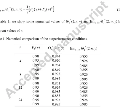
In Table 1, we show some numerical values of 1*(2,n,y) and lim (2, , )
*
1 y
n for
[image:15.612.111.516.235.596.2]different values of n.
Table 1. Numerical comparison of the outperformance conditions
n F2(y) *(2, , ) 1 n y
lim *(2, , )
1 n y
n
4
0.90 0.844 0.855
0.95 0.920 0.926
0.99 0.984 0.985
8
0.90 0.849 0.855
0.95 0.923 0.926
0.99 0.984 0.985
12
0.90 0.851 0.855
0.95 0.924 0.926
0.99 0.985 0.985
24
0.90 0.853 0.855
0.95 0.925 0.926
0.99 0.985 0.985
for low values of n and becomes very low for n12, with almost no difference (to the
third decimal place) for F2(y) = 0.99. This shows that for such demand histories, the
asymptotic condition is a very good approximation for assessing the comparative
performance of the two approaches.
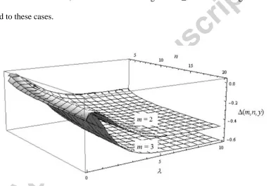
In Figure 1, we plot the variation of (m,n,y) with respect to the length of the demand
history n and the mean demand for y = 1 and for m = 2 and m = 3. To simplify the
presentation of the results, we do not show findings for m ≥ 4 but it is straightforward to
[image:16.612.117.502.270.535.2]extend to these cases.
Figure 1. The relative benefit of the OB approach for Poisson distributed demand
The results in Figure 1 show that the ratio (m,n,y) is negative in almost all cases,
which means that, under the Poisson assumption, the OB approach leads to a variance
reduction, which shows the outperformance of this approach. The results also show that,
for very low values of , i.e. slow moving demand, the relative benefit from using OB
instead of NOB is low when n is low. Moreover, there are very few values where the
relative benefit is positive, which correspond to cases where both
and n are very low. Figure 1 illustrates that the relative benefit stemming from the use of OB instead of NOBincreases substantially as the aggregation level m increases from 2 periods to 3 periods.
Further increases will follow as m increases to 4 periods or more.
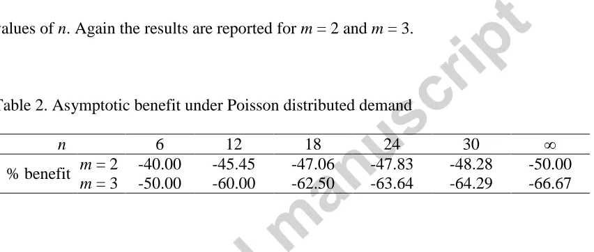
In Table 2, we show the benefit of using the OB approach as compared to the NOB for an
[image:17.612.95.521.239.420.2]infinite value of
(i.e. as an approximation for a very fast moving item) and different values of n. Again the results are reported for m = 2 and m = 3.Table 2. Asymptotic benefit under Poisson distributed demand
n 6 12 18 24 30 ∞
% benefit m = 2 -40.00 -45.45 -47.06 -47.83 -48.28 -50.00
m = 3 -50.00 -60.00 -62.50 -63.64 -64.29 -66.67
The numerical results in Table 2 show that for a very fast moving item, characterised by
Poisson distributed demand, the benefit of using the OB approach is very high varying
from 40% to 50% for m = 2 and from 50% to 66.7% for m = 3. Obviously, this benefit is
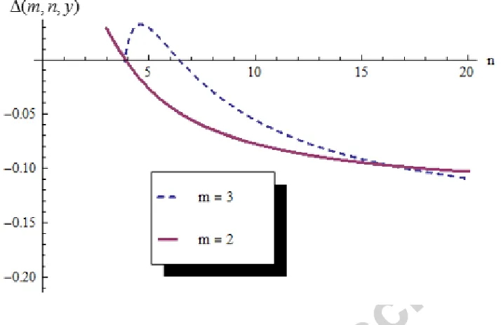
Figure 2. Relative benefit of using OB with respect to n when
= 0.5 and y = 1Figure 2 shows that for m = 2 and values of n4 (i.e. a very short demand history), the
NOB approach performs better than OB with a benefit varying between 0% and 3%.
Moreover, when m increases, (e.g. m = 3), the NOB approach performs better than OB
for values of n that can go up to 6. However, for higher values of n, OB outperforms
NOB and the benefit of using the former approach can go up to 11%.
In summary, the most interesting insights that could be provided based on the analysis of
the Poisson case are the following. With the exception of the context of short demand
histories’ length, overall the OB approach outperforms the NOB approach and the
relative benefit stemming from the use of OB increases substantially as the aggregation
level or the rate of the demand increases.
In this section, we discuss details related to our empirical investigation. First, we provide
information on the empirical data used in this research. Then, we present the
experimental structure employed, some simulation related details and the empirical
results.
5.1. Empirical data
For the purpose of our investigation, we use a dataset that comes from the US jewellery
industry. It contains the weekly demand history of 4,076 intermittent demand SKUs over
a period of one year (52 weeks). The lead time is fixed for all SKUs to one week.
Descriptive statistics are provided in Table 3. ‘Demand sizes’ refer to the sizes of demand,
when demand occurs, i.e. the relevant statistics refer only to demand occurring periods.
‘Demand intervals’ refer to the number of periods with zero demand plus one (for
example, if there are no zero demands between two periods with occurring demands, the
demand interval is one). ‘Demand per period’ refers to all periods, including both the
demand occurring and non-demand occurring ones. In order to illustrate the calculation
of demand sizes, demand intervals and demand per period, we consider the following
example with a demand history of 24 periods:
0 0 0 3 0 0 2 0 0 0 0 2 0 0 0 4 0 0 0 0 0 6 0 1
In this example, the demand sizes are 3, 2, 2, 4, 6 and 1 which provides an average
demand size of 3. Let us suppose that the period immediately preceding this history
contained a non-zero demand value. Then the demand intervals are equal to 4, 3, 5, 4, 6
These calculations are done per SKU in the dataset then averaged across SKUs to result
in the statistics shown in Table 3.
Table 3. Descriptive statistics of the empirical data
4,076 SKUs Demand Sizes Demand Intervals Demand per period Mean St. Deviation Mean St. Deviation Mean St. Deviation
Min 1.000 0.000 1.275 0.564 0.115 0.323
25%ile 1.100 0.316 3.286 2.629 0.192 0.445
Median 1.200 0.426 4.364 3.711 0.250 0.530
75%ile 1.353 0.651 5.625 5.046 0.365 0.673
Max 3.194 3.682 8.667 12.987 2.212 2.539
The descriptive statistics reported in Table 3 show that most of the SKUs are slow
moving since the distribution of demand intervals is mainly concentrated around a
median of 4.4 weeks, and most demands are for one or two units. It should also be noted
that the average minimum demand interval across SKUs is 1.3 (i.e. a value that is strictly
higher than 1) which means that for each SKU there are some zero demands between
demand occurrences. In the following subsections, we analyse the empirical performance
of both approaches. Firstly, variance reductions are assessed, and then the stock control
results are examined.
5.2. Statistical performance
We present the summary statistics of the variance ratio of the NOB approach to the OB
approach, Var
FˆmNOB(y)
/VarFˆmOB(y)
. Note that the calculation of the variances is performed by using the analytical results given in (2) and in Proposition 1 and byconsidering the entire demand history composed of 52 periods, which means that a
Table 4. Empirical comparative performance for long demand histories
m = 2 m = 3
Variance ratio for y=0
Variance ratio for y=1
Variance ratio for y=2
Variance ratio for y=0
Variance ratio for y=1
Variance ratio for y=2 Min 1.0214 1.0196 0.9953 1.0249 1.0289 0.9970
25% percentile 1.0392 1.1016 1.1244 1.0691 1.1225 1.1660
Median 1.0521 1.1332 1.4948 1.0941 1.1524 1.3429
Average 1.0662 1.1842 1.3853 1.1220 1.1721 1.3061
75% percentile 1.0806 1.1827 1.6292 1.1511 1.1854 1.4620
Max 1.4342 1.6308 1.7311 1.9506 1.5562 1.5274
The results in Table 4 show that, for a long demand history, the OB approach is expected
to outperform NOB for almost all the SKUs, with a median benefit, when y = 1, of 13%
for m = 2 and 15% for m = 3. Furthermore, when y = 2, the median benefit increases and
can go up to 49% for m = 2 and 34% for m = 3.
We now present the summary statistics of the variance ratio, Var
FˆmNOB(y)
/Var FˆmOB(y)
, for a length of the history n = 9. The calculation of the variances is no longer based on theanalytical results given in Proposition 1. Instead, it is performed by splitting the demand
history in five blocks composed of 10 periods (or 9 periods) when m = 2 (or m = 3), i.e.
the values of FˆmNOB(y) and FˆmOB(y) are first calculated for each block (by first
calculating the aggregated demands over the block and then deducing the probability that
the aggregated demand over the block is less or equal to y) and then their variances are
calculated by considering the 5 blocks. Note that in the former case, we consider a
demand history composed of 50 periods whereas in the latter, only 45 periods are
probabilities whereas a long length of blocks implies a low number of blocks which makes it
[image:22.612.95.525.164.324.2]difficult to calculate the variance of the estimates over the blocks.
Table 5. Empirical comparative performance for short demand histories
m = 2 m = 3
Variance ratio for y=0
Variance ratio for y=1
Variance ratio for y=2
Variance ratio for y=0
Variance ratio for y=1
Variance ratio for y=2
Min 0 0 0 0 0 0
25% percentile 0.7650 0.7088 0.7069 0.7259 0.7424 0.8167
Median 0.9504 0.9927 1.1270 0.9722 1.0889 1.3611
Average 1.0195 1.49284 1.52613 1.1534 1.6431 2.2713
75% percentile 1.1719 1.7357 1.7446 1.3199 1.8148 5.4444
Max 7.5600 16.2000 16.2000 9.0741 13.6111 13.6111
The results in Table 5 show that a high proportion (i.e. approximately 50%) of the SKUs
has a variance ratio less than 1, i.e. the NOB approach outperforms OB. These results,
showing performance superiority of the NOB approach for a short demand history, are
consistent with the theoretical results established earlier in this paper, which
demonstrated that such outperformance may arise in these circumstances. A more
detailed analysis was conducted but no link was established between the variance ratio
and the degree of intermittence (as characterised by the length of demand intervals). This
is not consistent with the analytical findings in Section 2.3, and the discrepancy would
seem to merit further empirical research on other datasets.
5.3. Stock control performance
In this subsection, we conduct an empirical comparison of the two approaches when an
Order-Up-To-Level (OUTL) inventory control policy is used. Under each approach, the
OUTL is calculated at the end of each period as the minimum number y such that Fˆm(y)
replenishment cycle), as shown in (15) and (16). We assume that unmet demand is
backordered.
F y CSL
CSL
SmNOB( )argminy ˆmNOB( ) (15)
F y CSL
CSL
SmOB( )argminy ˆmOB( ) (16)
In order to simulate the performance of each approach, we split the demand history
available (i.e. 52 periods) for each SKU into two parts. The 1st part (26 periods) is used in
order to initialise the inventory level (that is assumed to be equal to the initial OUTL).
The 2nd part (26 periods) is used for the out-of-sample generation of results and
evaluation of performance. In each part, n historical periods are considered to aggregate
the demand using one of the two approaches and then FˆmNOB(y) and FˆmOB(y)are
calculated in order to determine the OUTLs SNOB(CSL)
m and S (CSL)
OB
m . The initial values
of SmNOB(CSL)and S (CSL)
OB
m are calculated at the end of period 26 and then they are
updated in each period of the out-of-sample as described above. The order of events in a
period (i.e. a week) is as follows: the demand is first observed, the order (placed one
week ago) is received, and a new order is then placed. This dynamic simulation of the
inventory system uses an OUTL method calculated differently with the two aggregation
approaches. This enables us to calculate at the end of the demand history, the average
inventory holding volumes and backordering volumes, which allows a direct comparison
of the performance of the two approaches. We refer the reader to Syntetos and Boylan
We analyse the stock control results by assessing the trade-offs between the average
(across all SKUs) inventory holding volumes and the average backordering volumes.
This analysis is conducted for three target CSLs, namely CSL = 80%, 90%, 95%, three
demand history lengths, n = 6, 12, 24, and two aggregation levels, m = 2, 3.
We begin by presenting in Figures 3 and 4 the results for n = 24 in the form of efficiency
[image:24.612.114.502.243.710.2]curves for inventory holding and backordering volumes.
Figure 3. Efficiency curves for m = 2 and n = 24
0.02 0.03 0.04 0.05 0.06 0.07 0.08 0.09
0.90 1.10 1.30 1.50 1.70 1.90 2.10
B
ackorder
ed
vol
ume
s
Inventory holding volumes
NOB OB
0.01 0.02 0.02 0.03 0.03 0.04 0.04 0.05 0.05
1.40 1.60 1.80 2.00 2.20 2.40 2.60
Ba
ck
o
rder
ed
v
o
lum
es
Inventory holding volumes
NOB
Figure 4. Efficiency curves for m = 3 and n = 24
Figures 3 and 4 demonstrate overall better inventory performance of OB for the case of n
= 24. Moreover, the improvement in inventory performance is greater for m = 3 than m =
2. This is consistent with expectations from our theoretical results on variance reductions.
For the cases of n = 6 and n = 12, no benefits in inventory performance have been
identified. In some cases, it is not even possible to draw efficiency curves because of
insensitivity of the inventory holding volumes to the target service level. Insensitivity of
inventory holding volumes is due to all target service levels (80%, 90% and 95%) being
achieved at the same OUTL. Such a situation would not arise for faster moving SKUs but
is more prevalent for slow moving items. This problem is exacerbated for shorter demand
histories as there is less opportunity to smooth the CDF with fewer blocks.
6. Conclusions and future work
In this paper, based on a theoretical analysis, we have shown that the overlapping
aggregation approach produces unbiased estimates of the cumulative probability of
demand and we have established an expression for its variance, assuming identically and
independently distributed demand. Based on this analysis, we have established conditions
for the variance outperformance of the two approaches. Our analysis reveals that the
overlapping approach outperforms the non-overlapping one in most cases. The
We have also shown that the non-overlapping approach is better than the overlapping one
for 50% of the SKUs for a short demand history of length 9 or 10 periods.
When the stock control performance is analysed, the empirical investigation shows that
for a demand history of 24 periods, the overlapping approach reduces the inventory
backordering volumes, whilst maintaining the same inventory holding volumes. For
shorter demand histories, no benefit in inventory performance has been identified due to
the lack of opportunity to smooth the CDF with a small number of blocks.
The managerial implications of this research are clear if standard parametric distributions
are not appropriate and a non-parametric ‘temporal aggregation’ approach is adopted.
Unless the demand history is short, there is a clear advantage of using overlapping blocks
instead of the non-overlapping approach. The margin of this advantage becomes greater
for longer lead-times (equal to the length of the block). There are strong analytical
arguments to support these managerial implications, in terms of the variance of the
estimates of the cumulative distribution function. There is also empirical evidence to
demonstrate that these can be translated into stock-control benefits too. However, these
benefits should be checked, for example by a simulation exercise, as the evidence to
support stock-control improvements needs to be verified in a broader range of inventory
environments.
In the light of the above discussion, an interesting avenue for further research would be to
broaden the empirical analysis by evaluating more varied datasets, including faster
the issue of smoothing the CDF such as bootstrapping methods which randomly sample
non-contiguous time periods. Such methods have been suggested in the literature (e.g.
Willemain et al. (2000)) and it would be beneficial to analyse their theoretical properties
and empirical performance.
Appendix A. Proof of Proposition 1
We suppose that the observations are split into overlapping blocks of length m, namely
OB
k OB OB
B B
B1 , 2 ,...., where k nm1 and BiOB
Yi,Yi1,...,Yim1
fork i1,2,..., .
We define Zi as the sum of demand values over a block of length m, i.e.
m j
j i
i Y
Z
1
1
(A1)
We also define for any value of
y
the indicator function:
for
0
for 1 ) (
,
y Z
y Z Z
I
i i i
y (A2)
An estimate of Fm(y) using the overlapping approach is then:
( )
1 ) ( ˆ
1 ,
k
i
i y OB
m I Z
k y
F (A3)
The expectation of
F
ˆ
mOB(
y
)
is given by:
ˆ ( )
1 ( ) 1 ( ) ( )1 1
, F y F y
k Z
I k E y F
E m
k
i m k
i
i y OB
m
(A4)
By definition, the variance of the estimator
F
ˆ
mOB(
y
)
can be written as:
2
2) ( ˆ )
( ˆ )
(
ˆ y E F y E F y
F
V mOB mOB mOB (A5)
The first term may be written:
j i
j y i y j
i
i y OB
m EI Z I Z
k Z
I E k y
F
E ˆ ( ) 2 12 , ( ) 2 12 , ( ) , ( ) (A6)
By definition of the indicator function, we have:
I
,(
Z
)
2
E
I
, (
Z
)
F
(
y
)
E
y i
y i
m , (A7)which implies that:
( )
1 ( ) 1 ( ) 1 ( ) 11 2 2
2 ,
2 F y k F y
k y F k Z
I E
k m
k
i m j
i m j
i
i
y
. (A8)
We now calculate the term
j
i
j y i
y Z I Z
I E k
) ( )
( 1
, ,
2
. In this term, there are some
k i i m i j j y i y k i m i j m j i j y iy Z I Z F y EI Z I Z
I E 1 1 1 , , 1 1 2 ,
, ( ) ( ) 2 ( ) ( ) ( )
(A9) 2 1 2 1 1 2 ) ( 2 ) 1 )( ( ) ( ) ( )
(y F y i m k m k m F y
F m k i m k i m i j m
(A10)The term
k i i m i j j y i
y Z I Z
I E 1 1 1 ,
, ( ) ( ) may be re-expressed by a single summation
(across the diagonals, from the diagonal which is the one just next to the ‘main diagonal’
to the one which is (m-1) away from the ‘main diagonal’). Hence:
1 1 1 1 1 , , ( ) ( ) ( ) ( ) m s s k i i m i j j y iy Z I Z k m s y
I
E (A11)
where
y Y Y Y y Y Y Y Y Y Y Y y Y s m j j s m m m s m m s m s m s m Y p y 0 ... 0 ... 0 ... 0 2 1 1 1 1 1 1 1 2 1 2 ) ( ... ... )
( (A12)
Assembling the terms in (A8), (A10) and (A11) leads to:
y Y Y Y y Y Y Y Y Y Y Y y Y s m j j m s m m OB m m m m s m m s m s m s m Y p s m k k y F k m k m k y F k y F Var 0 ... 0 ... 0 ... 0 2 1 1 1 2 2 2 1 1 1 1 1 1 2 1 2 ) ( ... ... ) ( 2 ) ( 1 ) 1 )( ( ) ( 1 )] ( ˆ [ (A13)The relative benefit from using the OB approach instead of NOB, (m,n,y) is given by:
1 ( )
1) ( ) ( ) 1 ( ) 1 2 ( 2 ) ( 1 ) 1 ( ) 2 2 )( 1 2 ( ) 1 ( 1 ) , , ( 1 1 2 2
y F n m y F y m n s m n y F m n m n m n m n y n m m m s m s m (A14)It is clear that when
tends towards infinity,Fm(y) tends towards 0. This means thatwhen
tends towards infinity, (m,n,y)tends towards:1 ) ( ) ( lim ) 1 ( ) 1 2 ( 2 ) 1 ( 1 ) , , ( 1 1 2
n m y F y m n s m n m n y n m m s m s (A15)We now calculate
) ( ) ( lim y F y m s
where 1sm1.
1 1 1 1 2 2 1 3 1 1 1 1 1 2 1 2 1 ... 0 10 0 0
... 0 ... 0 ... 0 2 1 0
)
(
..
...
)
(
...
...
)
(
)
(
m m m m m s m m s m s m s m Y Y y Y m j j y Y Y y Y Y Y y Y Y Y y Y Y Y y Y Y Y y Y s m j j y Y m sY
p
Y
p
y
F
y
(A16)which can be written as:
1 1 1 1 2 2 1 3 1 1 1 1 1 2 1 2 1 ... 0 10 0 0
... 0 ... 0 ... 0 2 1 0 ) 2 (
!
..
...
!
...
...
)
(
)
(
m m j m m m s m m s m s m s m j Y Y y Y m j j Y y Y Y y Y Y Y y Y m Y Y y Y Y Y y Y Y Y y Y s m j j Y y Y s m m sY
e
Y
e
y
F
y
(A17)
1 1 1 1 2 2 1 3 1 1 1 1 1 2 1 2 1 ... 0 10 0 0
... 0 ... 0 ... 0 2 1 0 ) (
!
..
...
!
...
...
)
(
)
(
m m j m m m s m m s m s m s m j Y Y y Y m j j Y y Y Y y Y Y Y y Y Y Y y Y Y Y y Y Y Y y Y s m j j Y y Y s m m sY
Y
e
y
F
y
(A18) Since
1 1 1 1 2 2 1 3 1 1 1 1 1 2 1 2 1 ... 0 10 0 0
... 0 ... 0 ... 0 2 1 0 ! .. ... ! ... ... m m j m m m s m m s m s m s m j Y Y y Y m j j Y y Y Y y Y Y Y y Y Y Y y Y Y Y y Y Y Y y Y s m j j Y y Y Y Y
is bounded and
1
1sm it is clear that:
0
)
(
)
(
lim
y
F
y
m s
(A19)
Hence: 1
) 1 ( 1 ) 1 ( 1 ) , , ( lim m n m n n m m n y n m
(A20)
In addition, since: 1
) 1 ( 1 ) 1 ( 1 ) , , ( lim m n m n n m m n y n m
(A21)
Then m m n n m m m n m n y n
m n n
n 1 1 ) 1 1 ( 1 lim 1 ) 1 ( lim ) , , ( lim
lim (A22)
which ends the proof of Proposition 4. .
References
Babai M. Z., Ali M. M. and Nikolopoulos K. (2012). Impact of temporal aggregation on stock control performance of intermittent demand estimators: Empirical analysis,
OMEGA, 40 (6), 713-721.
Chen A. and Blue J. (2010). Performance analysis of demand planning approaches for aggregating, forecasting and disaggregating interrelated demands, International Journal of Production Economics, 128, 586–602.
Chen A., Hsu C. H., and Blue J. (2007). Demand planning approaches to aggregating and forecasting interrelated demands for safety stock and backup capacity planning,
International Journal of ProductionResearch, 45, 2269–2294.
Johnston F. R. and Boylan J. E. (1996). Forecasting for items with intermittent demand.
Journal of the Operational Research Society, 47, 113–121.
Kefeng, Xu., Philip T. E. (2003). Managing single echelon inventories through demand aggregation and the feasibility of a correlation matrix, Computers & Operations Research, 30 (2), 297–308.
Kourentzes N., Petropoulos F. and Trapero J. R. (2014). Improving forecasting by estimating time series structural components across multiple frequencies, International Journal of Forecasting, 30, 291–302.
Kourentzes, N., Petropoulos, F., (2015). Forecasting with multivariate temporal aggregation: The case of promotional modelling, International Journal of Production Economics, in press, doi.org/10.1016/j.ijpe.2015.09.011.
Mohammadipour M. and Boylan J. E. (2012). Forecast horizon aggregation in integer autoregressive moving average (INARMA) models, OMEGA, 40(6), 703-712.
Porras E. M. and Dekker R. (2008). An inventory control system for spare parts at a refinery: An empirical comparison of different reorder point methods, European Journal of Operational Research, 184, 101-132.
Rostami-Tabar B., Babai M. Z., Syntetos A., and Ducq Y. (2013). Demand forecasting by temporal aggregation, Naval Research Logistics, 60, 479–498.
Rostami-Tabar B., Babai M. Z., Syntetos A., and Ducq Y. (2014). A note on the forecast performance of temporal aggregation, Naval Research Logistics, 61, 489-500.
Rostami-Tabar, B., Babai, M. Z., Ducq, Y., Syntetos, A. (2015). Non-stationary Demand Forecasting by Cross-Sectional Aggregation, International Journal of Production Economics, 170, 297-309.
Strijbosch, L. W. G., Syntetos, A., Boylan, J. E., and Janssen, E. (2011). International Journal of Production Economics, 133 (1), 470-480.
Syntetos, A. A. (2014). Forecasting by temporal aggregation. Foresight, 34, 6-11.
Syntetos, A. A., Boylan, J. E., (2005). The accuracy of intermittent demand estimates,
International Journal of Forecasting, 21, 303–314.
Syntetos A. A. and Boylan J. E. (2006). On the stock-control performance of intermittent demand estimators, International Journal of Production Economics, 103, 36–47.
Syntetos A. A., Boylan J. E. and Croston J. D. (2005). On the categorization of demand patterns. Journal of the Operational Research Society, 56, 495–503.
Teunter, R., Syntetos, A. A. and Babai, M. Z., (2010). Determining Order-Up-To Levels under Periodic Review for Compound Binomial (Intermittent) demand, European Journal of Operational Research, 203, 619-624.
Willemain T. R., Smart C. N., Shocker J. H. and DeSautels P. A. (1994). Forecasting intermittent demand in manufacturing: a comparative evaluation of Croston’s method,
International Journal of Forecasting,10, 529–538.
Willemain, T. R., Smart, C. N., and Schwarz, H. F. (2004). A new approach to forecasting intermittent demand for service parts inventories, International Journal of Forecasting, 20, 375-387.
Williams T. M. (1984). Stock control with sporadic and slow moving demand, Journal of the Operational Research Society, 35, 939–948.