Uncertainty aware generative models for inferring document class prevalence

4575

Uncertainty-aware generative models for inferring document class

prevalence

Katherine A. KeithandBrendan O’Connor College of Information and Computer Sciences

University of Massachusetts Amherst {kkeith,brenocon}@cs.umass.edu

Abstract

Prevalence estimationis the task of inferring the relative frequency of classes of unlabeled examples in a group—for example, the pro-portion of a document collection with posi-tive sentiment. Previous work has focused on aggregating and adjusting discriminative in-dividual classifiers to obtain prevalence point estimates. But imperfect classifier accuracy ought to be reflected in uncertainty over the predicted prevalence for scientifically valid in-ference. In this work, we present (1) a genera-tive probabilistic modeling approach to preva-lence estimation, and (2) the construction and evaluation of prevalence confidence intervals; in particular, we demonstrate that an off-the-shelf discriminative classifier can be given a generative re-interpretation, by backing out an implicit individual-level likelihood function, which can be used to conduct fast and simple group-level Bayesian inference. Empirically, we demonstrate our approach provides better confidence interval coverage than an alterna-tive, and is dramatically more robust to shifts in the class prior between training and testing.1

1 Introduction

The goal of prevalence estimationis to infer the relative frequency of classesyiassociated with

un-labeled examples (e.g. documents) from a group,

xi ∈ D. For example, one might want to

es-timate the proportion of blogs with a positive sentiment towards a political candidate (Hopkins and King, 2010), sentiment of responses to nat-ural disasters on social media (Mandel et al.,

2012), or prevalence of car types in street pho-tos to infer neighborhood demographics (Gebru et al., 2017). Often, an analyst wants to com-pare prevalence between multiple groups, such

1_{Code available at http://slanglab.cs.umass.}

edu/doc_prevalenceandhttps://github.com/ slanglab/doc_prevalence.

as inferring prevalence variation over time (e.g., changes to online abuse content (Bissias et al.,

2016)), or across other covariates (e.g., changes in police officers’ “respect” when speaking to mi-norities (Voigt et al., 2017)). This problem has been re-introduced in many different fields: as “quantification” in data mining (Forman, 2005,

2008), “prevalence estimation” in statistics and epidemiology (Gart and Buck, 1966), and “class prior estimation” in machine learning (Vucetic and Obradovic, 2001; Saerens et al., 2002). In NLP, SemEval 2016 and 2017 included Twitter senti-ment class prevalence tasks (Nakov et al., 2016;

Rosenthal et al.,2017).

Prevalence estimation assumes access to a (po-tentially small) set of labeled examples to train a classifier; but unlike the task of individual classi-fication, the goal is to estimate the proportion of a class among examples in a group. If a perfectly accurate classifier is available, it is trivial to con-struct a perfect prevalence estimate by counting the classification decisions (_§3.1). In fact, most application papers in the previous paragraph use this or a similar aggregation rule to conduct their prevalence estimates. However, classifiers often exhibit errors from different sources, including:

• Shifts in the class distribution from training to testing (Ptrain(y)6=Ptest(y)). A classifier

may be biased toward predictingPtrain(y).

• Difficult classification tasks (such as predict-ing sentiment or sarcasm) that result in low accuracy classifiers; this can be exacerbated by limited training data, as is common in so-cial science or industry settings that require manual human annotation for labels.

preva-lence estimates.2 However, there is relatively lit-tle understanding to what extent the quality of the document-level model impacts prevalence es-timates. Imperfect classifier accuracy ought to be reflected in uncertainty over the predicted preva-lence.

In this work, we tackle both of these challenges simultaneously, using a generative probabilistic modeling approach to prevalence estimation. This model directly parameterizes and conducts infer-ence for the unknown prevalinfer-ence, naturally ac-commodating shifts between training and testing, and also allows us to infer confidence intervals for the prevalence. We show that our best model can be seen as an implicit likelihood generative re-interpretation of an off-the-shelf discriminative classifier (§4.2); this unifies it with previous work, and also is easy for a practitioner to apply.

We additionally review several types of class prevalence estimators from the literature (§3), and conduct a robust empirical evaluation on senti-ment analysis over hundreds of docusenti-ment groups, illustrating the methods’ biases and robustness to class prior shift between training and testing. Our method provides better confidence interval cover-age and is more robust to class prior shift than pre-vious methods, and is substantially more accurate than an algorithm in widespread use in political science.

2 Problem definition

We consider two prevalence estimation problems: (1) point prediction and (2) confidence interval prediction. In this work, we are most interested in supervised learning for discrete-valued document labels, with access to a small to moderate number (e.g. around 1000) of labeled documents with text

x and labely: (xi, yi) ∈ Dtrain. We restrict

at-tention to binary-valued labelsy _{∈ {}0,1_}. At test time, there are one or more groups of unlabeled test documents,D(1)_{,· · · ,D}(G)_{; for example, one}

group might be a set of tweets sent during a cer-tain month, or a set of online reviews associated with a particular product. For each group D, let

θ∗ _≡(1/n)Pn

i yibe the true proportion of

posi-tive labels (wheren=_|D|).

The prevalence point prediction problem is to take an unlabeled document group_Das input and

2_{For example,Bissias et al.find a relative mean absolute}

error of less than 0.01 when the individual classifier has ROC AUC of 0.91.

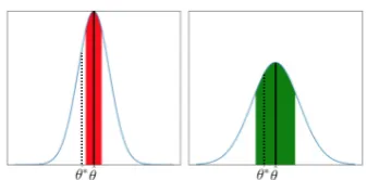
Figure 1: Example posterior distributions with MAP prevalence estimates, θˆ(solid line) and the true prevalence, θ∗ (dashed line). A desirable property is that confidence intervals, technically Bayesian credible intervals, (shaded regions) will be wider for more uncertain models. For exam-ple, the wider CI on the right (green) containsθ∗ whereas the narrower CI interval on the left (red) does not.

infer an estimated θˆ ∈ [0,1]. Ideally, this point estimate should be close to the true prevalenceθ∗; we evaluate this by mean absolute error.

In this work, we are the first (that we know of) to introduce the question ofuncertaintyin preva-lence estimation. Since document classifiers are typically far from perfectly accurate, we should expect substantial error in prevalence prediction, and inference methods should quantify such un-certainty. We formalize this as aprevalence con-fidence interval(CI) inference, which takes as in-put a desired nominal coverage level(1₋α), and predicts a real-valued interval [ˆθlo,θˆhi] ⊆ [0,1].

Ideally, a CI prediction algorithm should have fre-quentist coverage semantics: over a large number of test groups,3(1−α)%of the predicted intervals ought to contain the true valueθ∗. If the problem is hard—for example, the relationship between doc-ument features and the label is not captured well by the model—the CI should be wide. We em-pirically evaluate coverage of CI-aware prevalence inference models. See Fig.1for an intuitive exam-ple.

3 Review and baselines: Discriminative individual classification aggregation

The most straightforward baseline approach to prevalence estimation is to build on discrimina-tive, supervised learning for individual-level la-bels, such as binary logistic regression with bag-of-words features, randomized feature hashing

3_{Or in fact, across many experiments in which the model}

(Weinberger et al., 2009), or neural networks (Goldberg,2016). Such a model defines an indi-vidual document’s label probabilitypi ≡pβ(yi = 1 _|xi)where parametersβ are fit by maximizing

regularized likelihood on the labeled training data.

3.1 Classify and Count (CC)

For prevalence point estimation, Forman (2005) defines the “classify and count” (CC) method as simply averaging the most-likely individual label predictions,

ˆ

θCC = 1 n

X

i

1{pi >0.5}. (1)

This is the most obvious approach for practition-ers, but it has at least two weaknesses, which have been addressed in different groups of prior work. First, the class proportions may change be-tween training and test groups, which the Adjusted CC and ReadMe algorithms attempt to fix (_§3.2–

3.3). Second, it discards probabilistic informa-tion, which is remedied by the Probabilistic CC method, and an extension we propose (_§3.4–3.5).

3.2 Adjusted Classify and Count (ACC)

CC may encounter problems if the test class dis-tribution is different than the training’s. The “adjusted classify-and-count” method (Gart and Buck, 1966; Forman, 2005) treats the classifier output as a proxy variable, and estimates a sep-arate confusion model of classifier output yˆi ≡ 1_{pi>0.5}conditional on the true label,p(ˆy|y),

from cross-validation within the training set. As-suming the confusion model extends to the test data, a moment-matching approach is then used to infer the true label proportions, by first observing

ptest(ˆy) = P_yp(ˆy | y)ptest(y) and solving the

linear system for ptest(y), the test-time expected

class prevalence. Using empirical estimates for the true positive rate TPR = p(ˆy = 1 | y = 1), and false positive rate FPR = p(ˆy = 1_| y = 0), and

ˆ

θCC _{=p(ˆy= 1), it has the closed form}

ˆ

θACC = θˆ

CC_−FPR

TPR₋FPR. (2)

By design, ACC is more robust to a new test-time prevalence, but it relies on the accuracy of its TPR and FPR estimates, and its lack of probabilistic se-mantics makes it unclear how to infer confidence intervals.

3.3 ReadMe algorithm

An interesting extension to ACC is to remove the need for a discriminative classifier, by directly modeling text conditional on the latent document class. The ReadMe algorithm, developed in po-litical science (Hopkins and King,2010), extends ACC’s linear system for every term type in a (subsampled and augmented) term vocabularyV, and calculates their class-conditional probabilities from the training data. Assuming these condi-tional models also hold in the test data, that im-pliesptest(w) = P_yp(wˆ | y)ptest(y); the

algo-rithm infers ptest(y) by minimizing the squared

error of predicted versus empirical term frequen-cies in the test set. The open-source ReadMe soft-ware package4 has been used in numerous politi-cal science studies, including inferring proportions of types of censored Chinese news (King et al.,

2013), credit claiming in Congressional press re-leases (Grimmer et al.,2012), and voter intentions among Twitter messages (Ceron et al.,2015).

ReadMe is theoretically appealing in that it infers latent class prevalences to explain the test group’s textual evidence; but as a non-probabilistic model, it does not directly imply a method for confidence intervals (Hopkins and Kinguse the bootstrap). Furthermore, our experi-ments (§5), contra the original paper, show its im-plementation exhibits poor performance.

3.4 Probabilistic Classify and Count (PCC)

Both the CC and ACC methods discard uncer-tainty information from the classification model. In a difficult classification setting, for example, we might expect many probabilities to be near, say,

0.6, in which case the CC method may undercount the negative class. This suggests an alternative method, “probabilistic classify and count” (PCC):

ˆ

θP CC = 1 n

X

i

pi (3)

which is the expected prevalence,(1/n)P iyi,

as-suming eachyiis distributed according to the

orig-inal probabilistic classifier.

3.5 PCC Poisson-Binomial distribution (PB-PCC)

If we assume each yi is conditionally

indepen-dent given text xi and model parameters β, this

defines a fully probabilistic model for the class prevalence. Let the latent variableS =P

iyi; its

distribution is thus Poisson-Binomial (Chen and Liu,1997). The modeled prevalence distribution

p(S_n | D)can be exactly inferred by Monte Carlo inference: each iteration samples every yi and

sums for anS sample. TheS/ndistribution over many iterations can be used to construct a Monte Carlo CDFFˆ, from which any[ ˆF(t),Fˆ(t+1₋α)]

is an(1₋α)-sized credible interval (where0 _≤ t ≤ t+ 1−α ≤ 1). This model has prevalence expectationE[S_n] = ˆθP CC_{, and variance}

Var

S n

= 1 n2

X

i

pi(1−pi). (4)

To a certain degree, this model captures uncer-tainty in the classifier since per-document vari-ance, pi(1−pi), is high whenpi = 0.5and low

when near 0 or 1. However, it also has a major weakness—the variance concentrates with a large test group size n, which is the wrong behavior when a classifier is truly noisy, for example, when a classifier is genuinely uncertain and predicts the same constantpi = q for each document. In this

case, the correct behavior would be to maintain a flat, wide posterior belief aboutθ, which is better accomplished by the generative model we intro-duce in the subsequent section.

4 Our approach: generative probabilistic modeling

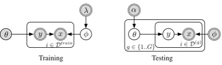
We turn to generative modeling, that seeks to to jointly model the probability of labels and text in both the training and test groups, by assum-ing a document’s text is generated conditional on the document label. Language models have widespread use in natural language processing, and class-conditional models have been used for document classification (e.g. multinomial Naive Bayes;McCallum and Nigam(1998)). We use a similar generative setup to explicitly model a class prevalence for test groupg, with a generative story for each (bag-of-words) documentiin the group:

θg ∼Dist(α) (5)

yi,g ∼Bernoulli(θg) (6) xi,g ∼Multinomial(φyi,g) (7)

The test group is assumed to have a latent class priorθg, which itself has a prior distribution (we

assume Dist(α) = Unif(0,1)in this work). For

✓ y x

g2 {1..G} i2 D(g)

✓ y x

i2 Dtrain

↵

Training Testing

Figure 2: Our generative model for prevalence esti-mation. Left: Class-conditional language models (φ) are learned at training time. Right: Test-time inference for multiple groups’ latent prevalences (θ).

each classk,φkis a class-conditional unigram

lan-guage model, which is learned from the training data but fixed at test time. We then perform infer-ence to findθgthat gives a high probability to text

data{xi ∈ D(g)}. Figure2shows the probabilistic

graphical model.

4.1 MNB and Loglin language models

We experiment with two explicit language mod-els in this generative framework: (1) multinomial Naive Bayes (MNB), using a training-time sym-metric Dirichlet prior φy ∼ Dir(λ/V) for

vo-cabulary sizeV and “pseudocount”λ, and (2) an additive log linear model (Loglin, a.k.a. SAGE (Eisenstein et al.,2011)). Loglin estimates words’ probabilities as deviations from a background log-probabilitym,

ηy,w∼Laplace(λ) (8)

φy,w= exp(mw+ηy,w)/ X

j

exp(mj+ηy,j)

where mw is the empirical log probability of

a word w among all training documents, and

ηy,w denotes class-specific deviations of the

log-probability of a word w, MAP estimated under a sparsity-inducing L1 penalty. Such sparse ad-ditive models have been used in both supervised and unsupervised document modeling; for exam-ple, as a document-level posterior classifier it out-performs MNB (Eisenstein et al.,2011), or even discriminative models (Taddy,2013), and its spar-sity helps interpretability for analyzing political, literary, and legal texts (Monroe et al.,2008;Sim et al., 2013; Bamman et al., 2014; Wang et al.,

2012).

4.2 Implicit likelihoods from discriminative classifiers (LR-Implicit)

models because it sets up a likelihood and pos-terior distribution over θ. But in terms of docu-ment modeling for classification purposes, the in-dependence assumptions of the generative model are typically too strong, and for document-level classification, discriminative models tend to out-perform similarly parameterized generative ones, especially when the training set is sufficiently large (Ng and Jordan, 2002). Thus, discrimina-tive models may have information better suited to class prevalence inference. Also, since the most common practice for document classification is to use discriminative models, it would be helpful to more effectively use discriminative posteriors within our generative context.

In Naive Bayes-style generative document clas-sification, the model definespgen(x |y)and class

prior p(y), which are combined to calculate the posterior pgen(y | x) ∝ pgen(x | y)p(y).

Dis-criminative models, by contrast, directly define a

pdisc(y |x). We can, however, expand this

quan-tity via Bayes Rule:

pdisc(y|x) =pimplicit0(x|y)ptrain(y)/p(x). (9)

The “implicit document likelihood” p_implicit0(x |

y)is a likelihood function that, combined with a particular class prior p(y), would have resulted in the same posterior predicted by the discrim-inative model. Given the discriminative poste-rior predictions and the training-time class pposte-rior

ptrain(y) = ˆθtrain, an implicit likelihood function

can be backed out for any particular documentx; we define the “simple implicit” likelihood for doc-umentxto be:

pimplicit(x|y) =pdisc(y|x)/θˆtrain. (10)

This takes the form of a correction of the discrim-inative posterior, by dividing out the training-time class prevalence.5

Our LR-Implicit generative model uses the same class prevalence and document label genera-tion setup as before, but to calculate the individual documents’p(x _| y) probabilities, it usespimplicit

based on a logistic regressionpdisc.6

5_{Technically,p}

implicit0 is retrievable only up to a constant,

andpimplicitis one particular compatible implicit likelihood,

since it can be multiplied by any constant and is still consis-tent with Eq.9, and would give rise to the same document-and group-level posteriors.

6_{The implicit likelihood still has the form of a}

logis-tic regression, adjusting its bias term: if pdisc(y | x) =

σ(β0x + β0), then pimplicit(x | y) = σ(β0x + β0 −

log (θtrain/(1−θtrain))).

This model is inspired bySaerens et al.(2002)’s EM algorithm for adjusting a classifier for a test set’s class prior; they derive it differently by ap-plying the assumptionptrain(x |y) =ptest(x |y),

expanding each side with Bayes’ Rule, solving for

ptest(y | x), then estimatingptest(y)via EM. This

in fact optimizes the same marginal likelihood function in the next section under the implicit-discriminative generative model; our formulation broadens it as a fully Bayesian or likelihood-based model.

4.3 Inference

To estimate class prevalence, we use the marginal log likelihood overθto obtain a posterior overθ. For each each test groupg, we have the marginal log probability of all document texts,

MLLg(θ)≡logp(D(g)|θ) (11)

= X

i∈D(g)

log X y∈{0,1}

p(xi, yi =y|θ)

= X

i∈D(g) log

θL+_i + (1−θ)L−_i

,

where we denote the class-conditional document text likelihoods L+_{i ≡} p(xi | yi = 1) and L−_i ≡p(xi|yi= 0). The gradient for an

individ-ual document is(L+_{i −}L−_i )/(θL+_i + (1₋θ)L−_i ); intuitively, the sign of the numerator says that documents that are more likely under the positive than negative class encourage higher likelihood for larger values ofθ. When the model is uncertain about a document—that is, whenL+_i ≈L−_i —that document contributes a relatively flat likelihood curve, expressing little preference for likely val-ues ofθ. If a model is more heavily regularized— for example, when the log-linear additive model is more dominated by the background language model—this condition tends to hold for the doc-uments, leading to a flat, highly uncertain likeli-hood curve.

The marginal log likelihood is unimodal over

θ∈[0,1], since it is concave, being a sum of con-cave log-linear functions, and having negative cur-vature:

∂2_MLL g

∂θ2 =−

X

i∈D(g)

L+ i −L

−

i θL+_i + (1₋θ)L−_i

2 .

(12)

used to reliably find a mode, including EM or first-or second-first-order methods. At least two approaches to inferring confidence intervals are possible. One is to use a central limit theorem-style approxima-tion, assuming the sampling distribution is approx-imated by a normal with meanθMLE_{and variance}

−[∂2_MLL

g/∂θ2]−1. The second, which we focus

on, is Bayesian estimation forlogp(θg | D(g)) ∝ logp(θg) + MLLg(θg) by simply using a grid

search over valuesθ_{∈ {}0.001,0.002, ...0.999_}to infer both the posterior mode θMAP _{as well as a}

90% highest posterior density interval.7 In small-scale experiments, this model had very similar re-sults to the central limit theorem (with EM for

θMLE_).

5 Experiments

5.1 Data

In order to compare document class prevalence estimators, we desire datasets that (1) have natu-ral document groups that correspond to realistic, real-world applications, (2) have a large number of test groups (hundreds or more), and (3) are freely available for academic research. It has been a challenge to fulfill these criteria in previous work.

Nakov et al. (2016) conduct large-scale manual annotation of Twitter sentiment for SemEval 2016 Task 4, with topic-based test groups; unfortu-nately, redistribution is restricted to message IDs, making the original dataset difficult to reconstruct under Twitter’s terms of service if messages have since been deleted. Bella et al. (2010) andEsuli and Sebastiani (2015) use large, pre-existing la-beled document corpora, but they do not contain natural groups; evaluations utilize randomly sam-pled synthetic groups.

To better fulfill these criteria, we select the task of business review sentiment prevalence, where the goal is to estimate the proportion of reviews that are positive for one particular business; specif-ically, we use labeled data from the Yelp Dataset Challenge Round Nine8corpus, which consists of 4.1M reviews by 1M users for 144K businesses. We sample 500 businesses with at least 200 re-views each as the test groups. We treat the task as binary classification, and assignyi = 1to reviews

7_{Since we use a uniform prior, this is just the MLE.}

Tech-nically, we used a prior of Beta(1.0001,1.0001)to avoid cer-tain issues with tie-breaking, but it was not necessary.

8_{Downloaded June 2017 fromhttps://www.yelp.}

com/dataset_challenge.

with 3 or more stars. This task seems reason-ably representative of real-world sentiment anal-ysis problems, and this type of dataset can easily be collected and reproduced from Yelp or other widely available review data.

For training, we simulate a small-scale annota-tion project by sampling 2000 labeled documents from the rest of the corpus. This is a natural prevalence that on average is about the same as the test groups, though individual test groups may have a much different prevalence (ranging from

0.096to0.997, mean (stdev) 0.823(0.136)). We also construct a synthetictraining setting with a highly skewed class prior, selecting 2000 docu-ments with a0.1 class prevalence (i.e. 200 posi-tive documents in the group). In each case, for ev-ery model, we re-run and average results over 10 different samples of the training set. For prepro-cessing, we tokenize with NLTK9and lowercase.

5.2 Model training

We use L1 regularization for logistic regression based on the vector of a documents’ word counts, to be most directly comparable to the generative models; for each model, we select its hyperparam-eter (LR and Loglin’sλ, or MNB’s pseudocount) by minimizing cross-validated cross-entropy of in-dividual document posteriors (within the labeled training set), over a grid search of powers of 2. The log-linear additive model is trained with OWL-QN (Andrew and Gao,2007)10and the logistic regres-sion model is trained with the default implementa-tion in scikit-learn (Pedregosa et al.,2011).11 We used ReadMe with its default parameters.12

5.3 Results

For each of the 500 test groups, we calculate a prevalence point estimateθˆwith each method, and evaluate by averaging across groups for mean ab-solute errorP

g|θˆg−θg∗|and bias P

g(ˆθg−θ∗g).13

For the models that allow for confidence interval

9_{http://www.nltk.org/} 10

Viagithub.com/larsmans/pylbfgs

11

Version 0.18.2

12_{Version 0.99837 fromhttps://gking.harvard.}

edu/readme, with default parameters features=15, n.subset=300, prob.wt=1. We bypass the ReadMe software’s text preprocessing pipeline, and instead have it use nearly the same document-term matrices as the other models. Since it only handles binary document-term matrices, we transformed counts to indicators; with other models this change only made a minor difference in results.

13_{For the generative (MLL) models,θˆis the MAP estimate;}

Natural training prevalence≈0.8 Synthetic training prevalence = 0.1

Point est. CIs Point est. CIs MAE Bias Cover. Width MAE Bias Cover. Width

Const. Pred. train mean 0.114 -0.045 — — 0.723 -0.723 — — Pred. 100% 0.177 0.177 — — 0.177 0.177 — —

ReadMe 0.233 -0.222 — — 0.383 -0.382 — —

Disc. (LR)

CC 0.048 0.042 — — 0.503 -0.503 — —

ACC 0.048 -0.001 — — 0.132 -0.015 — —

PB-PCC 0.049 -0.017 0.283 0.044 0.464 -0.464 0.001 0.054

Gen. (MLL)

MNB 0.078 0.058 0.120 0.046 0.199 -0.199 0.022 0.073 Loglin 0.089 -0.070 0.410 0.100 0.140 -0.036 0.510 0.273 LR-Implicit 0.050 0.001 0.454 0.074 0.069 -0.051 0.439 0.082

Table 1: Mean absolute error (MAE), bias, nominal 90% confidence interval coverage, and average CI width for the 500 Yelp data test groups, averaged over 10 simulations of resampled training (2000 doc-ument) sets. We examine both the natural positive class training prevalence (E[θtrain] =0.7783), and a

synthetic fixed prevalence of 0.1. Dashes indicate the methods that are not able to calculate confidence intervals.

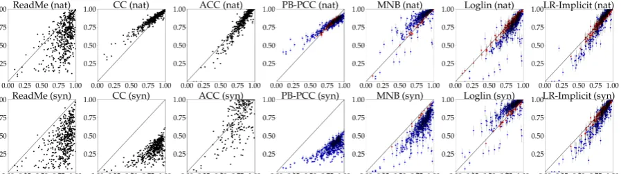
Figure 3: Gold prevalence θ∗ (x-axis) versus predicted prevalence θˆ(y-axis) for each of the 500 test groups with natural (nat) training prevalence (top row) and synthetic (syn) 0.1 training prevalence (bottom row). A blacky =xline is plotted for visualization. For the models that allow for confidence intervals, 90% CIs for each group are given by the faint grey lines. Blue dots indicate the CI does not containθ∗ and red dots indicate the CI does contain θ∗. For each setting, we show the the model with median MAE across training resamplings.

prediction, we infer 90% intervals and calculate coverage, which is best if it is 0.90. We also re-port average CI width; a narrower interval indi-cates more confidence (even if misplaced). Re-sults are in Table1; every result is averaged over 10 resamplings of the training set.

The ReadMe software did not have competitive performance; we hope in follow-up work to under-stand whyHopkins and Kingfound it had consid-erably stronger performance than SVM-based CC.

For the natural training class prevalence setting (first column, Table 1), the discriminative-based models (CC, PCC and the adjusted variants ACC and LR-Implicit) all have very similar point esti-mate performance, outperforming the purely

gen-erative models (MNB and Loglin). For CI cov-erage, the log-linear and LR-Implicit generative models have significantly better coverage than the discriminative model (PB-PCC) or MNB. Future work is required to improve coverage to be closer to the nominal ideal of 90%.

Figure 4: CI coverage rate (left two graphs) and average CI width (right two graphs) for three bins of the test groups, binned by number of documents.

(a) Varying training prevalence

(b) Varying training size

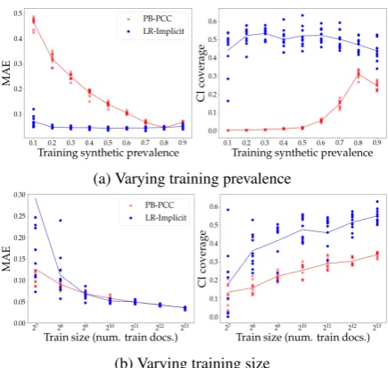
Figure 5: MAE and 90% CI coverage for PB-PCC while varying(a)training prevalence (the propor-tion of the 2000 training documents with positive reviews) and (b) training size (number of doc-uments in the training data) with natural preva-lence. Lines are the averages over 10 resamplings of training sets and points represent one resam-pling.

consistently strong performance in both training settings, and for both point estimation and (rela-tively, at leas) confidence intervals.

Figure3showsθ∗ _{versusθˆfor each of the 500} test groups for each of the models, including pre-dicted CIs. CC’s and PCC’s erroneous assump-tions are directly viewable: in the natural preva-lence setting, the slope shallower than 1, indicat-ing a persistent under-sensitivity to the true class prevalence—unlike ACC and the generative mod-els. In the synthetic training case, CC and PCC wildly underpredict, presumably because they are biased by the low training-time prevalenceθtrain =

0.1.

5.4 Comparison of PB-PCC and LR-Implicit

Since PB-PCC and LR-Implicit represent the strongest members of non-adjusted classification aggregation and generative modeling, respec-tively, we further compare their results. When varying synthetic training prevalence across 0.1 to 0.9 (Figure5a), LR-Implicit has much better MAE in all settings except near the natural prevalence (the test groups have, on average, 0.82 positive prevalence), and consistently stronger CI cover-age.

Figure5bshows results for natural class preva-lence when varying the training set size. Unfortu-nately, LR-Implicit is disadvantaged at very small test sizes—its MAE is higher when there are only a few hundred training documents (≤28 _{= 256),}

though performance converges after that. We sus-pect this may occur because, when textual evi-dence is weak, the classifier learns to more heavily rely on its bias term, which can be a useful form of bias when the training class prevalence matches the test groups (on average). However, at all lev-els, LR-Implicit’s coverage is better.

Since we hypothesized that PB-PCC may be overconfident for large test groups (§3.5), we test this by binning test groups by the number of doc-uments per group. Figure4confirms that PB-PCC exhibits overconfidence for larger groups (smaller CI width alongside lower CI coverage), but LR-Implicit suffers from the same problem as well.

6 Additional Related Work

article topics (RCV1) and medical record subject heading (OHSUMED-S) class prevalence tasks, finding varying results among CC, ACC, and PCC. A number of other empirical evaluations were con-ducted in two SemEval Twitter sentiment preva-lence shared tasks, with varying results among these and other methods with a range of classifiers (Nakov et al.,2016;Rosenthal et al.,2017);Nakov et al. note that CC was often one of the strongest methods. Esuli and Sebastiani as well as Xue and Weiss (2009) present semi-supervised loss-augmented classifier training methods to improve prevalence estimation.Tasche(2017) presents the-oretical results for ACC and Saerens et al.’s EM method (what we call the LR-Implicit MLE), ar-guing they correctly predict θ∗ _{under class prior} shift; we confirm that those two methods are in-deed better than many alternatives in our empir-ical evaluation. While we focus on inference of the test-time class prior as a class prevalence esti-mate,Saerens et al.(2002) also show their method can improve individual-level classification accu-racy, which Sulc and Matas (2018) use for im-age classification. (From the viewpoint of indi-vidual classification, this phenomenon is known as prior probability shift (Moreno-Torres et al.,

2012).) Gonz´alez et al. (2017b) and Card and Smith (2018), similarly to our results, find that CC is much poorer than ACC under class shift.

Card and Smithalso show that PCC can be sensi-tive to properties of the classifier, finding that well-calibrated classifiers can give strong performance. They argue that discriminative aggregation models are appropriate for tasks where humans respond to text. Jerzak et al. (2018) analyze issues in class prevalence estimation and propose the ReadMe2 algorithm, which adds external word embeddings, optimization-based dimension reduction, and sim-ilarity matching to ReadMe’s moment-matching framework.

7 Conclusion

Document class prevalence estimation is a widespread and much understudied task. We show that simple and obvious classifier aggrega-tion methods display consistent biases, especially under class prior shift. Given how widely some of the less effective methods are used, machine learning and natural language processing research could have real impact in this space.

We also call attention to the need for

uncer-tainty aware inference—methods that give con-fidence intervals to summarize their uncertainty. While our method is a first step, future work is necessary to better understand the problem and develop methods with improved coverage. Also, our framework can accommodate a wide array of document and language models—while we fo-cus on bag-of-words models, recent advances in sequence, neural, and attention-based document models could be added directly to our generative model, or used as a discriminative-implicit com-ponent. The overall framework could also be ex-tended to multiclass, and potentially, structured prediction settings.

References

Galen Andrew and Jianfeng Gao. 2007. Scalable train-ing of L1-regularized log-linear models. In Pro-ceedings of the 24th International Conference on Machine Learning.

David Bamman, Ted Underwood, and Noah A. Smith. 2014. A Bayesian mixed effects model of literary character. InProceedings of the 52nd Annual Meet-ing of the Association for Computational LMeet-inguis- Linguis-tics.

Antonio Bella, Cesar Ferri, Jos´e Hern´andez-Orallo, and Maria Jose Ramirez-Quintana. 2010. Quantifi-cation via probability estimators. InIEEE 10th In-ternational Conference on Data Mining (ICDM).

George Bissias, Brian Levine, Marc Liberatore, Brian Lynn, Juston Moore, Hanna Wallach, and Janis Wolak. 2016. Characterization of contact offend-ers and child exploitation material trafficking on five peer-to-peer networks. Child Abuse & Neglect, 52:185 – 199.

Dallas Card and Noah A Smith. 2018. The importance of calibration for estimating proportions from an-notations. InProceedings of Empirical Methods in Natural Language Processing.

Andrea Ceron, Luigi Curini, and Stefano M Iacus. 2015. Using sentiment analysis to monitor elec-toral campaigns: Method matters—evidence from the United States and Italy. Social Science Com-puter Review, 33(1):3–20.

Sean X. Chen and Jun S. Liu. 1997. Statistical ap-plications of the Poisson-binomial and conditional Bernoulli distributions. Statistica Sinica, pages 875–892.

Andrea Esuli and Fabrizio Sebastiani. 2015. Optimiz-ing text quantifiers for multivariate loss functions. ACM Transactions on Knowledge Discovery from Data (TKDD), 9(4):27.

George Forman. 2005. Counting positives accurately despite inaccurate classification. InEuropean Con-ference on Machine Learning.

George Forman. 2008. Quantifying counts and costs via classification. Data Mining and Knowledge Dis-covery, 17(2):164–206.

John J. Gart and Alfred A. Buck. 1966. Comparison of a screening test and a reference test in epidemiologic studies. II. A probabilistic model for the comparison of diagnostic tests. American Journal of Epidemiol-ogy, 83(3):593–602.

Timnit Gebru, Jonathan Krause, Yilun Wang, Duyun Chen, Jia Deng, Erez Lieberman Aiden, and Li Fei-Fei. 2017. Using deep learning and Google Street View to estimate the demographic makeup of neigh-borhoods across the United States. Proceedings of the National Academy of Sciences.

Yoav Goldberg. 2016. A primer on neural network models for natural language processing. Journal of Artificial Intelligence Research, 57:345–420.

Pablo Gonz´alez, Alberto Casta˜no, Nitesh V. Chawla, and Juan Jos´e Del Coz. 2017a. A review on quantification learning. ACM Computing Surveys, 50(5):74:1–74:40.

Pablo Gonz´alez, Jorge D´ıez, Nitesh Chawla, and Juan Jos´e del Coz. 2017b. Why is quantification an interesting learning problem? Progress in Artificial Intelligence, 6(1):53–58.

Justin Grimmer, Solomon Messing, and Sean J West-wood. 2012. How words and money cultivate a per-sonal vote: The effect of legislator credit claiming on constituent credit allocation. American Political Science Review, 106(4):703–719.

Daniel J. Hopkins and Gary King. 2010. A method of automated nonparametric content analysis for so-cial science. American Journal of Political Science, 54(1):229–247.

Connor T. Jerzak, Gary King, and Anton Strezhnev. 2018. An improved method of automated nonpara-metric content analysis for social science. Working paper.

Gary King, Jennifer Pan, and Margaret E Roberts. 2013. How censorship in china allows government criticism but silences collective expression. Ameri-can Political Science Review, 107(2):326–343.

Benjamin Mandel, Aron Culotta, John Boulahanis, Danielle Stark, Bonnie Lewis, and Jeremy Rodrigue. 2012. A demographic analysis of online sentiment during Hurricane Irene. InProceedings of the Sec-ond Workshop on Language in Social Media, pages 27–36. Association for Computational Linguistics.

Andrew McCallum and Kamal Nigam. 1998. A com-parison of event models for naive Bayes text classi-fication. InAAAI-98 Workshop on Learning for Text Categorization.

Burt L. Monroe, Michael P. Colaresi, and Kevin M. Quinn. 2008. Fightin’ Words: Lexical feature se-lection and evaluation for identifying the content of political conflict. Political Analysis, 16(4):372.

Jose G. Moreno-Torres, Troy Raeder, Roc´ıo Alaiz-Rodr´ıguez, Nitesh V. Chawla, and Francisco Her-rera. 2012. A unifying view on dataset shift in clas-sification.Pattern Recognition, 45(1):521–530.

Preslav Nakov, Alan Ritter, Sara Rosenthal, Fabrizio Sebastiani, and Veselin Stoyanov. 2016. Semeval-2016 Task 4: Sentiment analysis in twitter. In Pro-ceedings of the 10th International Workshop on Se-mantic Evaluation (SemEval-2016).

Andrew Ng and Michael Jordan. 2002. On discrim-inative vs. generative classifiers: A comparison of logistic regression and naive Bayes. InAdvances in Neural Information Processing Systems (NIPS).

F. Pedregosa, G. Varoquaux, A. Gramfort, V. Michel, B. Thirion, O. Grisel, M. Blondel, P. Pretten-hofer, R. Weiss, V. Dubourg, J. Vanderplas, A. Pas-sos, D. Cournapeau, M. Brucher, M. Perrot, and E. Duchesnay. 2011. Scikit-learn: Machine learning in Python. Journal of Machine Learning Research, 12:2825–2830.

Sara Rosenthal, Noura Farra, and Preslav Nakov. 2017. Semeval-2017 Task 4: Sentiment analysis in twitter. In Proceedings of the 11th International Workshop on Semantic Evaluation (SemEval-2017).

Marco Saerens, Patrice Latinne, and Christine De-caestecker. 2002. Adjusting the outputs of a classi-fier to new a priori probabilities: a simple procedure. Neural computation, 14(1):21–41.

Yanchuan Sim, Brice Acree, Justin H. Gross, and Noah A. Smith. 2013. Measuring ideological pro-portions in political speeches. In Proceedings of EMNLP.

Milan Sulc and Jiri Matas. 2018. Improving cnn clas-sifiers by estimating test-time priors. arXiv preprint arXiv:1805.08235.

Matt Taddy. 2013. Multinomial inverse regression for text analysis. Journal of the American Statistical As-sociation, 108(503):755–770.

Dirk Tasche. 2017. Fisher consistency for prior proba-bility shift. Journal of Machine Learning Research, 18(95):1–32.

police body camera footage shows racial dispari-ties in officer respect. Proceedings of the National Academy of Sciences.

Slobodan Vucetic and Zoran Obradovic. 2001. Clas-sification on data with biased class distribution. In European Conference on Machine Learning, pages 527–538. Springer.

William Yang Wang, Elijah Mayfield, Suresh Naidu, and Jeremiah Dittmar. 2012. Historical analysis of legal opinions with a sparse mixed-effects latent variable model. InProceedings of the 50th Annual Meeting of the Association for Computational Lin-guistics (ACL).

Larry Wasserman. 2011.All of statistics. Springer Sci-ence & Business Media.

Kilian Weinberger, Anirban Dasgupta, John Langford, Alex Smola, and Josh Attenberg. 2009. Feature hashing for large scale multitask learning. In Pro-ceedings of the 26th Annual International Confer-ence on Machine Learning (ICML).