Abstract—This article proposes a new way of using publically available information in order to outperform the market. We suggest that, under the assumption that “target-to-real ratio” is stationary; it could be implemented in several trading and/or portfolio optimization techniques. We use target price to develop TRP ratio and implement this information into the optimization models. We use deviation from the mean reverted TRP ratio to indicate future potential of the stock. Our portfolio outperformed the best-performing benchmark by more than 25% and returned 47% ROI in the challenging market conditions.
Index Terms—Black-Litterman approach, Efficient Market Hypothesis, Portfolio optimization, TRP ratio
I. INTRODUCTION
N THEIR recent research Munda and Strasek (2011) observed characteristics of the “Target-to-Real-Price” ratio (TRP ratio) using 5-year timeline of 30 individual stocks across the Europe (developed and developing markets). They concluded that individual stocks have their unique mean-reverted values of the ratio between the stock’s 6-months consensus target price from Bloomberg and the respective spot price.
Munda and Strasek (2011) have defined the TRP ratio as:
/ (1) Where TP represents consensus target price for a stock as published by Bloomberg professional terminal and PX as the equity’s spot price at a given time t0.
Upon proving the mean reversion of the sample, the authors are now suggesting the implementation of the TRP ratio for the portfolio optimization purposes.
In the portfolio, the TRP ratio is denoted as: - items in the portfolio.
- weight of security during investment period . Under the assumption that all funds must be invested (cash cannot be held), the sum of weights has to equal one: ∑ 1 0 1, … , (2) Where:
Manuscript received April 18, 2011; revised April 19, 2011. This work was supported in part by PricewaterhouseCoopers by enabling the time that G. Munda spent on this research and presenting the work.
G. Munda is with the PricewaterhouseCoopers, Times Valley, Uxbridge, UB8 1EX (e-mail: [email protected], mobile: +44(0)771 7470 745).
S. Strasek is with The University of Maribor, 2000 Maribor, Slovenia (e-mail: [email protected], mobile: +386(0)31 322 784).
- current price of security .
∆ - average of expert predictions of price of security in
time ∆ from now.
- average of expert predictions of price of security in the distant future.
The long term TRP ratio is therefore:
(3)
The ‘potential’, Λ , for security k is defined by:
Λ ∆⁄ ∆ (4)
This is the ratio of the short term and long term average price predictions. The relative potential is defined as a normalization of each potential divided by the average potential:
Λ ⁄ ∑ b 1 ; b 0 k 1, … , N (5)
II. IMPLICATIONS OF THE TRP RATIO
This article focuses on the BL portfolio optimization. Others approaches will be used only as a benchmark which will enable us to assess the success of the augmented Black-Litterman’s method.
A. Portfolio optimization and diversification
Every investor managing portfolios has a critical decision to make – what kind of optimization technique (if any) should be used? Several major methods are available and most of them have a quantitative ground. Some of them are extracted from the modern portfolio theory (MPT) whereas the others are far more intuitive. According to Sharpe, Alexander and Bailey (2006), investment managers often avoid using complicated optimization procedures and rather implement qualitative approach which is based on experience.
Nevertheless, investment managers are aware of the phenomenon called diversification and their goal is to find the proper combination of assets to create efficient portfolio for their clients. As Markowitz (1991, p. 3) emphasized: ‘A good portfolio is more than a long list of good stocks and bonds. It is a balanced whole, providing the investor with protections and opportunities with respect to a wide range of contingencies. The investor should build toward an integrated portfolio which best suits his needs’.
Standardised Black-Litterman Approach using
the TRP Ratio
Gal Munda, Sebastjan Strašek
B. Passive portfolio strategy
Every investor has to develop a portfolio strategy which will best suit his investment objectives. Portfolio strategies can either be active or passive. Passive portfolio strategy (often known as a buy-and-hold strategy) does not require additional inputs, such as return forecasting. Its main investment objective is to follow the performance of the benchmark index (Merna and Al-Thani 2008). Passive strategy is the purest implementation of the efficient market hypothesis (EMH) as it assumes that markets will be able to reflect all available information in the stock prices.
In this article, the passive strategy was used to create a benchmark for other approaches to compare with. Starting point (t0) was the equally weighted portfolio (1/N) and the weights were not adjusted throughout investment period. It means that the number of shares was constant over time and weights were then changing daily according to stocks’ price movements. Table I shows the initial and the final weights of the passive strategy based on the movement of the spot price.
TABLEI
INITIAL AND FINAL WEIGHTS OF THE PASSIVE STRATEGY
Date alv:gy bay:gy dbk:gy ibe:sm nok1v:fh
01/06/2004 10.00% 10.00% 10.00% 10.00% 10.00%
05/07/2009 7.45% 16.62% 6.48% 13.03% 8.98%
Date or:fp rep:sm sap:gy sie:gy tef:sm
01/06/2004 10.00% 10.00% 10.00% 10.00% 10.00%
05/07/2009 8.22% 9.31% 8.23% 8.01% 13.68%
C. Active (dynamic) portfolio strategies
The common feature of all active portfolio optimization strategies are “expectations about the factors that influence the performance of the class of assets” (Merna and Al-Thani 2008, p. 145). Investor will therefore decide on using active or passive strategy by assessing the efficiency of the market. If investor believes that markets are totally efficient, there is no point in trying to outperform it by using an active strategy. In other cases, there are plenty of methods which are trying to systematically ‘beat the market’.
Minimum-Variance portfolio optimization
The rationale behind the minimum-variance portfolio was introduced in the 1952 when Harry Markowitz presented the Modern Portfolio Theory. It suggests that rational investor should choose the optimal portfolio which will be developed from the trade-off between risk and expected return. The idea is to maximize the expected return for given level of risk (where risk is denoted as standard deviation of the portfolio).
This research uses minimum-variance instead of the mean-variance approach to create a benchmark. There are several reasons for implementing the minimum-variance instead of originally proposed mean-variance approach. One of the disadvantages of mean-variance is the requirement of choosing the expected return, which is hard to estimate. Errors in estimation of that parameter lead to inefficient portfolios. As a consequence, weights become highly unstable. The other pitfall of the mean-variance approach is the sensitivity to small changes in the mean returns of
portfolio’s assets. Michaud (1989) concludes that mean-variance method is the “error-maximization method”. In order to avoid the problems connected to mean-variance optimization, we concentrate on the minimum-variance portfolio.
If the distribution parameters of stocks are known, the weights (WMV = (wMV,1,..., wMV,N)`) of the global minimum variance portfolio are given by (Kempf and Memmel 2003):
` (6)
Where [1] is a column vector of ones.
Optimization model was built in Excel spreadsheet as proposed by Benninga (2008). Inputs for the optimization were: 30-days average mean return for each share, variance-covariance matrix and initial investment (at the beginning of each month). Excel add-in ‘Solver’ was implemented into the macro and used to minimize portfolio’s variance at the beginning of the each month. For each optimization, Solver was calibrated as the minimum of:
Portfolio Variance Benchmark
portfolio proportions
Variance covariance
matrix
Benchmark portfolio proportions
(7)
Optimal proportions were calculated on a monthly basis. It is believed that more active approach could significantly increase transaction costs, although they were neglected in this research. This method clearly centralizes solutions and the optimum portfolio usually does not include all shares from the benchmark. In order to present centralized feature of the minimum variance approach, average number of different assets was calculated. Whereas the passive benchmark included all 10 assets over the whole investment period, minimum variance approach on average consisted only of 4.53 shares.
Equally-weighted portfolios (EQW)
As shown with the minimum-variance method, solution of implementing traditional portfolio optimization is often expressed in highly concentrated portfolio. One alternative to overcome such difficulties is to use the “equal weighting approach”. This method is often considered as a “naive diversification strategy which attempts to capture some of the potential gains from international diversification” (Stonehill and Moffett 2003, p. 229). Its major advantage is robustness as it does not require return or volatility forecasts, which is also one of the most important reasons for popularity of the EQW approach. Despite its simplicity and popularity, EQW certainly has some pitfalls. One of the most obvious is the fact that it does not account for volatilities and correlations between assets.
Equally-weighted portfolios (EWP) are composed of selected securities where each of them represents the same portion of portfolio. This can be written as:
Where N represents number of securities included into portfolio and Wi is weight of i-th security. As a result, all selected securities are included into portfolio.
This approach suggests that portfolio weights are rebalanced to original values at the end of each holding period. EQW method was implemented similarly to all other optimization methods, with the holding period of one month. Portfolio was therefore rebalanced at the beginning of each month. This approach is very similar to passive strategy, with one major difference – passive strategy keeps the number of shares (for respective assets) constant over time, whereas EQW method adjusts number of shares in order to keep weights at the same level.
The Black-Litterman optimization method
Although Modern Portfolio Theory (MPT) changed the way investors look at the investments, it is well documented that it has plenty of practical issues. One of the biggest pitfalls is the fact that optimization often proposes enormously large long and short positions, which are not achievable in practice. The main problem with the implementation of portfolio optimization is the fact that historical returns are not good predictors of future returns.
In contrast to MPT, researchers of Goldman Sachs - Fisher Black and Robert Litterman – proposed a technique that tackles most of the problems, commonly associated to the classical portfolio optimization methods. They start the process of optimization with the assumption that investor chooses his optimum portfolio within a finite group of
assets. In essence, the BL model turns the MPT on its head
– it does not compute the optimal portfolio from the historical data, but rather assumes that a given portfolio in fact is the optimal one. This idea is backed by several researches which show that it is very difficult for investor to systematically outperform well-diversified benchmark. BL then derive the expected returns for different positions in the portfolio. If investor agrees with the market assessment, benchmark becomes the optimal portfolio and the funds should be invested accordingly. On the other hand, if someone has different opinions about the expected returns of some of the stocks in the portfolio, the BL approach allows him to adjust the weights according to his projections. The result is the optimal portfolio, based on investor’s individual assessment of market potential.
The last stage of the BL approach is the addition to standard BL procedure, as we will try to implement the use of TRP ratio. Simple rules for standardization of investor’s views about the individual stocks in the benchmark portfolio will be developed. The optimization will be performed in Excel, as proposed by Benninga (2008).
The first part of the BL procedure is similar to MPT, where we start with the definition of an optimal portfolio. In contrast to MPT, BL is interested in expected portfolio returns. Therefore an efficient portfolio has to solve:
Expected returns Variance covariance
matrix
Ef icient portfolio proportions
∗
Normal Factor
Rf Rate
(9)
Where
Normal Factor
h
h h (10)
therefore,
∗
(11)
In the absence of additional information about the market’s expected returns, it is safe to assume that weights from the benchmark represent the efficient weights. Otherwise, we have to introduce our own opinions. Investors views can be expressed in absolute or relative terms (i.e. Allianz will outperform Telefonica by 0.2% in the next month is a relative view and Allianz will earn 1.2% in the next month is an absolute view).
After assuming that the benchmark is efficient, it is possible to calculate expected returns for each stock in a portfolio. It has to be emphasized that due to the correlations between assets, changing one of the expected returns results in adjusted optimum weights of the whole portfolio. Having two or more opinions about the asset returns complicates the situation, as the problem cannot be easily implemented onto a spreadsheet. We use Excel’s add-in “Solver” which we integrate in a macro in order to simulate the efficient portfolio weights.
Implementation of the augmented BL model
Implementation of the BL model was performed in five stages, as shown in Table II below.
Stage 1
Firstly, market weights for the benchmark have to be defined. This represents the efficient weights in cases when investors do not have specific views about the market. We use the so-called ‘1/N’ strategy, which is also known as ‘Equally-weighted portfolio’. This approach is set initial weights of our approach to 10% to reflect the 10 stock in the portfolio.
Stage 2
Secondly, it is required to estimate the equilibrium returns for the benchmark using (11) above.
Stage 3
This enables us to calculate the view-adjusted market returns in the next stage of the BL procedure.
We start the third stage by collecting daily target prices and the actual stock prices for individual stocks, included in the benchmark portfolio. We then calculate the TRP ratio by using (1) above.
After obtaining daily TRP ratios for all stocks in the portfolio, we calculate the one month’s average TRP ratio for each asset. Then, we compare the current one month TRP ratio to the long-term TRP ratio mean, which was obtained by the autoregressive model (AR1).
TABLEII
STAGES FOR IMPLEMENTATION OF THE BLMODEL (MAGINN 2007, P.278)
Stage Description Purpose
1 Define equilibrium market weights and
variance-covariance matrix for all assets
Get inputs for calculating equilibrium expected returns
2 Back-solve equilibrium expected returns
Form the neutral starting point for formulating expected returns
3 Express own views about the expected returns in the next period
Reflect the investor’s expectations for different assets.
4 Calculate the view-adjusted market equilibrium returns
Form the expected return that reflects both market equilibrium and views 5 Run mean-variance
optimization
[image:4.595.316.496.401.452.2]Obtain efficient frontier and portfolio weights
Table III shows the long-term TRP values and current TRP values (at the end of August 2009) for stocks, included in this portfolio.
TABLEIII
LONG-TERM AND ONE MONTH TRP RATIOS
Stock Long term Mean
One month average TRP ratio
alv:gy 1.22 1.27
bay:gy 1.14 1.22
dbk:gy 1.19 1.24
ibe:sm 1.09 1.08
nok1v:fh 1.11 1.01
or:fp 1.08 1.18
rep:sm 1.08 1.01
sap:gy 1.14 1.04
sie:gy 1.18 1.35
tef:sm 1.15 1.17
The actual Overweight (Underweight) is therefore:
Ow Uw
(12)
Applying (12) to the Deutsche Bank, on 4/8/2009:
Ow .
. 1.0420 (13)
The result obtained in (13) above implies that we expect Deutsche Bank’s stock to outperform the market’s expected return by 4.2% over the next six months.
Stage 4
We are now able to calculate returns which include our opinions by using expected benchmark returns without opinions and adding them our opinions adjusted for covariances between the stocks.
Adjusted returns were calculated by using the following equation:
Adjusted portfolio returns
Benchmark portfolio
returns
Tracking factors
Analyst opinions
delta
(14)
The most important step here is to calculate deltas. The main feature is to minimize the sum of the squares of individual analyst opinions by adjusting them according to the following constraints:
-- Individual adjusted return on stock has to equal our expectations and
-- Optimised benchmark proportions have to be positive (restriction of no short sales).
Stage 5
The last stage of the BL portfolio optimization is application of the mean-variance approach, where we obtain the efficient portfolio weights based on previously calculated “adjusted portfolio returns”.
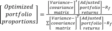
In order to calculate optimized benchmark proportions, the following formula was implemented:
∑
(15)
All stages of the BL method were implemented onto spreadsheet by using VBA programming language.
III. RESULTS
This research considered the problem of managing €10 million portfolio of stocks between 1 June 2004 and 4 August 2009. Portfolio optimization methods were subjects to various constraints, which accounted for different types of risks. The most important is non-negativity. This restriction was introduced for different reasons, but the most important is qualitative – portfolio managers are usually not allowed to take significant short positions, especially when managing portfolios for non-institutional clients.
Results of all optimization approaches will be presented in this section. Performance will be measured on three different factors:
-- Return on Investment (ROI), -- Value at Risk (VaR), -- Sharpe Ratio.
Before evaluating different strategies, methodology for calculating those measures will first be explained.
Return on Investment (ROI)
ROI 16
Where:
V - Initial value of the portfolio ‘y’
V ‐ Final value of the portfolio ‘y’
Value at Risk (VaR)
Daily VaR was monitored on a monthly basis and was calculated by parametric approach, as proposed by Dowd (2008):
17
Where:
- mean investment value of portfolio ‘y’ – volatility of a portfolio ‘y’
- standard normal variable – confidence level
It has to be emphasized that by using parametric approach for calculating VaR, normality of returns was assumed. Inputs for the estimation of VaR were: 30‐days geometric return for each share, variance‐covariance matrix and initial investment at the beginning of each month . Volatility was calculated with the same principle as presented in the equation above. Confidence level for VaR was chosen to be 99%.
Sharpe ratio
In this research Sharpe ratio was calculated by dividing the return on a strategy by the standard deviation of return, as proposed by Damodaran (2003):
Sharpe ratio 18
Where:
– return on portfolio
σ – standard deviation of the portfolio
Sharpe ratio was calculated each month and the final result represents the average of monthly ratios. Monthly Sharpe ratio was calculated each month by taking the average return of an optimization method and dividing it by the standard deviation from the same strategy that month. Standard deviation was calculated in the same manner as already presented in this section of the research.
Interpretation of results
This part represents performance measures of all five portfolio optimization approaches. Results are summarized in the Table IV.
Each financial crisis raises the question whether one can devise a strategy to obtain returns above the market whilst protecting the capital invested. Especially the most recent
developments have emphasized the importance of reliable risk management. It is therefore crucial to study the performance of risk factors, calculated from the optimization outputs.
TABLEIV SUMMARY OF RESULTS
Performance Measure MV Passive EQW BL
ROI -9.28% 14.15% 22.22% 47.31%
VaR99 as % of portfolio
value 2.39% 2.53% 2.59% 2.61%
Sharpe Ratio 0.0335 0.0388 0.0400 0.0431
According to the Table IV, minimum-variance approach represents the safest optimization strategy. Standard deviation of the MV approach is considerable lower than the others. The MV approach aims to optimise portfolio weights so that the optimal solution will be the portfolio with the lowest variance. The empirical results follow that fact.
On the other hand, we developed a method that includes additional factor in the optimization – analysts’ opinions. It is expected that the volatility of the opinions will increase the volatility of the whole portfolio. Higher ‘gross’ risk is therefore expected.
Table IV shows that the TRP strategy significantly outperformed the benchmark in relation to the Sharpe ratio and ROI. Although minimum variance was identified as the safest method, it achieved the lowest return per unit of risk between all five strategies. Benchmark passive investment and the EQW portfolio produced similar results.
We conclude that although incorporating analysts’ opinions increases the riskiness of our portfolio, it yields
significantly higher return per amount of that risk. Investor
who trades off between the risk and return should therefore
choose TRP based strategy, as it will give him the highest
reward for risk they take.
Please note that this article assumed several important factors, which might have changed the outcome. Some of them have directly influenced the performance measures: no transaction costs, no liquidity constraints on selected shares, no taxes, it is possible to trade fractions of shares, no short sales and the sum of the proportions of shares included in the portfolio is always 100% (no cash positions). Investigating performance measures by removing some of the assumptions listed above will be part of the further research.
IV. CONCLUSION
Equity analysts have become an influential factor on the capital markets. Some of the previous researches, such as Womack (1996), Barber et al. (2001) and Espahbodi et al. (2001) even proved that analysts’ coverage is associated with the positive abnormal returns on the stock. These studies focused on the ‘buy’ ratings, issued by analysts.
[image:5.595.300.554.129.195.2]In fact, we obtained results that are not consistent with the efficient market hypothesis (EMH). There are a few possible interpretations for the results; one could say that the investment period is too short and that results were obtained in the ‘non-normal’ market conditions. Others might suggest that assumptions are not realistic. The fact is that our portfolio outperformed the best-performing benchmark by more than 25% and returned 47% ROI in the challenging market conditions. This suggests that there might be time in the future where portfolio managers and traders start considering TRP ratio as one of the factors when they place their buy/sell orders.
In 1991, Schipper showed that the information analysts produce improves the market efficiency by helping investors “to value companies’ assets more accurately”. In line with this statement, we presume that if everyone started using TRP ratio as the proper measure of stock’s value, assets would be priced more efficiently and the opportunity of earning higher abnormal returns would disappear. We therefore conclude that there are clear indications the market currently operates inefficiently, but with more frequent use of this important information, it could become efficient.
ACKNOWLEDGMENT
It is our great pleasure to recognize all those who have helped us with the research. It was a journey through exploring and developing ideas that might help to understand the real value of analysts’ opinions. The authors would like to thank Raiffeisen Bank Maribor, Slovenia, for providing the data used in the research. G. Munda would like to express special gratitude to his mentor, Prof. Peter Oliver of The University of Nottingham, for many helpful thoughts, constructive debate and the feedback on our modest contribution to financial world.
REFERENCES
[1] B. Barber, R. Lehavy, M. McNichols and B. Trueman, “Can investors profit from the prophets? Consensus analyst recommendations and stock returns,” Journal of Finance, vol. ED-56, pp. 341-372,2001. [2] A. Damodaran, Investment Philosophies: Successful strategies and
investors who made them work. New Jersey: Wiley Finance, 2003.
[3] K. Dowd, Measuring market risk. Chichester: John Wiley & Sons, 2008.
[4] R. Espahbodi, A. Dugar, and H. Tehranian, “Further Evidence on Optimism and Underreaction in Analysts’ Forecasts,” Review of
Financial Economics, vol. ED-10, pp. 1-21, 2001.
[5] D. Gujarati, Basic econometrics. New Jersey: McGraw Hill, 2003. [6] P. Kennedy, A guide to econometrics. 5th ed. Bodmin: MPG Books,
2003.
[7] G.S. Maddala, and I.M. Kim, Unit roots, cointegration, and structural
change. Cambridge: Cambridge University Press, 2002.
[8] J.L. Maginn, Managing Investment Portfolios: A Dynamic Process. New Jersey: Wiley Finance, 2007.
[9] H. Markowitz, Portfolio selection: Efficient diversification of
investments. New York: Blackwell Publishing, 1991.
[10] T. Merna, and F.F. Al-Thani, Corporate Risk Management. Chichester: Wiley Finance, 2008.
[11] R. Michaud, “The Markowitz Optimization Enigma: Is Optimized Optimal?” Financial Analysts Journal, vol. ED-45(1), pp. 31-42, 1989.
[12] G. Munda and S. Strasek, “Use of the TRP ratio in selected countries,” Our Economy: review of current problems in economics, vol. ED-57-1, pp. 55-60, 2011.
[13] W.F. Sharpe, G.J. Alexander, and J.V. Bailey, Investments. 6th ed. New York: Prentice Hall, 2006.
[14] A.I. Stonehill and M.H. Moffett, International Financial
Management. Chatham: Taylor & Francis, 1993.