A Beam Search Heuristic for the Multi- commodity Capacitated Multi-facility Weber Problem

A Beam Search Heuristic for the

Multi-commodity Capacitated Multi-facility Weber

Problem

Temel ÖNCAN, M. Hakan AKYÜZ, and İ.Kuban ALTINEL



Abstract—The Multi-Commodity Capacitated Multi-facility Weber Problem (MCMWP) is concerned with locating I capacitated facilities in the plane to satisfy the demand of J customers for K commodities with the minimum total transportation cost. The MCMWP is a non-convex optimization problem. Customer locations, demands and capacities for each commodity are known a priori. The transportation costs, which depend on the commodity type, are proportional to the distance between customers and facilities. We first present a branch and bound algorithm then we propose a beam search heuristic for the MCMWP. According to our computational experiments on randomly generated test instances, we can say that the proposed beam search heuristic

yields comparable results with the previous best heuristics.

Index Terms—Location-allocation, transportation branch

and bound, beam search

I. INTRODUCTION

he Multi-facility Weber Problem (MWP) is an extension of the well-known Weber Problem (WP) which has first been addressed in [1]. The MWP deals with the location of I uncapacitated facilities in the plane to satisfy the demand of J customers at minimum total transportation cost of sending products between facilities and customers. As further extensions of the MWP, we can mention the Capacitated Multi-facility Weber Problem (CMWP) and the Multi-Commodity Multi-facility Weber Problem (MCMWP). Given the locations of J customers and their demands, the CMWP deals with locating I

capacitated facilities in the plane and satisfying the demands of J customers at minimum total transportation cost. The CMWP is shown to be NP-Hard in [2] even when customers are aligned on a straight line. On the other hand, the MCMWP considers the situation where K distinct

commodities are shipped from I capacitated facilities to J

customers with known demands. The transportation costs of both the CMWP and the MCMWP are assumed to be proportional to both the amount shipped and the distance between the facilities and customers. Note that the CMWP reduces to the MWP when the capacity restrictions on facilities are ignored, and the MCMWP reduces to the CMWP when K = 1 holds. In this work we concentrate on the MCMWP which uses ℓr-distance with 1 < r ≤∞.

Manuscript received December 08, 2011. This work was supported in part by TÜBİTAK Grant No: 107M462 and Galatasaray University Scientific Research Projects Grant No: 10.402.001 and 10.402.019. The second author acknowledges the partial support of National Graduate Scholarship Program for PhD Students awarded by TÜBİTAK.

Temel Öncan is with the Department of Industrial Engineering, Galatasaray University, Ortaköy, İstanbul, 34357, TÜRKİYE (phone: +90212-2274480(427); fax: 90212-2595557; e-mail: [email protected]).

M. Hakan AKYÜZ is with the Department of Industrial Engineering, Galatasaray University, Ortaköy, İstanbul, 34357, TÜRKİYE (e-mail: [email protected]).

İ.Kuban ALTINEL is with the Departement of Industrial Engineering, Boğaziçi University, Bebek, İstanbul, 34342, TÜRKİYE (e-mail: [email protected]).

Since its introduction in [3], a considerable amount of research interest has been devoted to the CMWP. As heuristic approaches, we can cite Cooper's [3] early Alternate Location-Allocation (ALA) type heuristic and Aras et al.'s [4] Discrete Approximation (DA) heuristic which is famous for its accuracy. There are also several exact solution approaches. We can mention the complete enumeration procedure in [3] for the Euclidean distance CMWP as an early exact solution algorithm. Then, Sherali and Tunçbilek [5] and Sherali et al. [6] propose branch and bound (BB) algorithms which employ Reformulation Linearization Technique (RLT) (see e.g. [7]) based lower bounding formulations for the squared Euclidean distance CMWP and rectilinear distance CMWP, respectively. The most recent exact solution approach is the BB algorithm developped in [8] for the CMWP which uses ℓr-distance with 1 < r ≤∞. On the other hand, as far as we know, very few studies address the MCMWP. Among them, Akyüz et al. [9] propose a confidence interval approach to estimate lower and upper bounds on the optimal value of the MCMWP. The authors employ several heuristics including an ALA type heuristic, namely the MCALA heuristic, and a randomized DA heuristic. Later on, Akyüz et al. [10] devise approximating MILP formulations and DA heuristics for the MCMWP. These DA heuristics compute both accurate lower and upper bounds on the optimal objective value of the MCMWP by exploiting the properties of the block norms. Recently, a subgradient-like heuristic is suggested in [11] where the authors apply a column generation procedure within a Lagrangean Relaxation (LR) scheme on the MCMWP. Since the MCMWP is more difficult than the CMWP efficient and accurate heuristics are needed for the MCMWP. The motivation of this work is to propose a specially tailored Beam Search (BS) heuristic for the MCMWP. We have tested the proposed BS heuristic on randomly generated test instances and we have observed that the proposed BS heuristic outperforms the best known upper bounding heuristics (i.e. DA heuristics in [10] and [12]) in the literature.

The remainder of this work is organized as follows. In the next section, we present a mathematical programming formulation of the MCMWP. Then in Section 3 we present the location based BB (LBB) algorithm for the MCMWP. Section 4 is where we present the BS heuristic. The computational results and our experiments are reported in Section 5. Finally, we conclude with Section 6.

II.THEMCMWPFORMULATION

Given K commodities, consider a set of J customers for j =

1,…,J, whose known locations are denoted by

with a demand of qjk for each commodity

k and a set of I facilities for i = 1,…, I, whose unknown locations are denoted by with a capacity of

sikfor each commodity k. In addition to the supply quantities

sik and demand quantities qjk, the MCMWP considers also capacity restrictions uijon the amount of total flows between facility i and customer j. Furthermore, let us define decision variables wijk which stand for the unknown amount of commodity k shipped from facility i to customer j having the unit shipment cost of cijk per unit distance which is measured by the ℓr-distance function

1 2

( )

j a aj j

a = T

1 2

( )

i x xi i x = T

( _{i j})

d x a, = 1/ r

r_ 

1 1 2 2

r

i j i j

x a x - a

 _{ }

  with 1 < r ≤∞between facility

i and customer j. Notice that the MCMWP includes two decision variables: the location variables for i = 1,…, I

and the allocation variables wijk for i = 1,…, I; j = 1,…, J;k = 1,…, K. Now we introduce a mathematical formulation of the MCMWP:

i x

min Z =

=1 =1 =1

( , )

I J K

ijk ijk i j i j k

w c d



x a ₍₁₎

s.t.

=1 = J

ijk ik j

w s



i 1, , I ; k 1, , K (2)

=1 = I

ijk jk i

w q



j= 1, , ; = 1, , J k  K

J

J ;

)

(3)

=1 K

ijk ij k

w u



i= 1, , ; = 1, , I j  (4)

0 ijk

w  i= 1,, ; = 1,I j ,

= 1, ,

k  K

(5) This formulation assumes that the MCMWP is balanced, i.e. the total demand and total supply are equal for each commodity. The objective function (1) consists of the sum of total transportation costs. Constraints (2) make sure that the total amount of commodity k produced by facility i

should be exactly shipped. Constraints (3) state that the total amount of commodity k required by customer j should be exactly satisfied. Constraints (4), which are also called as

bundle constraints, enforce that the total amount of allocations on a connection between facility i and customer j

should not be larger than the given upper bound uij. The MCMWP has an optimum solution which always occurs at one of the extreme points of the polyhedron defined by the Multi-commodity Transportation Problem (MTP) polytope which is represented with constraints (2) – (4). Note that

this is guaranteed as long as the transportation costs are expressed as a function of only location variables of the distance . Given such an extreme point and feasible allocations, the MCMWP reduces to pure location problem which further decomposes into I WPs where each of them can be solved by using Weiszfeld's algorithm [13] or its generalizations [14]. The convergence of the Weiszfeld's algorithm for ℓr-norm with 1 < r ≤2is shown in [13]. Therefore, an unconstrained minimization algorithm can be used for the case when r > 2 in order to find the optimal facility locations since the ℓr-norm function is convex.

( _{i j}

d x a,

III. LOCATIONBASEDBRANCHANDBOUNDALGORITHMFOR THEMCMWP

As far as we know, location based BB algorithms date back to the seminal study [15] where the authors suggest the so-called “Big Square Small Square" (BSSS) technique to solve the Obnoxious Facility Problem (OFP). The BSSS technique partitions the plane into smaller squares in which a facility is enforced to be located. The BSSS technique calculates lower and upper bounds for each square. Whenever a lower bound value calculated for a square exceeds the current best known upper bound value, namely the incumbent solution value ZBUB, that square is discarded from further consideration. Otherwise, the BB search process continues with partitioning of this square into four subsquares. Later, Drezner and Suzuki [16] propose to employ triangles instead of squares, namely the “Big Triangle Small Triangle" (BTST). Drezner and Suzuki [16] solve both the OFP and the Weber problem with attraction and repulsion (WAR) by using their BTST technique. A generic approach to solve various single facility location problems by employing the BTST technique is presented in [17]. The underlying idea of both the BSSS and the BTST techniques is to partition the plane into polytopes in which a single facility can be placed. Henceforth, without loss of generality, we employ the terms polytopes and regions interchangeably, in the sequel. To the best of our knowledge, neither the BSSS nor the BTST technique is employed for the MCMWP. Hence, several issues should be carefully handled in order to generalize the BSSS or BTST techniques for the MCMWP. First of all, both of the BSSS and BTST techniques assume that the allocation values are fixed and known a priori which is not the case for the MCMWP. Furthermore, both techniques are designed to use concave lower bounding functions whose minimums occur at one of the extreme points of the regions, namely squares for the BSSS technique and triangles for the BTST technique. Hence, we need novel specially tailored lower bounding methods for the MCMWP. Another critical issue that must be carefully resolved is that during the run of the LBB algorithm some regions can not be directly discarded from consideration for the MCMWP. The LBB algorithm is designed keeping in mind all these issues. We prefer to adopt a BSSS like strategy for the LBB algorithm. We employ a continuous binary partitioning of the location space. For that purpose, we define the following bounds on location variables x_i

1 1

j i j

Initially these bounds are defined as a_in  min_{j ,...,J}₁ {a_in} and a_in  max_{j ,...,J1} { }a_in for both axes n = 1, 2 and i = 1,…, I. This implies that for each facility i the location space is initially selected as the smallest rectangle covering all customers. Observe that, it is also possible to obtain other types of regions than the rectangles defined by (6), by imposing various types of restrictions. These regions can be partitioned by using intersection of different half-spaces. During the run of the LBB algorithm a set of active nodes is kept in the BB tree T. At each step, an active node tT is picked up for exploration according to a predefined

selection criterion. Let denote

facility-region (facility-rectangle) combinations at each node t. Then, a region is selected and partitioned into two complementing subregions (sub-rectangles) and . By complementing subregions, we mean that

holds after the partitioning of , and the interiors of and have no intersecting area (i.e. . This results in two subproblems which further restrict the possible location of facility i. Then, all bounds which restrict the location of the remaining facilities are directly inherited from Ct. A lower and upper bound is calculated for each subproblem, and the ones with a lower bound smaller than the incumbent solution value

ZBUB can be added to the BB tree T. The incumbent solution value ZBUB is updated when a better upper bound is obtained. The LBB algorithm continues until T becomes empty or a stopping condition is satisfied.

1 1

= {( t) ( )}

t I

C x ,R ,..., x , R

t i

R

R

t i

R

2 t i 

t

1 t i I

t i

t I I

2 t i

R

int R

1 2

t t

i i

R R R

t i

R

1

( _it)int R(

1 R

2) = t i

We first describe two specially tailored lower bounding procedures for the MCMWP. They are basically LP based and block norm based approaches. After a brief introduction of each lower bounding procedure, we describe their usage in particular for the LBB algorithm. The lower bounds are used to eliminate unnecessary nodes before adding them to the BB tree T and to check the closeness of the incumbent solution value to optimality. Whenever a region R is partitioned, we face with the subproblems which consist of the constraints (1) – (5) and (6). In order to find lower bounds on these subproblems, we make use of the distance function properties. Given facility-region combinations

, distances are defined as the shortest distance between each facility i assigned to a region

and customer j. Note that,

holds where is the closest point of region to customer j. Lower bounding distances are previously proposed in [18]. For example, when the rectangles are considered the closest point a can be situated on the

rectangle in three different ways. These three cases are illustrated with Fig. 1. In the first case, =

1 1

= {( t) ( )}

t

C x , R ,..., x , R

t i

R

t ij

a

t i

R

t ij

d

(

d d

d

t ij

a

) ( )

t t

ij  aij,aj d x ai, j t i

R

t ij

t ij

j

a

t i

R

R

t ij

d

)

holds when customer j lies within the rectangle (see Fig. 1a). In the second case, is located on one of the borders of (see Fig. 1b). In the third case (see Fig. 1c), is situated at one of the extreme points of when customer j is beyond the area constructed by drawing vertical and horizontal lines on the extreme points of the rectangle containing it. In the first case equals to 0. In the second case, equals to either vertical or horizontal distance from the selected side of . In the third case, equals to the ℓr-norm between the selected extreme point of and customer j. Given the lower bounding distances , we solve the MTP within the LBB algorithm for the MCMWP. Observe that, the distances are constant and do not depend on the location variables xi and holds for i = 1,…, I; j = 1,…,

J. Clearly, implies that (6) is already satisfied and thus, the solution of the MTP provides a lower bound on the LBB subproblems which are represented by constraints (1) – (5) and (6). For the sake of clearness, the LP based lower bound for the MCMWP is explicitly stated as follows:

t i

R

t ij

a

t i t

ij

a

t i

R

t ij

d

t i

R d

d

t ij

d

( t ij i

d d x a

t t ijRi

a

t ij

t ij

j

,

t i

[image:3.595.48.290.84.180.2]

R

Fig. 1. Three possible cases for the closest point a of a

rectangle .

t ij t

i

R

min ZLPt =

=1 =1 =1

: (2) (5) I J K

t ijk ijk ij i j k

w c d

 

 

 

 







(7)

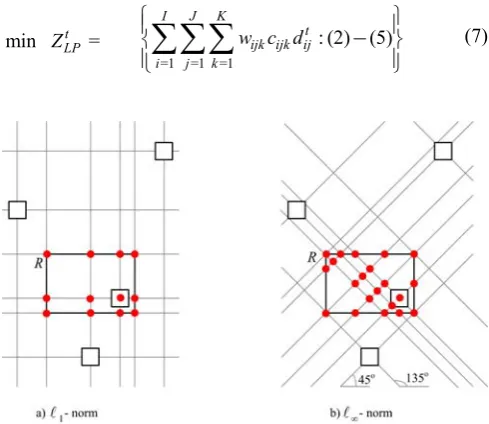
[image:3.595.304.549.517.729.2]

Now we introduce the implementation of the block norm based lower bounding scheme within the LBB algorithm for

the MCMWP. Given a facility- region combination Ct, when the block norms are used, candidate facility locations can be selected from a finite set of intersection points. That is to say, whenever a facility is enforced to lie within a rectangle, the set of candidate facility locations are restricted to lie on that rectangle. When there are no region restrictions on facilities, the optimal facility locations are at the intersection points of the lines drawn on customer locations within their convex hull along the extreme directions of the corresponding block norm. When, we restrict the facilities to be located within the rectangles, the extreme points of the rectangles also play a critical role in the determination of the intersection points. In this case, using the results in [19], the candidate locations consist of the intersection points of the fundamental rays drawn on both the customer locations and the extreme points of regions for i = 1,…, I which are placed either on their borders or within the border. Fig. 2a and Fig. 2b illustrate the intersection points to be considered when ℓr-norm and ℓ1-norm are used, respectively. The rectangle restricting a facility location is denoted by R. Customers are indicated with squares and the intersection points are represented with filled circles. The fundamental rays are drawn on both customer locations and the extreme points of the rectangle R. The resulting candidate points are located either on the intersection of the borders of the rectangle R and a fundamental ray or on the intersection of two fundamental rays. A lower bounding MILP formulation can be proposed to find a block norm based lower bound for the LBB subproblems. Each facility i is restricted to be opened within a region for the LBB subproblems and thus each facility i has its own candidate points within region . On large candidate facility location sets, it is possible to use LR schemes for the LBB subproblems to obtain block norm based lower bounds. For the sake of conciseness, we do not explicitly state these MILPs and LR schemes here. For an interested reader we refer to the studies [10] and [12].

t i

R

t i

R

t i

R

A node of the LBB tree can be prunned without further branching when the lower bound of the current node is larger than the incumbent solution value for the problem. Therefore, it is important to find an accurate upper bound

ZUB, in order to reduce the number of branching operations performed during the run of the LBB algorithm. The initial upper bound value is calculated with the straightforward procedure proposed for the CMWP in [8]. Here, we adapt their approach for the MCMWP by considering all commodity types. The outline of the initial upper bound heuristic as follows.

At the root node, MCALA heuristics are initialized with two different starting allocation sets. The MCALA heuristic solution with the smallest objective value is used as the initial value of ZBUB. For that purpose, the customer locations are enclosed within the tightest rectangle and this rectangle is sliced along the x-axis into I equally spaced intervals. Then, the demand quantities for each commodity in each slice are aggregated and sorted in increasing order. Facilities are also sorted in increasing order of their capacities for all commodities. Lastly, each aggregate demand is assigned to a facility with the same order and the

demands of customers are split among facilities starting from left to right of the x-axis for each commodity. In other words, an unsatisfied demand of customer for a commodity in a slice is merged to the next slice and thus the next facility. Once a feasible transportation plan is obtained, the MCALA heuristic is run. This process is also performed for the y-axis. The best one of these two feasible solutions is considered as the initial upper bound value for the LBB algorithm. Other initial upper bounding procedures can also be implemented for the LBB algorithm. However, we have confined ourselves to use this procedure because of its effciency. Once a lower bound is found for an LBB subproblem, a feasible allocation vector is at hand for the MCMWP at the intermediate LBB nodes. We have also applied a MCALA heuristic and updated the incumbent objective value ZBUB throughout the run of the LBB algorithm when ZUB < ZBUB holds.

The location space associated with an active node of the LBB tree is divided into two subregions. Each of these subregions yields subproblems of the form (1) – (5) and (6). At each partitioning step a rectangle (region) corresponding to facility i is selected and divided into two complementing rectangles (regions) separated by a line. All other facility-region combinations are inherited for new subproblems. A rectangle (region) can be partitioned either vertically or horizontally. For each subproblem, we prefer to partition a rectangle on its longest sides. This implies that if the horizontal (vertical) sides are longer than the vertical (horizontal) sides then, the rectangle is partitioned by connecting the midpoints of two horizontal (vertical) sides. Hence, this helps us to avoid the width (length) of the rectangles to be too large (small) on their vertical (horizontal) sides. As a result, the rectangles are uniformly partitioned on both of their vertical and horizontal sides. The LBB algorithm performs a Best First Search (BFS) strategy. We select an active node tT with the smallest lower bound value for partitioning. At every active node, we keep track of all facility-rectangle (facility-region) combinations (i.e. Ctand for i = 1,…, I) where for each of which lower and upper bound values are calculated. Furthermore, for each rectangle (region) we keep record of its defining extreme points, its area and its parent rectangle. The branching at each node is performed by considering all its rectangles in order to obtain a balanced partitioning. That is to say, we partition the rectangles such that none of the rectangles of the active node t, which is under consideration, has an area greater than twice of the area of the smallest rectangle. Given t and its associated facility-rectangle (facility-region) combination Ct, the branching rectangle is selected with the following strategy.

t i

R

t i

R

t i

R

i*= arg max

i = 1,…, I{ Area of RitCt} (13) Notice that, the branching strategy (13) ensures a balanced partitioning of rectangles. Unless the branching strategy (13) is applied, it is possible to divide a rectangle and its sub-rectangles of the same facility many times which may result in a series of non-improving steps within the LBB algorithm.

possible to partition the location space infinitely many times and this process will not end without applying a suitable stopping condition. Therefore, we can say that a stopping condition plays a crucial role on the termination of the LBB algorithm in acceptable number of iterations. For that purpose, we impose the condition ZLB≥(1- ε) ZBUB to prune the nodes. We set ε = 0.001 in order to avoid excessive computational effort.

IV. ABEAMSEARCHHEURISTICBASEDONTHELBB ALGORITHM

BS is a BB based heuristic search method which dates back to the early study [20] on the speech recognition. BS heuristic performs a breadth-first search (BrFS) strategy on a truncated BB tree. In a complete BB tree search, branching is done such that all possible subproblems are produced and evaluated. This requires a bounding step to calculate lower and upper bounds for each resulting subproblem. On the other hand, BS heuristic considers only the most promising W nodes and performs branching on them. Here W is called as the beam-width and the set of most promising W nodes is named as the beam. In other words, the beam consists of the active nodes which will be considered for further branching in BS heuristic. An active node, which is one of the W nodes in the beam, is further partitioned such that all possible subproblems are generated and the most promising subproblem replaces this active node before the branching. This procedure is repeated for each of the W active nodes which are in the beam. Hence, BS heuristic applies a BrFS strategy in parallel for all W

active nodes in the beam. However, the number of subproblems may become excessive to perform a bounding procedure for each of them when the branching width is quite large, namely there are too many subproblems after a branching step.

In the suggested BS heuristic again only W nodes are allowed to be active in the BB tree. Hence, after each branching operation some of the nodes are discarded from consideration. Promising nodes of the BB tree are considered for further branching according to an evaluation function which is a cost based function. For each active node t, a value Ztis computed using the formula Zt = (1-

)Z_LBt + Z_UBt for 0 ≤≤ 1 where lower and upper bound values t

LB

Z and t UB

Z are associated with Zt. This evaluation function is originally devised in [21]. The BS heuristic performance is significantly affected by the evaluation function used. In our BS heuristic implementation we apply BFS strategy. That is to say, at each branching operation, the most promising active node is selected according to the evaluation function value Zt where tT such that |T| = W. Recall that when BrFS strategy is applied, all of W active nodes at the same level of the BB tree are considered for further branching. However, when BFS strategy is applied within the BS heuristic, only the most promising active node

t with the smallest Zt value is considered for branching. After this single branching step, the most promising W

nodes of the beam, namely the ones having W least Zt values, are kept for further exploration. Moreover, it is also possible to pursue a BrFS strategy in our BS heuristic and branch over W nodes in the beam. However, when BrFS

strategy is employed within our BS heuristic, we have observed that it does not yield better outcomes than the case when the BFS strategy is used. In fact, both BFS and BrFS strategies are equivalent when W = 1. Furthermore, the BFS strategy has helped us to avoid from expensive lower and upper bounding procedures. Note that, in the BS heuristic we employed both LP based and block norm based lower bounding procedures and took into consideration only the one with the largest lower bound value. Lastly, in our BS heuristic for the MCMWP, we have carefully implemented three stopping conditions. The first one is four hour CPU time limit which seems reasonable for most of the instances. As the second stopping condition, whenever the lower bounds of all active nodes are 0.1% or closer to the incumbent solution value, then the BB tree exploration process is terminated. As the third stopping condition, the total number of the rectangles constructed is limited to be 100,000.

V.COMPUTATIONALEXPERIMENTS

All our experiments are performed on a Dell Server PE2900 with two 3.16 GHz. All algoritms are coded in C++

language. Cplex 11.0 with default options is used as a subroutine to solve the resulting LPs and MILPs which are part of the suggested procedures implemented. The MCMWP test set includes two classes of randomly generated instances [12]. The first class consists of 27 instances and the second class consists of 18 instances. The instances in the first class can be considered as “medium” instances and the ones in the second class can be named as “large” instances. As a rule of thumb, medium and large instances satisfy the formula 200 ≤ IJK ≤2000 and 2000 <

CPU times are also reported right after the percent deviation columns corresponding to each heuristic in seconds.

As a general observation, we can assert that the BS heuristic yields better performance for large instances. Observe that, there is a trade-off between the performance of the BS heuristic and the beam-width W. Clearly, the larger the beam-width is, the higher the accuracy and running times are. In general, BS heuristic with beam width W = 3 yields more accurate solutions than the BS heuristic with the beam width W = 1 does.

Medium Instances Large Instances Heuristic

Method

Dev. (%)

CPU (sec.)

Dev. (%)

CPU (sec.)

CL-DA 0.00 83.13 2.83 15680.54 CL-LRDA 10.67 13.20 23.12 1338.18 BS (0,1) 2.70 552.02 7.60 10419.35

BS (0,3) 1.16 1356.46 8.44 12926.41 BS (0.25,1) 1.55 688.03 8.36 10304.36 BS (0.25,3) 0.67 1445.09 8.89 12344.93 BS (0.5,1) 2.91 571.71 10.84 10828.77 BS (0.5,3) 1.59 1477.38 6.99 12027.75

According to our computational experiments we observe the following findings on medium instances. The BS heuristic finds very close solutions (less than 1%) to the best performing heuristic CL-DA. However, CL-DA heuristic yields more efficient results than the BS heuristic does on the average. The BS heuristic is 8% more accurate than the best performing LR heuristic, i.e. CL-LRDA, on the average at the expense of increased CPU times. On large instances, BS heuristic yields 6.99% percent deviations from the best known values in the average. This ratio is 23.12% for the CL-LRDA heuristic which is more efficient than the BS heuristic. However, the best performing heuristic CL-DA could not produce solutions in 7 out of 18 test instances within four hour of time limit on large instances. In 6 out of these 7 test instances for which the CL-DA could not even found solutions, the BS heuristic outperforms the CL-LRDA heuristic in terms of accuracy. On the average, the BS heuristic with the worst performing (,W) setting, namely with the setting (0, 3) has percent deviation of 9.79% while the CL-LRDA heuristic yields percent deviation of 23.26% on the average of these 7 instances. In short, BS heuristic produces highly competitive results with the DA heuristics which are famous for their accuracy.

VI. CONCLUSION

BS heuristics are popular algorithms which are based on BB procedures. The BS heuristic searches over a truncated BB tree using a BrFS strategy and branches only on its most promising W nodes. To the best of our knowledge, this is a pioneering work which suggests a BS heuristics on the MCMWP. Moreover, the proposed BS heuristic yields promising performance. According to our extensive computational experiments on randomly generated test instances, we have observed that the proposed BS heuristics yield comparable results with the best heuristics from the

literature. In more than half of the test instances, the BS heuristic yields the best solutions.

REFERENCES

[1] L. Cooper, “Location-allocation problems”, Oper. Res., vol. 11, no. 3, pp. 331–343.

[2] H. D. Sherali and F.L. Nordai, “NP-hard, capacitated, balanced p-median problems on a chain graph with a continuum of link demands”, Math. Oper. Res., vol. 13, no. 1, pp. 32–49, 1988.

[3] L. Cooper, “The transportation-location problem”, Oper. Res., vol. 20, no. 1, pp. 94–108, 1972.

[4] N. Aras, İ. K. Altınel and M. Orbay, “New heuristic methods for the capacitated multi-facility Weber problem”, Nav. Res. Log., vol. 54, no. 1, pp. 21–32, 2007.

TABLEI

THE AVERAGE PERFORMANCE OF THE CL-DA,CL-LRDA AND BS

HEURISTICS VS.DA HEURISTIC

[5] H. D. Sherali and C. H. Tunçbilek, “A Squared-Euclidean distance location-allocation problem”, Nav. Res. Log., vol. 39, no. 4, pp. 447– 469, 1992.

[6] H. D. Sherali, S. Ramachandran, and S. I. Kim, “A localization and reformulation discrete programming approach for the rectilinear distance location-allocation problems”, Discrete Appl. Math., vol. 49, no. 1-3, pp. 357–378, 1994.

[7] H. D. Sherali and W. P. Adams, A reformulation-linearization

technique for solving discrete and continuous nonconvex problems.,

Dordrecht, The Netherlands: Kluwer Academic Publishers, 1999. [8] H. D. Sherali, I. Al-Loughani, and S. Subramanian, “Global

optimization procedures for the capacitated Euclidean and ℓpdistance

multifacility location-allocation problem”, Oper. Res., vol. 50, no. 3, pp. 433–448, 2002.

[9] M. H. Akyüz, T. Öncan, and İ. K. Altınel, “The multi-commodity capacitated multi-facility Weber problem: heuristics and confidence intervals”, IIE Trans., vol. 42, no. 12, pp. 825–841,2010.

[10] M. H. Akyüz, T. Öncan, and İ. K. Altınel, “Efficient approximate solution methods for the multi-commodity capacitated multi-facility Weber problem”, Comput. Oper. Res., vol. 39, no. 2, pp. 225–237, 2012.

[11] M. H. Akyüz, T. Öncan, and İ. K. Altınel, “Solving the multi-commodity capacitated multi-facility Weber problem using Lagrangean relaxation and a subgradient-like algorithm”, J. Oper.

Res. Soc., to be published with doi:10.1057/jors.2011.81.

[12] M. H. Akyüz, “Location Allocation Problems with Multi-commodity Flows: Exact and Aproximate Solution Methods”, Ph.D. Dissertation, Dept. Ind. Eng., Boğaziçi Univ., İstanbul, Türkiye, 2011.

[13] E. Weiszfeld, “Sur le point lequel la somme des distances de n points donnés est minimum”, Tôhoku Math. J., vol. 43, no. 1, pp. 355–386, 1937.

[14] J. Brimberg, and R. F. Love, “Global convergence of a generalized iterative procedure for the minisum location problem with ℓp

distances”, Oper. Res., vol. 41, no.6, pp. 1153–1163, 1993.

[15] P. Hansen, P. D. Peeters, and J. F. Thisse, “On the location of an obnoxious facility”, Sistemi Urbani, vol. 3, pp. 299–317, 1981. [16] Z. Drezner and A. Suzuki, “The big triangle small triangle method for

the solution of nonconvex facility location problems”, Oper. Res., vol. 52, no. 1, pp. 128–135, 2004.

[17] Z. Drezner, G. O. Wesolowsky, and T. Drezner, “A general global optimization approach for solving location problems in the plane”. J.

Global Optim., vol. 37, no. 2, pp. 305–319, 2007.

[18] P. Hansen, P. D. Peeters, D. Richard, and J. F. Thisse, “The minisum and minimax location problems revisited”, Oper. Res., vol. 33, no. 6, pp. 1251–1265, 1985.

[19] J. F. Thisse, J. E. Ward, and R. E. Wendell, “Some properties of location problems with block and round norms”, Oper. Res., vol. 32, no. 6, pp. 1309–1327, 1984.

[20] B. T. Lowerre, “The HARPY speech recognition system”, Ph.D. Dissertation, Dept. Comput. Sci., Carnegie-Mellon Univ., Pittsburgh, PA, 1976.