DT_sv1_min_obs_servo_driver.m and a corresponding Simulink file DT_sv1_min_obs_servo.mdl. Modify this new file to implement state variable feedback using

ECE-520: Discrete-Time Control Systems Homework 8

Due: Tuesday February 6

In this homework we will simulate and study minimum order observers coupled with state variable feedback, and then we will add on integral control.

Minimum order observers only estimate those states we don’t know or can’t measure. If a state is know, the minimum order observer uses that state.

For the first four problems, utilize the continuous time torsional system models available from the class website.

1a) Copy your program DT_sv1_observer_driver.m to DT_sv1_min_obs_driver.m You will need to modify the part of the code that determines the observer gains, and you will have to have the program call the simulation DT_sv1_min_observer.mdl. Copy the Simulink file DT_sv1_observer.mdl to DT_sv1_min_observer.mdl . Modify this new file to implement state variable feedback using a minimum order observer to estimate the states for a one degree of freedom system. In addition, you will need to modify your code so that you can utilize different sampling rates.

Assume we want the state vector written as

[

]

H

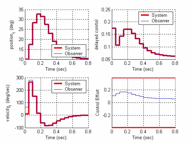
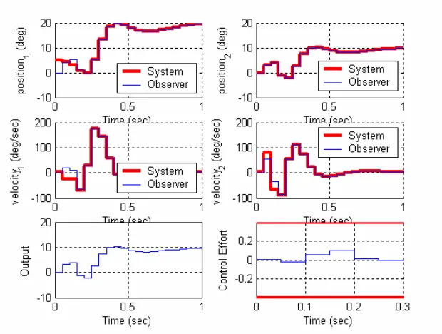
b) Assume the only known state is the position, and the output is the position of the disk. Use a sampling interval of 0.05 seconds, assume all the state feedback poles are at 0.5, and the observer poles are at 0.2 and 0.3. Also assume the system initially starts at a position of 10 degrees, with an initial velocity of 10 degrees, and an initial delayed input of 10 degrees (be careful of units here! The model works in radians.). The initial estimates of the observer are zero. For a 10 degree step input you should get the graph shown in Figure 1. Turn in your plot.

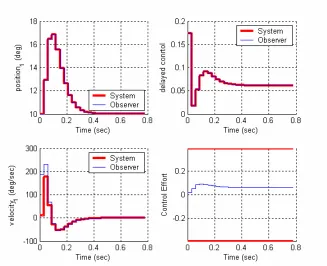
c) Now assume the same initial conditions as in part a, but both the position of the disk and the delayed input signal are known. The observer pole is placed at 0.3 and the sampling interval is still at 0.05. For a 10 degree step input you should get the graph shown in Figure 2. Turn in your plot.

Figure 1. Results for problem 1b.

Figure 3. Results for problem 1d.

2) Now we want to combine the minimum observer and state feedback with integral control for the one degree of freedom system.

a) Create a driver file DT_sv1_min_obs_servo_driver.m and a corresponding Simulink file DT_sv1_min_obs_servo.mdl. Modify this new file to implement state variable feedback using a minimum order observer to estimate the states for a one degree of freedom system. In

addition, you will need to modify your code so that you can utilize different sampling rates. Assume we want the state vector written as

[

]

to reflect this new ordering. You also need to fix the demuxes in your Simulink file to reflect this new order.

H

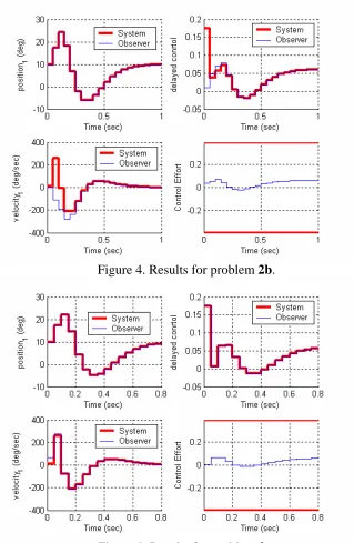
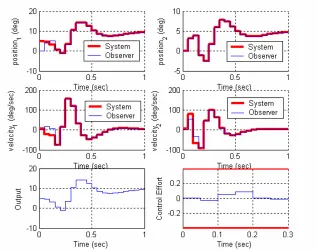
b) Assume the only known state is the position, and the output is the position of the disk. Use a sampling interval of 0.05 seconds, assume all the state feedback poles are at 0.5, and the observer poles are at 0.2 and 0.3. Also assume the system initially starts at a position of 10 degrees, with an initial velocity of 10 degrees, and an initial delayed input of 10 degrees (be careful of units here! The model works in radians.). The initial estimates of the observer are zero. For a 10 degree step input you should get the graph shown in Figure 4. Turn in your plot.

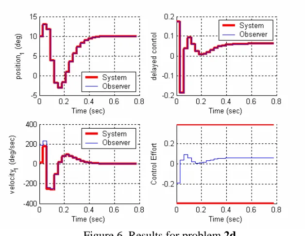
d) Now assume the same conditions as part c, but with a sampling interval of 0.03 seconds, For a 10 degree step input you should get the graph shown in Figure 6. Turn in your plot.

Figure 4. Results for problem 2b.

Figure 6. Results for problem 2d.

3) Copy your program DT_sv2_observer_driver.m to DT_sv2_min_obs_driver.m You will need to modify the part of the code that determines the observer gains, and you will have to have the program call the simulation DT_sv2_min_observer.mdl. Copy the Simulink file DT_sv2_observer.mdl to DT_sv2_min_observer.mdl . Modify this new file to implement state variable feedback using a minimum order observer to estimate the states for a one degree of freedom system. In addition, you will need to modify your code so that you can utilize different sampling rates.

Assume we want the state vector written as

[

]

G H

You also need to modify the get_desired_states variable as follows so the ECP system will put your states in this order:

get_desired_states = [0 0 1 0 0 0 0 0; 1 0 0 0 0 0 0 0; 0 1 0 0 0 0 0 0; 0 0 0 1 0 0 0 0];

b) Assume the only known state is the position of the second disk, and the output is the

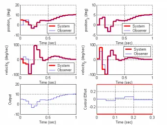
c) Same conditions as in b, but assume the output is the second disk. For a 10 degree step input you should get the graph shown in Figure 8. Turn in your plot.

d) Same conditions as b, but now the positions of both disk 1 and disk 2 are known (the output is the position of the first disk). Place the state feedback poles all at 0.2 and the observer poles at [0.01 0.015 0.02]. For a 10 degree step input you should get the graph shown in Figure 9. Turn in your plot.

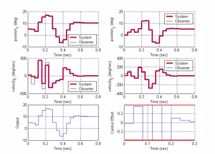
e) Same conditions as d, but the sampling interval is now 0.035. For a 10 degree step input you should get the graph shown in Figure 10. Turn in your plot

Figure 8. Results for problem 3c.

Figure 10. Results for problem 3e.

4) Now we want to combine the minimum observer and state feedback with integral control for the two degree of freedom system. Create a driver file DT_sv2_min_obs_servo_driver.m and a corresponding Simulink file DT_sv2_min_obs_servo.mdl. Modify this new file to

implement state variable feedback using a minimum order observer to estimate the states for a two degree of freedom system. In addition, you will need to modify your code so that you can utilize different sampling rates.

Assume we want the state vector written as

[

]

T d

x x x x u . You need to modify both

and to reflect this new ordering. You also need to fix the demuxes in your Simulink file to reflect this new order.

G H

You also need to modify the get_desired_states variable as follows so the ECP system will put your states in this order:

get_desired_states = [0 0 1 0 0 0 0 0; 1 0 0 0 0 0 0 0; 0 1 0 0 0 0 0 0; 0 0 0 1 0 0 0 0];

b) Assume the only known state is the position of the second disk, and the output is the

delayed input is assumed to be 0. The initial estimates of the observer are zero. For a 10 degree step input you should get the graph shown in Figure 11. Turn in your plot.

c) Same conditions as in b, but assume the output is the second disk. For a 10 degree step input you should get the graph shown in Figure 12. Turn in your plot.

d) Same conditions as b, but now the positions of both disk 1 and disk 2 are known (the output is the position of the first disk). Place the state feedback poles all at 0.2 and the observer poles at [0.01 0.015 0.02 ]. For a 10 degree step input you should get the graph shown in Figure 9. Turn in your plot.

e) Same conditions as d, but the sampling interval is now 0.04. For a 10 degree step input you should get the graph shown in Figure 10. Turn in your plot

Figure 12. Results for problem 4c.

Preparation for Lab

5) You should load your continuous time models (from labs 1 and 2) into your Matlab driver files so you will be able to try sampling at different rates. You only need to simulate the torsional systems (or only the rectilinear systems). You can change the sampling interval if it helps you get better responses, but don’t use a sampling interval smaller than 0.02 seconds. Assume both your system and the observer states are all zero at the beginning of the

simulation. (You will most likely not be able to see any difference between the estimated and true states.) Your system should meet the following contstraints:

For a 10 degree step input:

• the settling time for your system is less than 1 s

• the percent overshoot for your system is less than 20% • the control effort does not hit a limiter (does not saturate) • the steady state error is zero

a) For your one degree of freedom model, utilizing state variable feedback and a minimum order observer (no integral control). Assume the position of the disk is available to the observer.

b) For your one degree of freedom model, utilizing state variable feedback, a minimum order observer, and integral control. Assume the position of the disk is available to the observer.

c) For your two degree of freedom model, utilizing state variable feedback and a minimum order observer (no integral control). Assume the positions of both disks are available to the observer, and you want to control the position of the first disk.

d) For your two degree of freedom model, utilizing state variable feedback, a minimum order observer, and integral control. Assume the positions of both disks are available to the observer, and you want to control the position of the second disk.