An algebraic multigrid method for high order time discretizations of the div grad and the curl curl equations

An algebraic multigrid method

for high order time-discretization of

the div-grad and the curl-curl equations

Tim Boonen

Jan Van lent

Stefan Vandewalle

Report TW 483, December 2006

Katholieke Universiteit Leuven

Department of Computer Science

An algebraic multigrid method

for high order time-discretization of

the div-grad and the curl-curl equations

Tim Boonen

Jan Van lent

Stefan Vandewalle

Report TW 483, December 2006

Department of Computer Science, K.U.Leuven

Abstract

We present an algebraic multigrid algorithm for fully coupled implicit Runge-Kutta and Boundary Value Method time discretiza-tions of the div-grad and curl-curl equadiscretiza-tions. The algorithm uses a blocksmoother and a multigrid hierarchy derived from the hierarchy built by any algebraic multigrid algorithm for the stationary version of the problem. By a theoretical analysis and numerical experiments, we show that the convergence is similar to or better than the con-vergence of the scalar algebraic multigrid algorithm on which it is based. The algorithm benefits from several possibilities for imple-mentation optimization. This results in a computational complexity which, for a modest number of stages, scales almost linearly as a function of the number of variables.

Keywords :div-grad equation, curl-curl equation, implicit Runge-Kutta meth-ods, boundary value methmeth-ods, algebraic multigrid

An algebraic multigrid method

for high order time-discretization of

the div-grad and the curl-curl equations

Tim Boonen

,

Jan Van lent

,

Stefan Vandewalle

Abstract

We present an algebraic multigrid algorithm for fully coupled implicit Runge-Kutta and Boundary Value Method time discretizations of the div-grad and curl-curl equations. The algorithm uses a blocksmoother and a multigrid hierarchy derived from the hierarchy built by any algebraic multigrid algorithm for the sta-tionary version of the problem. By a theoretical analysis and numerical experi-ments, we show that the convergence is similar to or better than the convergence of the scalar algebraic multigrid algorithm on which it is based. The algorithm benefits from several possibilities for implementation optimization. This results in a computational complexity which, for a modest number of stages, scales almost linearly as a function of the number of variables.

1

Introduction

Implicit Runge-Kutta (IRK) and Boundary Value Method (BVM) time discretizations have many appealing properties, such as high order of accuracy and good stability [7, 9, 10, 6]. However, when applied to time-dependent partial differential equations, they give rise to linear systems which are difficult to solve. First of all, the size of these systems is a multiple of the size of the systems to be solved for the backward Euler (BE) discretization of the same problem. Also, the efficiency of existing direct and iterative solvers for BE discretizations usually significantly deteriorates when applied to IRK or BVM discretizations.

In the case of IRK methods, the computational cost can be reduced significantly by using diagonally implicit (DIRK) Runge-Kutta methods. The resulting system is then block-triangular, and can be solved as a sequence of smaller problems. These smaller problems have a similar structure as the one to be solved in the BE method, hence efficient solvers for that method can be reused. Unfortunately, DIRK methods have a lower order of accuracy and poorer stability properties than fully coupled IRK methods of the same size [7, 10]. This order and stability reduction can be avoided by using a DIRK method as a preconditioner for the fully coupled IRK system [15]. The algorithm developed in [15] allows the reuse of existing BE software components.

∗_{Department of Computer Science, Katholieke Universiteit Leuven,small Celestijnenlaan 200A, B-3001} Leuven, Belgium; email: {Tim.Boonen,Stefan.Vandewalle}@cs.kuleuven.be. Tim Boonen is research as-sistant of the Fund for Scientific Research - Flanders (Belgium) (F.W.O.-Vlaanderen).

Unfortunately, the number of iterations required for solving the preconditioned IRK-system increases rapidly with the number of stages in the IRK method.

In [20], it is shown how geometric multigrid techniques can be used to solve ef-ficiently fully coupled IRK and BVM time discretizations of finite difference spatial discretizations of time-dependent parabolic problems

−∇·(α·∇V) +β∂V

∂t =ρ, α>0,β≥0. (1)

The key is the use of a blocksmoother updating all unknowns related to a grid point simultaneously. In this paper, the approach of [20] will be extended to algebraic multi-grid (AMG) for (1) and for the curl-curl equation

~_∇×(α~_∇×~_{A) +β}∂~_A

∂t =~J, α>0,β≥0. (2)

Equation (2) arises in time-domain approaches for solving electromagnetic problems, such as the eddy current problem [16, 4].

A theoretical estimate of the complexity of the AMG algorithm developed in this paper would lead one to conclude that the number of floating point operations and the memory requirements scale cubically and quadratically respectively as a function of the number of stages in the IRK or BVM method. It will be shown, however, that the algorithm offers several opportunities for implementation optimization, yielding a significant increase of the floating point execution rate and a significant reduction of the memory requirements. The timing results of the optimized implementation will be shown to scale rather linearly as a function of the number of stages. Thanks to the favorable timings and memory requirements and to the high order of accuracy of the considered time discretization methods, the presented AMG algorithm is very useful in practice.

This paper is organized as follows. In Section 2, the discretizations in time and space of (1) and (2) used in this paper, are explained. In Section 3, the block AMG algorithm is discussed, and in Section 4 a convergence analysis is presented. Section 5 deals with important implementation issues. In Section 6, some numerical results are presented that illustrate the efficiency of the method.

2

Spatial and temporal discretization

For (1), we consider standard lowest order spatial discretizations using finite differ-ences or finite elements conforming in H1(Ω). For (2), we consider spatial discretiza-tions using the finite integration technique (FIT) [8] or using lowest order edge finite elements conforming in H(curl;Ω)[11]. In that case, the degrees of freedom (DoF) are associated with the edges of the mesh. For both problem types, the considered spatial discretizations give rise to the following set of equations:

Ku+Mdu

dt =h. (3)

The system size, denoted as N, equals the number of nodes or edges for the div-grad and the curl-curl problem respectively. The symmetric and positive definite matrices

K∈RN×Nand M∈RN×Ndenote the stiffness matrix and the mass matrix. The vector

h∈RN _{is the vector of excitations.}

and for the case of the curl-curl equation to [13, 1, 2]. In this paper, IRK and BVM time discretization (see [7, 9, 10, 6]) will be used. For the reader’s convenience, and in order to introduce some essential notation, we shall recall some of the basic formulas and properties of these methods.

Consider the system of N ODEs

du

dt =f(t,u), with u(t0) =u0∈R

N_{. (4)}

An implicit Runge-Kutta (IRK) method (see [7, 9, 10]) approximates the solution

u(t0+∆t)by u1, computed from

u1 = u0+∆t

s

∑

j=1

bjf(t0+cj∆t,xj). (5)

Here, s denotes the number of stages. The s vectors xi∈RN satisfy the following

system of equations

xi = u0+∆t

s

∑

j=1

ai jf(t0+cj∆t,xj), i=1. . .s. (6)

With Airk= [ai j]∈RN×N, birk= [b1 ... bs]T ∈RN and fj= f(t0+cj∆t,xj)∈RN,

and using the multivectors X = [x1 ...xs]∈RN×s, U0= [u0 ...u0]∈RN×s and F=

[f1... fs]∈RN×s, (5) and (6) can be rewritten compactly as

u1 = u0+∆tFbirk (7)

X = U0+∆tFATirk. (8)

Boundary value methods (BVM) can be considered a generalization of linear

multi-step methods (LMM) (see [6]). In each multi-step of a BVM, the solution values at a series of n points in time t1,t2, . . . ,tnare approximated. Here, for simplicity of notation, we

shall only consider the equidistant case, where tj=t0+j∆t. A k-step BVM for (4) has for each i=k1, ...,n−k2, with k1+k2=k, an equation of the form

k2

∑

j=−k1

αk1+jui+j=∆t

k2

∑

j=−k1

βk1+jf(ti+j,yi+j). (9)

The main difference with traditional LMM time discretization is the use of future points in time. As such, a BVM discretization cannot be solved in a time-marching way. An additional k1−1 initial and k2final equations are needed of the form

∑k j=0α

(i)

j uj = ∆t∑ki=0β

(i)

j f(tj,uj) i=1, ...,k1−1

∑k j=0α

(i)

j un−k+j = ∆t∑kj=0β

(i)

j f(tn−k+j,un−k+j) i=n−k2+1, ...,n.

(10)

The coefficientsα(_ji)andβ(_ji)are chosen such that the truncation errors are of the same order as for the basic method (9). When applied to (3), the BVM problem reads in compact format:

Here, u0and f0represent the initial condition and the corresponding right-hand side value at time t0. The matrices Abvm,Bbvm∈Rn×nhave a quasi-Toeplitz structure. For

instance,[a0Abvm]is given by

[a0Abvm] =

                  α1

0 α11 . . . α1k

..

. ...

αk1−1

0 α

k1−1

1 . . . α

k1−1

k

α0 . . . αk

. .. . ..

α0 . . . αk

αn−k2+1

0 . . . α

n−k2+1

k

..

. ...

αn

0 . . . αnk

                  (12)

Assuming that Abvmis invertible, (11) can be transformed into a system of the form (8):

U = −u0aT0+∆t f0bT0

A−T_bvm+∆tFBT_bvmA−T_bvm := _U˜_{0+∆tF ˜A}T_{. (13)}

The computational cost for IRK and BVM methods is dominated by the solution of (8) and (13) respectively. Thanks to the formal equivalence of these systems, the ana-lysis in this paper can be restricted to IRK problems and the results will carry over automatically to BVM problems when Airkis replaced by A−bvm1Bbvm/n. Note that the

scaling factor 1/n takes into account the specific meaning of the time step∆t. For IRK

methods, it corresponds to the global time step; for BVM methods, it is the time step

between the intermediate steps.

We will now derive three formulations for the linear system that appears in every time-step when an IRK method is applied to the semi-discretized PDE. The application of (6) to (3) yields a system of the following form, with Isthe unit matrix of size s:



 

M+∆tKa11 . . . ∆tKa1s

..

. ...

∆tKas1 . . . M+∆tKass

      ˜ x1 .. . ˜ xs  

 = ˜b. (14)

With⊗the Kronecker matrix product symbol, (14) can be written in tensor form:

(Is⊗M+∆tAirk⊗K)x˜ = ˜b. (15)

Here, the unknowns are ordered block-wise; the vectors ˜xi∈RNcorrespond to the

un-knowns of the ith IRK stage. If Airkis triangular, as for DIRK methods, (14) can be

solved efficiently with block back-substitution using solvers optimized for BE prob-lems. This is because the diagonal blocks of (14) are formally equivalent to BE dis-cretizations with a scaled time step∆˜t=aii∆t. In fully coupled IRK discretizations,

however, it is not possible any more to solve for the ˜xivalues sequentially.

Reordering the unknowns in (14) per node for div-grad problems and per edge for curl-curl problems yields a system of the following form:



 

m11Is+∆tk11Airk · · · m1NIs+∆tk1NAirk

..

. . .. ...

mN1Is+∆tkN1Airk · · · mNNIs+∆tkNNAirk

      x1 .. . xN  

which is equivalent to

(M⊗Is+∆tK⊗Airk)x = b. (17)

Here, xi∈Rsdenotes the vector of the stage values related to the node respectively edge

i. Formulation (16) will be used to explain the block AMG method presented in this

paper. The third formulation, which will prove useful for implementation purposes, stems from the application of (8) to (3). This yields:

MX+∆tKX AT_irk = B. (18) Note that (15), (17) and (18) are mathematically equivalent. Once these systems have been solved, (5) or (7) can be used to propagate the solution values from t0to t1.

3

Block AMG algorithm

In this section, an algebraic multigrid algorithm is developed for problems of the form (15)-(17)-(18), denoted in short as Lx=b. A standard multigrid cycle is considered,

which is the recursive application of the following 2-level scheme:

1. smoothing on Lx=b

2. restriction: bc=Rirk(b−Lx)

3. (approximate) solve of Lcxc=bc

4. prolongation: x←x+Pirkxc

5. smoothing on Lx=b

Here, the subscript c refers to the coarse level; the matrices Pirkand Rirkare the

prolon-gation and restriction matrices respectively. In order to characterize the algorithm, a procedure to build Pirkand Rirkand the coarse system matrices Kcis needed. Also, the

smoothing operation is to be specified. For the solution of the system at the coarsest level of the multigrid hierarchy, a direct solver or a preconditioned Krylov solver can be used.

3.1

Prolongation and restriction

We suggest to derive the prolongation matrix Pirkfrom the prolongation matrix P built

for the stationary problem Kx=b, where K is the stiffness matrix from (3). The matrix P can be built using any of the classical AMG heuristics, for instance [18, 19, 17, 5]

for the div-grad problem and [13, 1, 2] for the curl-curl problem. More precisely, for formulation (17), the following construction is suggested for Pirk:

Pirk = P⊗Is. (19)

Note that this amounts to stage decoupling for the prolongation operator. Following the standard AMG practice, we set the restriction operator equal to the prolongator’s transpose, that is

Using the compact formulation of (18), the restriction of the residual and the prolonga-tion of the coarse grid correcprolonga-tion read:

Bc = PT B−MX−∆tKX ATirk

(21)

X ← X+PXc (22)

3.2

Construction of the coarse system

As for any AMG method, the coarse system matrices are built as the Galerkin product of the fine system matrices and the prolongation matrices. For the formulation used in (17), we have

Lc = PirkT (M⊗Is+∆tK⊗Airk)Pirk

= PTMP⊗Is+∆t PTKP

⊗Airk. (23)

Using the compact format of (18), the coarse system reads:

PTMPXc+∆t PTKPXcATirk=Bc. (24)

Note that (24) corresponds to the classical IRK time-discretization of the coarse grid equivalent problem to (3), i.e.

Kcu+Mc

du

dt =hc, with Kc=P

T_{KP and M}

c=PTMP.

3.3

Definition of the smoother

For the div-grad equation (1), the blocksmoother suggested in [20] for use with a geo-metric multigrid method, will be used. This smoother consists of a sequence of local solves, one corresponding to each node i, in which all stage values for that node are updated simultaneously:

(miiIs+∆t kiiAirk)xi = bi−

∑

(mi jIs+∆t ki jAirk)xj. (25)

This blocksmoother is a block Gauss-Seidel type matrix splitting iteration applied to (16). Using the matrix splittings M=M++M− and K=K++K−, with M+ and

K+denoting the lower triangular parts of M and K, (25) can be formulated in tensor notation as:

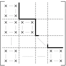
M+⊗Is+∆tK+⊗Airkx[ν+1]=b− M−⊗Is+∆tK−⊗Airkx[ν]. (26)

Here, superscript[ν]is used to denote the iteration index. The nonzero structure of the lefthand side matrix is indicated in Figure 1. Note that the same matrix splittings, applied to a backward Euler discretization of (3), correspond to a classical Gauss-Seidel iteration for the problem(M+∆tK)x=b,

M++∆tK+

x[ν+1] = b− M−+∆tK−

Figure 1: Nonzero structure of M+⊗Is+∆tK+⊗Airk.

[16]). The latter reads, with f denoting the number of mesh faces, and with G∈Re×n

and C∈Rf×e_{respectively the discrete gradient and curl operators}

Re₌ran(G)⊕ran(CT). (28) We refer the reader to [12] for an analysis of this phenomenon. In this paper, the so-called hybrid smoother, presented in [12], will be used. This smoother performs an additional smoothing step in ran(G)on an auxiliary system. The system matrix Laux

of this auxiliary system is usually constructed as the Galerkin product of the original system matrix with the gradient matrix G.

For our purposes, a block version of the hybrid smoother is needed. The auxiliary system matrix is constructed as the Galerkin product of the original system matrix with the decoupled tensor version Girk=G⊗Isof the gradient:

Laux = GTirk(M⊗Is+∆tK⊗Airk)Girk

= GTMG

⊗Is+∆t GTKG⊗Airk. (29)

Using the compact format of (18), the auxiliary system reads:

GTMGXaux+∆t GTKG

XauxATirk=Baux. (30)

Note that GTKG is zero away from the Dirichlet boundaries. One step of the block

hybrid smoother is defined as follows:

1. smoothing on (18)

2. block restriction: Baux=GT(B−MX−∆tKX AT_irk)

3. smoothing on (30)

4. block prolongation: X←X+GXaux

5. smoothing on (18)

Formally, this is equivalent to a 2-level multigrid cycle with prolongator Girkand coarse

4

Convergence analysis

4.1

A formula for the asymptotic convergence factor

The convergence analysis for the AMG method presented in this paper is similar to the convergence analysis for the geometric multigrid method in [20]. First, we analyze the blocksmoother. To this end, we consider the matrix function

S(z) = −(zK++M+)−1(zK−+M−). (31) Note that S(∆t)is the iteration matrix for the Gauss-Seidel iteration defined by (27) for the BE discretization of (3) with a time step ∆t. The iteration matrix for the

blocksmoother (26) for the IRK discretization of the same problem can be written in terms of the matrix function (31) as well. It is given by S(∆Airk), which equals

− ∆tAirk⊗K++ Is⊗M+−1 ∆tAirk⊗K−+ Is⊗M−. (32)

Using the eigenvalue decomposition Airk=VΛV−1 and after applying the Butcher

transformation, which is the similarity transformation corresponding to IN⊗V (see

[7]), (32) can be shown to be equivalent to

− ∆tΛ⊗K++Is⊗M+−

1 _∆

tΛ⊗K−+Is⊗M−.

This shows that (32) is spectrally equivalent to the following block diagonal matrix:

S(∆tAirk)∼



 

S(∆tλ1) · · · 0 ..

. . .. ... 0 · · · S(∆tλs)





, λi∈σ(Airk).

Here,σ(Airk)denotes the spectrum of Airk, which is complex for most fully coupled

IRK and BVM methods. So, the asymptotic convergence behavior of the blocksmoother (26) for the IRK discretization can be analyzed using the convergence results for the corresponding Gauss-Seidel smoother (27) for the BE discretization of the same prob-lem. Withρ(A)denoting the spectral radius of A, the asymptotic convergence factor for the blocksmoother is given by:

ρ(S(∆tAirk)) = max

λ∈σ(Airk)

ρ(S(∆tλ)). (33)

A similar analysis can be done for a two level multigrid cycle using the matrix function

T(z) =S(z)ν2_I

e−P PT(zK+M)P −1

PT(zK+M)S(z)ν1_,

whereν1andν2are the number of pre- and post-smoothing iterations. Here, the invari-ance of the prolongation matrix Pirkfor the similarity transformation IN⊗V is used:

IN⊗V−1·(P⊗Is) (IN⊗V) = (IN·P·IN)⊗ V−1·Is·V=P⊗Is.

The results are analogous to (33), i.e.

ρ(T(∆tAirk)) = max

λ∈σ(Airk)

By recursion, the results for the two level cycle immediately carry over to a multilevel cycle. The analysis for the block hybrid smoother is formally identical to the analysis for the two level cycle, with P replaced by G.

To summarize, the asymptotic convergence of the presented IRK AMG algorithm is related to the asymptotic convergence behavior of the corresponding AMG algorithm applied to the BE discretization of the same problem, but with a scaled time step. That is, the asymptotic multigrid convergence factor for the fully coupled IRK system (16) corresponds to the worst case of the asymptotic multigrid convergence for the problems

(λi∆tK+M)x=b, withλi∈σ(Airk). (35)

The latter can be analyzed quantitatively by a so-called local Fourier mode analysis [18, 21, 14, 3]. Note that (33) and (34) continue to hold for BVM time discretizations if Airkis replaced by A−bvm1Bbvm/n, as mentioned in Section 2.

4.2

Discussion

The convergence speed of multigrid for the BE problem(∆tK+M)x=b depends on

the value of∆t. Hence, in order to be able to interpret (35), knowledge of the location

of the eigenvalues λi is of great importance. The location in the complex plane of

the eigenvalues of Airkand A−_bvm1Bbvm/n for some popular IRK and BVM methods is

indicated in Figure 2. The picture is very similar for the classical IRK families of type RadauIA, RadauIIA, Gauss and LobattoIIIC and for the BVM family GAM. For the IRK families LobattoIIIA and LobattoIIIB, Airkis singular and one eigenvalue is 0. For

the BVM family GBDF with more then 5 intermediate steps, some eigenvalues have a (small) negative real part. Typically, the modulus of the eigenvalues decreases with increasing number of stages for IRK or intermediate steps for BVM, and the decrease becomes smaller with increasing number of stages or steps.

For a model problem on a regular grid, the asymptotic convergence factor of a scalar multigrid algorithm applied to(zK+M)x=b for z∈C_{can be calculated by a}

so-called local Fourier mode analysis. We refer to [18, 21, 14] for the div-grad problem and to [3] for the curl-curl problem. Qualitatively, the results of the analysis for the model problem carry over to a more general problem setting. By using the Fourier analysis of [14, 3], we have computed ρ(T(z)). The results are depicted in Figure 3. The local Fourier mode analysis shows that typically, the asymptotic convergence factor improves with decreasing real part of z. Hence, taking into account the typical location of the eigenvalues of Airk, the convergence analysis presented in this section

allows to predict a faster multigrid convergence for IRK methods with more stages or BVM methods with more intermediate steps. Also, as expected, the use of a smaller time-step will typically lead to a faster multigrid convergence.

5

Implementation issues

0 0.1 0.2 0.3 0.4 0.5 −0.2 −0.1 0 0.1 0.2

eigenvalues of A

irk for RadauIIA IRK family

real(λ)

imag(

λ

)

0 0.1 0.2 0.3 0.4 0.5 −0.2

−0.1 0 0.1 0.2

eigenvalues of A

irk for LobattoIIIA IRK family

real(λ)

imag(

λ

)

0 0.1 0.2 0.3 0.4 0.5 −0.2

−0.1 0 0.1 0.2

eigenvalues of A bvm −1_B

bvm for GAM4 BVM family

real(λ)

imag(

λ

)

0 0.1 0.2 0.3 0.4 0.5 −0.2

−0.1 0 0.1 0.2

eigenvalues of A bvm −1 _B

bvm for GBDF5 BVM family

real(λ)

imag( λ ) 2 stages 3 stages 4 stages 5 stages 6 stages 2 stages 3 stages 4 stages 5 stages 6 stages

4 intermediate steps 5 intermediate steps 6 intermediate steps

5 intermediate steps 6 intermediate steps

Figure 2: Eigenvalues of Airkfor the RadauIIA and LobattoIIIA IRK families and of A−_bvm1Bbvm/n for the GAM4 and GBDF5 BVM families. The 1-stage variant of the RadauIIA method corre-sponds to backward Euler; its eigenvalue is located at(1,0). For the BVM methods, the smallest possible number of intermediate steps n equals the number of steps k of the LMMs it is composed of, which is 4 and 5 for the GAM4 and GBDF5 methods respectively.

5.1

Storage of the multivectors

A row-by-row storage of the multivectors offers opportunities for cache optimization for the product Y =AX of a sparse matrix A∈RN×N and a multivector X∈RN×s. In this case, optimal reuse of the cache is achieved if the inner of the three loops for the calculation of Y =AX runs over the columns of the multivectors instead of over their

rows:

FOR all rows r of Y,

FOR all nonzeros locations i of A(r,:), FOR all columns c of Y,

Y(r,c) = Y(r,c) + A(r,i)*X(i,c)

In this way, the data access patterns for X and Y match their storage layout. Note that in a classical column-by-column calculation, this loop is the outer loop. This procedure can be applied directly for the matrix-vector product (18), the block restriction (21) and the block prolongation (22). A similar cache optimization can be done for the blocksmoother in the calculation of the righthand sides of (25).

0 ₀ 0 0 0.2 0.2 0.2 0.4 0.4 0.4 0.6 0.6 0.6 0.6 0.8 0.8 0.8 1 1 1 1.2 1.2 1.2 1.4 1.4 1.6 real(z) imag(z)

−10log(ρ_asympt) for div−grad

−1 −0.5 0 0.5 1

−1 −0.8 −0.6 −0.4 −0.2 0 0.2 0.4 0.6 0.8 1 0 0 0 0.2 0.2 0.2 0.4 0.4 0.4 0.6 0.6 0.6 0.6 0.8 0.8 0.8 0.8 1 1 1 1.2 1.2 1.2 1.4 1.4 1.6 1.8 2 2.5 real(z) imag(z)

−10log(ρ_asympt) for curl−curl

−1 −0.5 0 0.5 1

−1 −0.8 −0.6 −0.4 −0.2 0 0.2 0.4 0.6 0.8 1

Figure 3: Asymptotic convergence factors of a V(1,1) multigrid cycle for the finite element discretization(zK+M)x=b of the 2D div-grad and curl-curl equations on a quadrilateral grid

as a function of z, calculated using local Fourier analysis.

5.2

Storage of the tensor system matrices

The compact format of (18) shows that only∆t, Airkand the appropriate stiffness and

mass matrices K and M need to be stored to represent the tensor system matrices. Cor-respondingly, the memory requirements are essentially independent of the number of stages and amount to nnz(K) +nnz(M)matrix entries, with nnz(X)denoting the num-ber of nonzero elements of X . Obviously, the system matrices are never expanded to standard matrix form, as this would result in memory requirements scaling quadrati-cally as nnz(K+M)s2as a function of the number of stages. Note that the compact format allows to change the time discretization scheme, which is represented by Airk,

without the need to rebuild the system matrix.

In finite element applications, Dirichlet boundary conditions are often introduced by eliminating the columns of Dirichlet unknowns and by replacing their equations by

xi=vi, with vi the required solution value for the unknown xi. With d and ¯d

denot-ing the set of the indices of the Dirichlet unknowns and the non-Dirichlet unknowns respectively, this is achieved as follows in the compact format:

I 0 0 Md ¯¯d

Xd

Xd¯

+∆t

0 0 0 Kd ¯¯d

Xd

Xd¯

AT_irk=

Vd

Bd¯−Mdd¯Vd−∆tKdd¯VdATirk

.

5.3

Blocksmoother

The basic operation (25) of the blocksmoother consists of three steps. First, the local righthand side b=bi−∑j6=i(mi jIs+∆tki jAirk)and the local system matrix A=miiIs+

∆tkiiAirk are constructed. Next, the local s×s system denoted as Ax=b is solved.

In this procedure, several optimizations are possible to reduce the computational and memory complexity and to increase the floating point execution rate.

All local matrices A can be inverted and stored in a setup phase. This allows Ax=b

of the number of stages. The price to be paid is an additional memory requirement, scaling quadratically as a function of the number of stages. This additional memory requirement can be reduced by a factor 2 by storing all A−1_{in single precision.}

In this case, the accuracy of the blocksmoother and, consequently, of the AMG cycle, is limited to single precision as well. This can be avoided by calculating the

increments of the stage values instead of the stage values themselves:

A∆xi = bi−

∑

(mi jIs+∆t ki jAirk)xj

!

(36)

xi ← xi+∆xi. (37)

For this purpose, x and b are to be stored in double precision and the calculation of the righthand side of (36) and the update formula (37) are to be carried out using double precision. Now, the precision of xi is limited by the lowest possible exponent of the

single precision floating point format instead of by the length of the single precision

mantissa, which allows to achieve double precision. Note that this precision reduction

does not occur if Krylov acceleration is used, since in this case, the preconditioner is applied to the error equation with zero initial guess, which is equivalent to (36)-(37).

For the dense system solves and the dense matrix-vector products used to solve (25) or (36), it is crucial not to use standard software components, such as LAPACK or BLAS routines. This is because the local system sizes are typically rather small, too small for the cache optimization strategies of BLAS and LAPACK to pay off. Instead, it is more appropriate to use ad-hoc routines. This allows to avoid parameter checking, which is typical for general purpose routines, and it allows to use cheap, highly tuned algorithms. For instance, the linear solve needed in the blocksmoother can be based on LU-factorization without pivoting.

5.4

Loop unrolling

Many important parts of AMG code contain small loops over the number of stages. Consider for instance the inner loop of the product of a sparse matrix and a multivector (see Section 5.1) and the routines for the linear solve and matrix-vector product used in the blocksmoother (see Section 5.3). If the body of the loop is small, the loop over-head, consisting of incrementing and checking the loop parameter, is not negligible. Template programming allows the compiler to optimize such loops for each number of stages separately by loop unrolling, resulting in the elimination of this overhead.

6

Numerical experiments

div-grad curl-curl

nbStages RadauIIA Gauss LobattoIIIA RadauIIA Gauss LobattoIIIA 1 50 (22) 41 (19) / 65 (29) 57 (27) / 2 41 (22) 38 (19) 42 (19) 55 (26) 52 (26) 56 (26) 3 37 (22) 36 (21) 38 (21) 52 (26) 50 (24) 52 (25) 4 35 (22) 34 (20) 35 (21) 49 (26) 51 (25) 51 (25) 5 35 (22) 34 (20) 36 (21) 51 (25) 49 (25) 52 (24) 6 35 (22) 34 (21) 35 (21) 49 (25) 50 (25) 51 (27)

Table 1: Number of iterations as a function of the number of stages for some fully coupled IRK methods, needed for a V(2,2) AMG cycle as a standalone solver and with BiCGstab accelera-tion (between brackets) to reach an accuracykresidualk/krhsk<10−14 _{for the finite element}

discretization of the 2D div-grad and curl-curl equations withα=β=1 and a time step of 0.01 on a triangular mesh containing 41624 nodes and 124075 edges on the unit square[0 1]2_with

homogeneous Dirichlet boundary conditions.

div-grad curl-curl nbSteps gam4 gbdf5 gam4 gbdf5

5 36 (21) 37 (29) 50 (26) 54 (27) 10 34 (23) 38 (27) 50 (26) 53 (28) 15 35 (26) 36 (26) 48 (27) 52 (31) 20 34 (24) 36 (26) 49 (28) 55 (31) 25 34 (24) 36 (27) 48 (27) 53 (30) 30 34 (26) 36 (26) 50 (29) 54 (30)

Table 2: Number of iterations as a function of the number of intermediate steps of some BVM methods, needed for a V(2,2) AMG cycle as a standalone solver and with BiCGstab accelera-tion (between brackets) to reach an accuracykresidualk/krhsk<10−14 for the finite element discretization of the 2D div-grad and curl-curl equations withα=β=1 and a time step of 0.01 on a triangular mesh containing 41624 nodes and 124075 edges on the unit square[0 1]2_with

homogeneous Dirichlet boundary conditions.

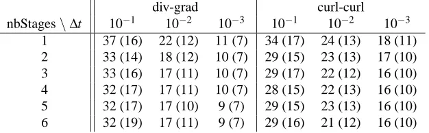
div-grad curl-curl nbStages\∆t 10−1 ₁₀−2 ₁₀−3 ₁₀−1 ₁₀−2 ₁₀−3

1 37 (16) 22 (12) 11 (7) 34 (17) 24 (13) 18 (11) 2 33 (14) 18 (12) 10 (7) 29 (15) 23 (13) 17 (10) 3 33 (16) 17 (11) 10 (7) 29 (17) 22 (12) 16 (10) 4 32 (17) 17 (11) 10 (7) 28 (15) 22 (13) 16 (10) 5 32 (17) 17 (10) 9 (7) 29 (15) 23 (13) 16 (10) 6 32 (19) 17 (11) 9 (7) 29 (16) 21 (12) 16 (10)

Table 3: Number of iterations as a function of the number of stages and the time step for a V(2,2) AMG cycle as a standalone solver and with BiCGstab acceleration (between brackets) to reach an accuracykresidualk/krhsk<10−8 for the finite element discretization of the 2D div-grad and curl-curl equations withα=β=1 using the RadauIIA IRK family on a triangular mesh containing 41624 nodes and 124075 edges on the unit square[0 1]2_{with homogeneous Dirichlet}

Tables 1 and 2 show for some fully coupled IRK and BVM methods the number of iterations as a function of the number of stages, needed to solve a 2-dimensional div-grad and curl-curl problem to a high accuracy. The accuracy is chosen high to make the differences in the results more clear. For standalone AMG, the number of itera-tions typically decreases with increasing number of stages, and the decrease becomes smaller with increasing number of stages. Table 3 shows for the RadauIIA family of IRK methods that the AMG methods converge faster for a smaller time step. Both observations confirm the results of the convergence analysis of Section 4. Similar as for scalar AMG, Krylov acceleration results in a significant reduction of the number of iterations. Note that the convergence results are similar or slightly better than for scalar AMG for the BE problem, which is equivalent to the RadauIIA case with 1 stage.

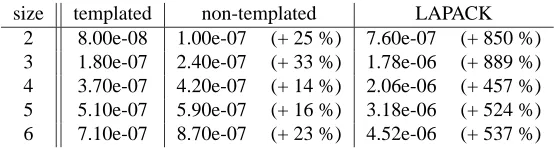
Different possible implementations of the matrix-vector products or linear solves in (25) are compared in Tables 4 and 5. The use of ad-hoc templated routines instead of the corresponding BLAS or LAPACK routines will be responsible for the main part of the reduction of the time per AMG cycle. The corresponding time reduction is of the order of magnitude of 10. Additional time reductions, achieved by the optimizations explained in Section 5, are illustrated in Figure 4.

The time needed for a fully-optimized block AMG cycle scales only quasi-linearly as a function of the number of stages for up to 6 stages (see Figure 4). This is remark-able, as the corresponding number of floating point operations scales quadratically, due to the matrix-vector products x=A−1b used to solve (25). However, thanks to their

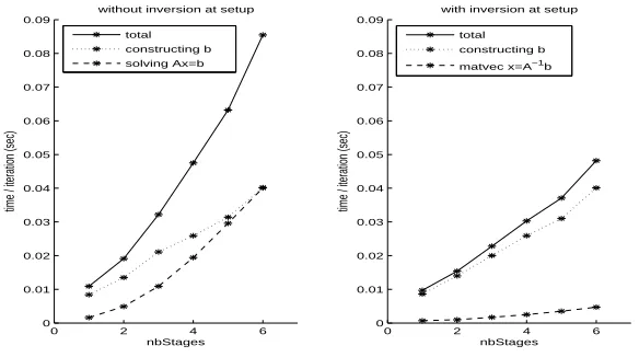
dense character, these matrix-vector products cause very little cache misses, contrary to the construction of the righthand sides of (25), which is a sparse operation. Due to these cache effects, the cost of the blocksmoother is dominated by the construction of the local righthand sides (see the right picture of Figure 5). The cost of the local dense linear solve Ax=b proves to be much higher then the cost of the

correspond-ing matrix-vector product x=A−1b, and has the same order of magnitude as the cost

of the construction of the righthand sides. Correspondingly, if the inverses of the lo-cal system matrices are not constructed and stored in the setup phase, the cost of the blocksmoother scales supralinearly (see the left picture of Figure 5).

Figure 4 shows the cost of s scalar AMG cycles as a reference. This amounts essentially to the cost of a DIRK-based AMG solver. The figure shows that for the same number of stages, the solution by AMG of the linear system arising in a fully implicit Runge-Kutta discretization is not much more expensive (typically a factor of 2 or less) than solving the sequence of s linear systems appearing in a DIRK-based time-discretization. Obviously, for the same number of stages, the order of accuracy of DIRK time discretization is significantly lower. Hence, a DIRK method will require many more (smaller) time steps than a carefully chosen fully coupled IRK method to reach a similar accuracy. Note that a more precise and quantitative comparison of DIRK versus fully implicit RK-methods would require taking into account the detailed aspects of the time step control strategy, the cost of error estimation and many more implementation heuristics. This is outside the scope of the present paper.

7

Conclusion

behav-size templated non-templated BLAS 2 7.00e-09 2.90e-08 (+ 314 %) 3.66e-07 (+ 5129 %) 3 1.80e-08 6.20e-08 (+ 244 %) 4.42e-07 (+ 2356 %) 4 3.00e-08 5.60e-08 (+ 87 %) 5.40e-07 (+ 1700%) 5 4.70e-08 1.04e-07 (+ 121 %) 5.49e-07 (+ 1068 %) 6 6.80e-08 1.62e-07 (+ 138 %) 5.80e-07 (+ 753 %)

Table 4: Average time in seconds of dense matrix-vector products using an ad-hoc templated implementation, an ad-hoc non-templated implementation and BLAS as a function of the matrix size. The compiler optimization flags -O2 and -funroll-loops are used.

size templated non-templated LAPACK 2 8.00e-08 1.00e-07 (+ 25 %) 7.60e-07 (+ 850 %) 3 1.80e-07 2.40e-07 (+ 33 %) 1.78e-06 (+ 889 %) 4 3.70e-07 4.20e-07 (+ 14 %) 2.06e-06 (+ 457 %) 5 5.10e-07 5.90e-07 (+ 16 %) 3.18e-06 (+ 524 %) 6 7.10e-07 8.70e-07 (+ 23 %) 4.52e-06 (+ 537 %)

Table 5: Average time in seconds of dense system solves using an ad-hoc templated implemen-tation, an ad-hoc non-templated implementation and LAPACK as a function of the matrix size. The compiler optimization flags -O2 and -funroll-loops are used.

ior is similar to the convergence behavior of the underlying scalar multigrid method for the backward Euler time discretization of the same problem. Also, we demonstrated that these multigrid methods offer opportunities to achieve very high cache efficiency and floating point execution rates. Considering the high order of accuracy of the time discretization methods used and the favorable convergence and timings results, the pre-sented algorithms show great promise.

References

[1] P. Bochev, C. Garasi, J. Hu, A. Robinson, and R. Tuminaro, “An improved al-gebraic multigrid method for solving Maxwell’s equations,” SIAM Journal on

Scientific Computing, vol. 25, pp. 623–642, 2003.

[2] T. Boonen, G. Deli´ege, and Vandewalle, “On algebraic multigrid methods de-rived from partition of unity nodal prolongators,” Numerical Linear Algebra with

Applications, vol. 13(2-3), no. 2-3, pp. 105–131, 2006.

[3] T. Boonen, J. Van lent, and S. Vandewalle, “Local Fourier analysis of multi-grid for the curl-curl equation,” Technical Report TW484, Katholieke Universiteit Leuven, Department of Computerscience, December 2006.

[4] A. Bossavit, Computational Electromagnetism. Boston: Academic Press, 1998.

0 2 4 6 0

0.1 0.2 0.3 0.4 0.5 0.6

number of stages

time / cycle (sec)

div−grad

0 2 4 6

0 0.5 1 1.5 2

number of stages

time / cycle (sec)

curl−curl

s x scalar AMG x=inv(A)b + row−by−row Ax=b + row−by−row x=inv(A)b + col−by−col Ax=b + col−by−col s x scalar AMG

x=inv(A)b + row−by−row Ax=b + row−by−row x=inv(A)b + col−by−col Ax=b + col−by−col

Figure 4: Average time of an AMG cycle for a 2D div-grad and curl-curl problem discretized on the same triangular mesh containing 41624 nodes and 124075 edges as a function of the number of stages, using different optimizations. “Ax=b” and “x=inv(A)b” indicate whether x in (25)

is calculated by a linear solve or by a matrix-vector product (see Section 5.3). “row-by-row” and “col-by-col” refer to the storage layout of the multivectors (see Section 5.1). The time needed for s scalar AMG cycles is indicated for comparison.

0 2 4 6

0 0.01 0.02 0.03 0.04 0.05 0.06 0.07 0.08 0.09

without inversion at setup

nbStages

time / iteration (sec)

0 2 4 6

0 0.01 0.02 0.03 0.04 0.05 0.06 0.07 0.08 0.09

with inversion at setup

nbStages

time / iteration (sec)

total constructing b solving Ax=b

total constructing b

matvec x=A−1_b

[6] L. Brugnano and D. Trigiante, Solving Differential Problems by Multistep Initial

and Boundary Value Methods, ser. Stability and Control: Theory, Methods and

Application. Amsterdam: Gordon & Breach, 1998, vol. 6.

[7] J. Butcher, Numerical methods for ordinary differential equations. Chichester: John Wiley & Sons Ltd., 2003.

[8] M. Clemens and T. Weiland, “Discrete electromagnetism with the finite integra-tion technique,” Progress in Electromagnetics Research, vol. 32, pp. 65–87, 2001.

[9] E. Hairer, S. Norsett, and G. Wanner, Solving Ordinary Differential Equations

I. Nonstiff Problems., ser. Springer Series in Comput. Mathematics. Springer-Verlag, 1993, vol. 8.

[10] E. Hairer and G. Wanner, Solving Ordinary Differential Equations II. Stiff and

Differential-Algebraic Problems., ser. Springer Series in Comput. Mathematics.

Springer-Verlag, 1996, vol. 14.

[11] R. Hiptmair, “Finite elements in computational electromagnetism,” Acta

Numer-ica, vol. 11, pp. 237–340, 2002.

[12] R. Hiptmair, “Multigrid method for Maxwell’s equations,” SIAM Journal on

Nu-merical Analysis, vol. 36, no. 1, pp. 204–255, 1999.

[13] J. Hu, R. Tuminaro, P. Bochev, C. Garasi, and A. Robinson, “Toward an h-independent algebraic multigrid method for Maxwell’s equations,” SIAM Journal

on Scientific Computing, vol. 27, no. 5, pp. 1669–1688, 2006.

[14] J. Janssen and S. Vandewalle, “Multigrid waveform relaxation on spatial finite element meshes: the discrete-time case,” SIAM J. Sci. Comput., vol. 17, no. 1, pp. 133–155, 1996.

[15] K.-A. Mardal, T. Nilssen, and G. Staff, “Order optimal preconditioners for implicit Runge-Kutta schemes applied to parabolic PDEs,” SIAM Journal on

Scientific Computing, to appear.

[16] P. Monk, Finite element methods for Maxwell’s equations. Oxford: Clarendon Press, 2003.

[17] K. Stueben, “A review of algebraic multigrid,” Journal of Computational and

Applied Mathematics, vol. 128, pp. 281–309, 2001.

[18] U. Trottenberg, C. Oosterlee, and A. Schuller, Multigrid. London: Academic Press, 2001.

[19] P. Vanek, J. Mandel, and M. Brezina, “Algebraic multigrid by smoothed aggrega-tion for second and fourth order elliptic problems,” Computing, vol. 56, no. 3, pp. 179–196, 1996.

[20] J. Van lent and S. Vandewalle, “Multigrid methods for implicit Runge-Kutta and boundary value method discretizations of parabolic PDEs,” SIAM Journal on

Scientific Computing, vol. 27, no. 1, pp. 67–92, 2005.