2009, Vol. 52, No. 2, 186-203
CONGESTION IN THE NEW BRITISH UNIVERSITIES: A FURTHER ANALYSIS
Anthony T. Flegg David O. Allen
University of the West of England
(Received February 29, 2008; Revised December 24, 2008)
Abstract The focus of this paper is on the problem of congestion, which refers to a situation where the use of a certain input has increased by so much that output has actually fallen. This problem is explored using the methodological framework proposed by F¨are et al. Annual data are examined for a sample of 41 new British universities in the period 1995/6 to 2003/4. These former polytechnics were granted university status in 1992. A widespread problem of congestion is identified. The results reveal that the order in which technical efficiency is decomposed into scale efficiency, congestion efficiency and pure technical efficiency makes a noticeable difference to the amount of congestion identified. The results also clearly indicate that an excessive number of undergraduate students is the largest single cause of congestion in these new universities. The paper concludes by considering the results from the alternative approach to the measurement of congestion formulated by Cooper et al.
Keywords: DEA, congestion, British universities
1. Introduction
The focus of this paper is on the problem of congestion, which refers to a situation where the use of a certain input has increased by so much that output has actually fallen. Congestion can be viewed as an extreme form of technical inefficiency and, as such, can be regarded as a potentially serious practical problem. Consider, for instance, the case of universities. A substantial increase in the ratio of students to academic staff has been a common experience in universities throughout the world in recent decades. As a result, the marginal product of students might have becomenegative in some universities1. The implication of this is that a
reduction in the number of students, with all other inputs (staff, buildings, etc.) held con-stant, might raise a university’s output in terms of research, consultancy and qualifications awarded, both undergraduate and postgraduate.
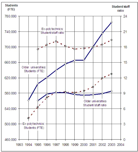
Here we explore the extent of congestion in a sample of British universities. The analysis covers the period 1995/6 to 2003/4, and our case study employs annual data pertaining to 41 former polytechnics that became universities in 1992. These new universities constitute a relatively homogeneous group, sharing a common history and facing similar opportunities and problems. In particular, as illustrated in Figure 1, they operate under much higher student : staff ratios than do the older British universities2. What is more, they typically
receive substantially less research funding per member of staff. In view of the continued under-resourcing of the former polytechnics, there are good reasons for anticipating that
1This statement presupposes that output is being measured in terms of some composite index. Marginal
products are not well defined in the case of multiple outputs.
they might be suffering from congestion.
Figure 1: Students and staff : older universities and ex-polytechnics
In an earlier study [14], we examined the problem of congestion in these new British uni-versities by using the approach proposed by Cooper et al3. Our study revealed the existence
of a widespread problem of congestion. However, a decomposition analysis produced results that we felt lacked credibility; in particular, this decomposition indicated that a sizable pro-portion of the congestion could be attributed to excessive expenditure on academic staff4.
We found it hard to understand how, in reality, academic staffing could be a congesting input.
It is of some interest, therefore, to establish whether these findings can be corroborated by the results from an alternative procedure, namely the pioneering one articulated in the monograph by F¨are, Grosskopf and Lovell in 1985 [8]5. For ease of exposition, this will be referred to hereafter as the FGL approach. A brief exposition of this method will now be offered6.
2. The FGL Approach
A useful way of attempting to explain the underlying causes of changes in technical efficiency (TE) is to employ the following decomposition [cf. 8, 170]:
T E ≡P T E ×SE×CE, (2.1)
where P T E denotes pure technical efficiency, SE denotes scale efficiency and CE denotes congestion efficiency. T E = 1 and T E < 1 represent technical efficiency and inefficiency,
3For an exposition of this approach, see [3].
4See [14, Table 6]. Corresponding results for the older universities are given in [13, Table 6]. 5Also see [1], [5] and [11].
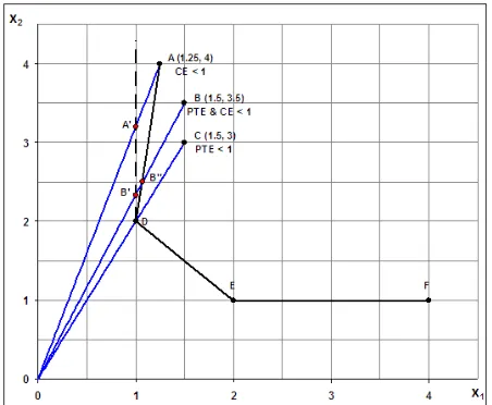
respectively. Whilst scale efficiency requires no explanation, the distinction between pure technical efficiency and congestion efficiency is worth pursuing. The simple diagrammatic example shown in Figure 2 should suffice for this purpose.
Figure 2: The FGL approach (input-oriented, CRS)
Figure 2 shows six decision-making units (DMUs), each producing an output of y = 1, using two inputs,x1 and x2. This example assumes constant returns to scale (CRS), so that
SE = 1, and makes use of aninput-orientedapproach. DMUs D and E are clearly technically efficient, whereas C is inefficient. In terms of identity (2.1) above,T E =P T E = 2/3 for C. Less obviously, F would also be deemed to be technically efficient under the FGL approach. Here the slack inx1of two units would be disregarded on the basis that these units werefreely disposable, i.e. could be disposed of at no opportunity cost. Indeed, F¨are and Grosskopf [6, 32–33] argue that, given positive input prices, non-zero slack is akin to allocative rather than technical inefficiency.
The classification of DMUs A and B is both more complicated and more controversial. With respect to A, the FGL analysis would proceed along the following lines. Because A is on the isoquant for y = 1, this DMU would be regarded as exhibiting no pure technical inefficiency (P T E = 1). However, it would be deemed to be suffering from congestion. A’s CE score, as measured by the ratio OA′/OA, would equal 0.8. Its T E score would also equal 0.8, the product of P T E = 1 and CE = 0.8. Congestion would arise owing to the difference between the upward-sloping isoquant segment DA, which is assumed to exhibit
weak disposability, and the hypothetical vertical dashed line emanating from D, which is assumed to exhibit strong (or free) disposability. By moving to point A′, and thereby eliminating its congestion, A could attain T E = 1. By contrast, DMU B would exhibit both pure technical inefficiency and congestion under the FGL approach. For B, P T E =
OB′′/OB ≈0.714 and CE =OB′/OB′′ ≈0.933, so thatT E = 2/3≈0.714×0.9337.
An issue that needs to be addressed when applying the FGL approach is that the val-ues of SE and CE in the identity (2.1) above will depend upon the order in which the decomposition is carried out, although T E, P T E and the product SE ×CE will not be affected. In their earlier work, F¨are et al. assumed strong disposability when measuring scale effects, and only then considered the possibility of congestion. In other words, they
computed SE as (ϕ|C, S)/(ϕ|V, S), where C and V denote constant and variable returns to scale, respectively, S denotes strong disposability, and ϕ is the efficiency score. Having calculatedSE in this way, they computedCE as (ϕ|V, S)/(ϕ|V, W), whereW denotes weak disposability8. However, F¨are and Grosskopf [7] have highlighted the difficulty of
discrimi-nating between scale inefficiency and congestion; they point out that different answers will be obtained depending on the order in which T E is decomposed. Therefore, where con-gestion is anticipated on a priori grounds, they recommend that one should specify CRS rather than VRS (variable returns to scale) technology when measuring congestion. Under CRS technology, CE would be computed first as (ϕ|C, S)/(ϕ|C, W), with SE computed thereafter as (ϕ|C, W)/(ϕ|V, W)9.
Another important issue concerns the distinction between input and output congestion. Input congestion, which is the focus of this paper, refers to a situation where the overuse of one or more inputs has caused a fall in output. Output congestion, on the other hand, refers to ‘the loss of potential output due to the lack of strong disposability of outputs’ [9, 110]. In such cases, a subset of outputs is obstructing the production of the remaining output(s). For instance, one of the outputs may be an undesirable by-product of joint production, e.g. air pollution associated with the generation of electricity (cf. [10]). If, owing to environmental restrictions, a power station has to use scarce resources to abate its pollution, then pollution will no longer be a freely disposable output and should be regarded instead as weakly disposable, i.e. congesting. However, in the case of universities, it seems reasonable to assume that all outputs are strongly disposable. Consider, for instance, a university that produces three outputs: research and consultancy (y1), undergraduate degrees (y2) and
postgraduate degrees (y3). The university is likely to treat all three outputs as desirable.
Now suppose that the university wanted to cut its output of, say,y3. Fory3 to be held to be
a congesting output, the cut in y3 would need to be accompanied by either (i) a reduction
in y1 or in y2 or in both or (ii) an increase in one or more inputs, e.g. extra academic staff
[cf. 9, 43]. There is no compelling reason to suppose that any of these changes would be needed. In short, it seems reasonable to posit strong disposability of all outputs.
A final issue concerns the orientationof the model. Here it should be noted that, in the current version ofOnFront, the software supporting the FGL approach, congestion of inputs is measured using an input-oriented approach, whereas congestion of outputs is captured via an output-oriented approach10.
In view of the above arguments, we will be employing an input-oriented variant of the FGL approach, with CRS as the underlying technology, to compute CE and SE scores for each university. This approach is consistent with the earlier discussion surrounding Figure 2. However, for comparative purposes, we will also present results based on VRS.
3. DEA Model
Following previous research (see [12], [13] and [14]), our DEA model presumes that a univer-sity’s output can be measured by the benefits it provides in terms of teaching and research. These aspects of a university’s activities are captured here via the following variables:
• the total number of undergraduate qualifications awarded (y1);
• the total number of postgraduate qualifications awarded (y2);
8See, for example, [1]. A more recent example is [12].
9See Appendix A for a formal explanation of the congestion models.
10We are grateful to Pontus Roos, of the Institute of Applied Economics in Sweden, for clarifying this issue
• income from research grants and contracts in£ thousands (y3)11.
Again following previous research, the inputs used in producing the above-mentioned out-puts are assumed to be:
• the number of full-time equivalent undergraduate students (x1);
• the number of full-time equivalent postgraduate students (x2);
• academic staff expenditure in £ thousands (x3);
• other expenditure in £ thousands (x4).
Although a detailed rationale for the outputs and inputs listed above is given in [14], along with sources of data and other details, certain facets of our model are worth exploring here. A notable feature of this model is that the number of students is treated as an input, whereas the number of qualifications obtained is regarded as an output. Here it might be objected that, because students are the recipients of the educational services provided by a university, the number of students should be classified as an output rather than an input. However, that would not take into account how successful a university was in terms of producing qualified students. Indeed, we believe that our choice of inputs and outputs is in accord with the usual notions of productivity underlying DEA.
Another point worth clarifying is our treatment of undergraduate students who fail to complete a full bachelors degree but nonetheless successfully complete their first or second year. Normally, such students are awarded an intermediate qualification to recognize their achievements: a Certificate of Higher Education at the end of Year 1 and a Diploma of Higher Education at the end of Year 212. We have included such awards in our output variable y1. However, a possible shortcoming of this variable is the fact that, in the present
study, all undergraduate qualifications are weighted equally, regardless of the length of study required or the class of degree obtained.
4. Decomposing Technical Efficiency
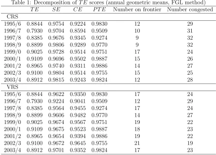
To shed some light on the causes of annual fluctuations in technical efficiency, we used the FGL procedure to decompose theT E scores for individual universities. Then, to summarize the results for each year, geometric means were taken, so that T E = P T E×SE×CE13. Two alternative assumptions were made regarding the underlying technology, namely CRS and VRS. The outcomes are displayed in Table 1 and illustrated in Figures 3–5.
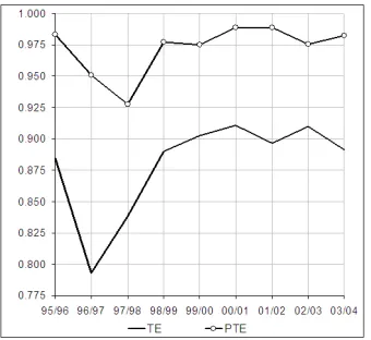
The behaviour of P T E, as depicted in Figure 3, will be considered first. It should be noted that this component ofT Eis unaffected by the choice of technology. Figure 3 reveals a relatively stable pattern inP T E after 1998/9. There is also no obvious relationship between the fluctuations inT E and P T E.
Figures 4 and 5 examine the effects of switching between CRS and VRS. It is evident that positing CRS rather than VRS technology yields rather more congestion (lower CE) and rather less scale inefficiency (higher SE). It is evident that there is a relationship between the fluctuations in the mean CE and T E scores. This is true for both CRS and VRS. In particular, the sharp fall in T E in 1996/7 and modest rise in 2002/3 are obviously
11It is acknowledged that income from research grants and contracts could be viewed as an intermediate
input rather than as an output. However, the use of this proxy for research output was dictated by the lack of annual data for alternative measures. For further discussion, see [14, 55].
12Some students regard such certificates and diplomas as their preferred final qualification rather than as a
default qualification.
13Note that the product SE×CE is unaffected by the order of decomposition. We tried weighting the
Table 1: Decomposition of T E scores (annual geometric means, FGL method)
T E SE CE P T E Number on frontier Number congested
CRS
1995/6 0.8844 0.9754 0.9224 0.9830 12 29 1996/7 0.7930 0.9704 0.8594 0.9509 10 31 1997/8 0.8385 0.9676 0.9345 0.9274 9 32 1998/9 0.8899 0.9806 0.9289 0.9770 9 32 1999/0 0.9025 0.9728 0.9514 0.9751 17 24 2000/1 0.9109 0.9696 0.9502 0.9887 15 26 2001/2 0.8965 0.9740 0.9311 0.9886 14 27 2002/3 0.9100 0.9804 0.9514 0.9755 15 25 2003/4 0.8912 0.9815 0.9243 0.9824 12 28
VRS
1995/6 0.8844 0.9622 0.9350 0.9830 17 24 1996/7 0.7930 0.9224 0.9041 0.9509 12 29 1997/8 0.8385 0.9564 0.9455 0.9274 17 24 1998/9 0.8899 0.9606 0.9482 0.9770 14 27 1999/0 0.9025 0.9674 0.9567 0.9751 19 22 2000/1 0.9109 0.9675 0.9523 0.9887 18 23 2001/2 0.8965 0.9654 0.9394 0.9886 19 22 2002/3 0.9100 0.9672 0.9645 0.9755 21 19 2003/4 0.8912 0.9701 0.9352 0.9824 17 23
associated with the corresponding movements in CE. However, in the case of the VRS results, the decline in CE in 1996/7 cannot wholly explain the precipitous fall in T E in that year. This is because the rise in congestion was reinforced by greater scale inefficiency. There was also a fall in P T E in 1996/7.
5. Causes of Congestion
Having examined the trends in congestion, we can now attempt to unravel its underlying causes. Hitherto, in calculating the CE scores for individual universities, it has been as-sumed that all four inputs were either strongly (S) or weakly (W) disposable, where weak disposability allows for the possibility of congestion. This comparison can be symbolized as SSSS versus WWWW. However, there are a priori grounds for questioning whether it is sensible to posit weak disposability with respect to academic staff expenditure (x3) and
other expenditure (x4). In particular, why should a rise in each type of expenditure cause
a fall in output? By contrast, a rise in the number of full-time equivalent undergraduates (x1) or postgraduates (x2), with academic staffing and other resources held constant, could
well lead to a fall in output in terms of research and consultancy. This is because the extra students would be competing for scarce staff time. There would be additional costs in terms of assessment, supervision, etc. On the other hand, extra postgraduate students could be helpful in terms of stimulating research output. As regards undergraduate students, output in terms of qualifications awarded could decline with an increase in the number of under-graduates because staff would be unable to devote the same amount of time to each student as before.
Figure 3: Trends in mean T E and P T E Figure 4: Trends in mean T E and SE
Figure 5: Trends in mean T E and CE
of strong disposability for each input in turn. The outcomes of this process are presented in Table 2 and illustrated in Figures 6–7. For ease of interpretation, the results have been expressed in terms of congestion scores, rather than congestion efficiency (CE) scores. For example, the CRS-based congestion score of 0.0757 for 2003/4 is simply 1–0.9243, where 0.9243 is the geometric mean of the individualCE scores for that year (see Table 1). In the diagrams, the top lines show the congestion scores when all inputs are examined for possible congestion (WWWW), whereas the bottom lines show the scores when only undergraduates are considered (WSSS).
One aspect of the procedure requires some explanation, namely the order in which the assumption of strong disposability was relaxed for the four inputs. There are, in fact, 14 possible ways in which one could relax this assumption. However, in order to simplify this process, we started with undergraduates (WSSS) because we believed that this input was the one most likely to be congested. We then added postgraduates (WWSS), academic staff expenditure (WWWS) and, finally, other expenditure (WWWW). This ordering is, of course, somewhat arbitrary and, for this reason, we carry out a sensitivity analysis in the next section.
[image:7.595.104.274.75.231.2] [image:7.595.338.509.78.226.2]Table 2: Congestion scores under different assumptions as regards disposability (FGL method)
Inputs being examined for congestion
x1 x1, x2 x1, x2, x3 all
CRS
1995/6 0.0349 0.0453 0.0650 0.0776 1996/7 0.0616 0.0800 0.1277 0.1406 1997/8 0.0228 0.0459 0.0574 0.0655 1998/9 0.0420 0.0525 0.0677 0.0711 1999/0 0.0308 0.0334 0.0475 0.0486 2000/1 0.0336 0.0419 0.0473 0.0498 2001/2 0.0411 0.0521 0.0560 0.0689 2002/3 0.0351 0.0410 0.0432 0.0486 2003/4 0.0514 0.0578 0.0751 0.0757
VRS
1995/6 0.0314 0.0393 0.0559 0.0650 1996/7 0.0482 0.0651 0.0898 0.0959 1997/8 0.0206 0.0427 0.0486 0.0545 1998/9 0.0332 0.0382 0.0503 0.0518 1999/0 0.0234 0.0300 0.0401 0.0433 2000/1 0.0282 0.0385 0.0458 0.0477 2001/2 0.0379 0.0478 0.0539 0.0606 2002/3 0.0259 0.0279 0.0308 0.0355 2003/4 0.0395 0.0486 0.0635 0.0648
congestion. Also as expected, postgraduates appear to play a significant role in generating congestion, albeit a much smaller role than that of undergraduates. Congestion was not an-ticipated in the case of other expenditure and here the graphs show only a modest amount in most years14. What is most surprising, however, is the significant amount of congestion attributed to academic staff. This is especially noticeable in 1996/7.
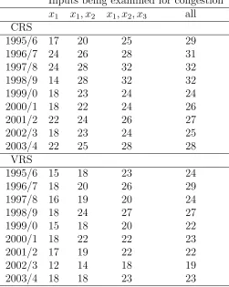
The rise in the congestion scores when an extra input is considered for possible congestion occurs for two reasons: (i) a rise in the scores of some existing congested universities and (ii) the identification of newly congested universities. This second effect is illustrated in Table 3.
The unexpected finding that congestion in the ex-polytechnics was, to a material extent, due to excessive expenditure on academic staff warrants some discussion. Intuitively, it does seem improbable that such overspending would have reduced the output of congested universities in terms of income from research grants and contracts, and the number of under-graduate and postunder-graduate awards. However, a possible explanation is that academic staff expenditure might be capturing the effects of an omitted variable such as the effectiveness of management15. It is also conceivable that the apparent existence of ‘surplus’ academic staff
in the congested universities could be indicative of institutional inefficiency in a broader sense. A final possibility is that the results might reflect heterogeneity of both staff and
14For some years, e.g. 1999/0 and 2003/4, the congestion of other expenditure is hard to discern from the
graphs but Table 2 shows that it did exist.
[image:8.595.179.431.118.437.2]Figure 6: Components of overall congestion score: CRS
Figure 7: Components of overall congestion score: VRS
students. For example, universities are likely to differ in terms of the entry qualifications of their students and the expertise of their academic staff.
Whilst the congesting role attributed to ‘other expenditure’ is modest, it is just as per-plexing. What this finding indicates is that, after a certain point, extra spending actually re-duced congested universities’ output. However, ‘other expenditure’ is a very broadly defined input variable, comprising expenditure on academic cost centres, academic services, admin-istration and central services, premises, residences and catering, and on research grants and contracts, and it is conceivable that one or more of these components could be congest-ing. For instance, by creating an unwieldy bureaucracy, overspending on administration might reduce a university’s efficiency and hence output in terms of research and qualifi-cations awarded. It is also possible that a rise in the proportion of ‘other expenditure’ devoted to research could reduce the number of undergraduate and postgraduate qualifica-tions awarded, if it meant lower spending on teaching-related activities. Thus higher total expenditure could lead to a rise in some outputs but a fall in others, with the net impact uncertain.
6. Alternative Approaches
In an earlier study [14], we examined the problem of congestion in the former polytechnics by using the approach proposed by Cooper, Gu and Li [4]. For ease of exposition, this method is referred to here as the CGL approach. It is worth exploring how far these earlier CGL-based results differ from those obtained here for the FGL approach. Of particular importance are any differences in: (i) the proportion of congestion attributable to each input and (ii) the number of universities identified as being congested.
The CGL procedure differs in several respects from the FGL approach. Most notably, it is a non-radial method based on VRS, whereas the FGL approach is a radial method. Another key difference is the fact that F¨are et al. impose the restriction of weak disposability, whereas Cooper et al. do not. The CGL approach also employs an output orientation, in contrast to the input orientation used in the FGL procedure. With the CGL approach, the overall congestion score for each universityj is computed via the following formula:
Table 3: Number of congested universities under different assumptions as regards dispos-ability (FGL method)
Inputs being examined for congestion
x1 x1, x2 x1, x2, x3 all
CRS
1995/6 17 20 25 29
1996/7 24 26 28 31
1997/8 24 28 32 32
1998/9 14 28 32 32
1999/0 18 23 24 24
2000/1 18 22 24 26
2001/2 22 24 26 27
2002/3 18 23 24 25
2003/4 22 25 28 28
VRS
1995/6 15 18 23 24
1996/7 18 20 26 29
1997/8 16 19 20 24
1998/9 18 24 27 27
1999/0 15 18 20 22
2000/1 18 22 22 23
2001/2 17 19 22 22
2002/3 12 14 18 19
2003/4 18 18 23 23
where sij is the BCC slack for input i and xij is the quantity used of input i16.
For comparative purposes, it is necessary to work out what proportion of the overall congestion score can be attributed to each input under each approach. With the CGL ap-proach, the percentage share for inputiequals 100(sij/xij)/4Cj. The necessary calculations
are reported in [14, Table 6]. Unfortunately, with the FGL procedure, there is no unique way of calculating the contribution of each input.
An obvious way of measuring the contributions under the FGL approach would be to use the figures in Table 2. For example, we could use the CRS results for 2003/4 to calculate the shares of the four inputs as follows:
share of x1 = (0.0514/0.0757)×100 = 67.9%
share of x2 ={(0.0578−0.0514)/0.0757} ×100 = 8.4%
share of x3 ={(0.0751−0.0578)/0.0757} ×100 = 22.9%
share of x4 ={(0.0757−0.0751)/0.0757} ×100 = 0.8%
However, as explained in Appendix B, this method can yield misleading results, with the outcome dependent upon the order in which strong disposability is relaxed. Hence an alternative approach was also pursued.
This alternative procedure involved a reversal of the order in which strong disposability was relaxed, whereby we began with x4 (rather than x1) and then added x3, x2 and x1 in
turn. Thus we started with the input we believed to be the least likely source of congestion
16This formula presupposes that no DMU on the BCC frontier has non-zero slack. This is not a restrictive
and ended with the one we thought was most likely to be congesting. The results were as follows:
share of x4 = (0.0050/0.0757)×100 = 6.6%
share of x3 ={(0.0305−0.0050)/0.0757} ×100 = 33.6%
share of x2 ={(0.0364−0.0305)/0.0757} ×100 = 7.8%
share of x1 ={(0.0757−0.0364)/0.0757} ×100 = 52.0%
It is evident that reversing the order in which strong disposability is relaxed does alter the outcomes considerably. In particular, the share of x1 (undergraduates) is now much lower,
whereas that of x3 (academic staff) is much higher. The share of x4 (other expenditure)
is also noticeably higher. In fact, x2 (postgraduates) is the only input to exhibit a stable
share.
The above findings suggest that the original method is likely to overstate the shares of
x1 and x2, yet understate those of x3 and x4, whereas the alternative method is apt to do
the opposite17. To circumvent this problem, we decided to average the results from the two
[image:11.595.214.394.343.671.2]methods. The outcomes are presented in Table 4.
Table 4: Percentage contribution of each input to the overall congestion score (FGL method)
x1 x2 x3 x4
CRS
1995/6 37.6 11.1 30.6 20.8 1996/7 33.1 8.4 44.1 14.4 1997/8 25.2 29.3 31.6 14.0 1998/9 46.3 12.3 37.4 4.0 1999/0 54.6 4.5 34.3 6.6 2000/1 58.7 14.7 15.1 11.4 2001/2 49.1 14.8 9.2 26.9 2002/3 64.2 14.0 5.5 16.4 2003/4 60.0 8.1 28.3 3.7
Mean 47.6 13.0 26.2 13.1 VRS
1995/6 35.5 8.9 30.8 24.9 1996/7 40.5 10.5 33.3 15.7 1997/8 23.4 32.6 28.3 15.7 1998/9 52.1 8.0 34.3 5.6 1999/0 45.5 12.5 31.8 10.2 2000/1 53.1 15.7 19.7 11.5 2001/2 42.9 18.3 12.3 26.5 2002/3 61.1 7.1 6.3 25.5 2003/4 51.8 13.2 27.4 7.7
Mean 45.1 14.1 24.9 15.9
Table 4 confirms the earlier finding (illustrated in Figures 6–7) that having too many
17Discriminating between x
3 (academic staff expenditure) and x4 (other expenditure) is complicated by
the existence of a fairly high correlation between these two inputs; this correlation ranged from 0.782 to 0.838 during the sample period. There was also a fairly strong correlation between x3 and both x1
(undergraduates) andx2(postgraduates). By contrast,x1andx2were more modestly correlated with each
undergraduates is by far the largest single cause of congestion. On average, based on the VRS results, undergraduates contributed 45.1% to congestion scores during the period under review. This is a much larger figure than the 33.3% we obtained from our CGL analysis. By contrast, for postgraduates, the mean contribution of 14.1% shown in Table 4 falls well short of the 20.9% we found using the CGL approach. However, the combined average share of students (undergraduates plus postgraduates) is 59.2% for the FGL method, compared with 54.2% for the CGL method. In this sense, the findings reported here are a little more credible than those we obtained previously. It is interesting that the two approaches yield fairly similar mean shares for academic staff expenditure (FGL: 24.9%, CGL: 26.0%), although the gap is larger for other expenditure (15.9% versus 19.8%).
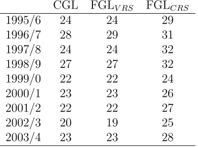
Table 5: Number of congested universities identified under different approaches CGL FGLV RS FGLCRS
1995/6 24 24 29
1996/7 28 29 31
1997/8 24 24 32
1998/9 27 27 32
1999/0 22 22 24
2000/1 23 23 26
2001/2 22 22 27
2002/3 20 19 25
2003/4 23 23 28
Table 5 shows the number of congested universities under each approach. What is most striking about these results is that an assumption of CRS considerably increases the number of universities held to be congested under the FGL procedure. However, when VRS is assumed, the CGL and FGL methods yield almost identical results in terms of the number of congested universities. It should be noted, though, that this does not mean that the amount of congestion identified by each method will be the same. This is because the formulae used to measure congestion are very different, as is the orientation employed. It is worth mentioning that the new approach to measuring congestion proposed by Tone and Sahoo [17] produced almost identical results to the CGL procedure in terms of classifying universities as congested or uncongested. This finding can be explained by the fact that this new method also uses the BCC model as its starting point.
7. Disaggregated Results
Appendix C displays a set of results for 40 individual universities in 2003/418. These results illustrate the effects of changing the order of decomposition. It should be noted that:
T E ≡P T E×SEV RS×(1−CF,V RS)≡P T E×SECRS ×(1−CF,CRS), (7.1)
whereCF,V RS is the FGL congestion score calculated on the assumption of VRS technology
and SEV RS is the corresponding scale efficiency score. SECRS and CF,CRS are defined
analogously. For comparison, the congestion score, CC, from the CGL method is also
shown.
[image:12.595.208.404.261.406.2]The individual results reveal a diversity that is hidden when looking at annual means. A good example is Thames Valley, which has the lowest T E score in the sample. This score suggests that this university could have produced the same output with only 51% of the inputs actually employed in 2003/4, if it had been fully efficient. As to the causes of this technical inefficiency, F¨are et al. would regard Thames Valley as being chronically congested, whereas Cooper et al. would find only a moderate amount of congestion. Also of interest are Thames Valley’sSE scores, which show that the choice of technology has some bearing on the apparent causes of inefficiency. Here, if we assume CRS, we find no scale inefficiency, whereas an assumption of VRS yields a substantial amount of scale inefficiency (SEV RS = 0.8437).
Robert Gordon is another university worth examining. It has T E = SEV RS = 0.9101.
The fact that its T E and SEV RS scores are identical shows that it was operating on the
VRS frontier. Thus any congestion would be ruled out. The same outcome occurs under CGL approach. However, under the CRS-based version of the FGL procedure, congestion is possible and, indeed, Robert Gordon hasCF,CRS = 0.0899. There are five other universities
in a similar situation.
As a final example, consider West of England. This is interesting insofar as it is one of only six universities exhibiting pure technical inefficiency. What is more, one can see that the presence of this type of inefficiency is clearly the predominant factor behind this university’s relatively lowT E score. Indeed, the FGL results indicate relatively high scale efficiency and negligible congestion, regardless of whether one posits CRS or VRS technology. By contrast, the CGL procedure records a modest amount of congestion.
Some interesting information can be gleaned from the congestion scores. For instance, one can see thatCF,V RS and CC generate exactly the same set of congested universities, yet
the amounts of congestion identified by the two methods are very different. On average, the VRS-based version of the FGL approach indicates congestion of 6.0% of inputs, whereas the CGL approach records congestion of only 3.25%. This divergence is a consequence of the different assumptions underlying the two methods, the difference in the orientation employed and dissimilarities in the formulae used to measure congestion. It is worth noting too that the mean amount of congestion rises to 7.0% of inputs if the CRS-based version of the FGL approach is employed. What is more, the number of universities held to be congested rises from 23 to 28. The differences in the congestion measures are reflected in the dissimilarity of the rankings shown in the table.
8. Choice of Approach
The last two sections have highlighted the point that the alternative approaches of F¨are et al. and Cooper et al. are apt to yield very different findings with respect to congestion. This raises the question as to which approach, if any, should be preferred. One way of addressing this issue would be to examine their theoretical properties but this is complicated by the fact that each approach has particular merits and demerits. For instance, the FGL approach has firm theoretical foundations, yet it might be argued that the axiom of weak disposability is too restrictive in the sense that not all cases where there is an inverse relationship between inputs and outputs are held to represent congestion. By contrast, the CGL approach encompasses all such cases, yet a weakness of this approach is the fact that the CGL measure of congestion does not have an explicit theoretical basis19.
19For a more detailed discussion of the pros and cons of alternative approaches to measuring congestion,
The approaches also differ in terms of their underlying aims. Here Cherchye et al. [2, 77–78] observe that the original aim of the FGL procedure was not to measure the amount of congestion per se but instead to assess the impact, if any, of congestion on the overall technical efficiency of a particular DMU. In contrast, the CGL method was specifically designed to measure congestion. Thus, if one’s aim is to measure the impact of congestion on the TE score of a given DMU, then it seems logical to opt for the FGL approach. If, instead, one’s aim is to measure the amount of congestion, then the CGL method might be preferred.
Nevertheless, the FGL procedure does have a particular advantage over the CGL proce-dure in the present context: one can choose which inputs to examine for possible congestion. This is important given the doubts expressed earlier as to whether it is reasonable to ex-pect academic staff expenditure (x3) and other expenditure (x4) to be congesting inputs.
Another point in favour of the FGL procedure is the fact that, in comparison with the CGL procedure, a somewhat smaller proportion of the overall congestion score was attributed to these two inputs.
If we were to rule out the possibility ofx3 andx4 being congested — by imposing strong
disposability — then the inefficiency hitherto attributed to congestion would need to be reclassified as scale inefficiency or as pure technical inefficiency or as both. Hence, in the inequalityT E ≡P T E×SE×CE, CE would rise andP T E×SE would fall. To illustrate, consider the VRS-based results for 2003/4 shown in Table 2. By assuming weak disposability for x1 and x2 but strong disposability forx3 and x4, we would get a mean congestion score
for that year of 0.0486, aCE of 0.9514 and aP T E of 0.9656. By contrast, if all inputs were assumed to be weakly disposable, the respective figures would be 0.0648, 0.9352 and 0.9824.
9. Conclusion
This study has examined the extent of ‘congestion’ in a sample of 41 former British poly-technics that became universities in 1992, using annual data for the period 1995/6 to 2003/4. Congestion is a problem that can occur when a certain input is overused to such an extent that output actually falls. We felt that there were good reasons for anticipating congestion in the case of these new universities because they have far higher student : staff ratios than do the older British universities, along with much lower research funding per member of staff20.
Congestion was measured using the methodology developed by F¨are, Grosskopf and Lovell (FGL). Two versions of this approach were considered: one assumed constant returns to scale (CRS), while the other assumed variable returns to scale (VRS). Both versions indicated a widespread problem of congestion in the former polytechnics. In addition, for comparative purposes, the alternative approach to the measurement of congestion proposed by Cooper, Gu and Li (CGL) was also considered.
The different measures of congestion generated contrasting results in terms of the severity of congestion. The CRS-based version of the FGL approach consistently produced the highest congestion scores. For instance, the mean score for the 40 universities in 2003/4 was 7.0%, in excess of the 6.0% for the VRS-based variant of the FGL procedure and well above the 3.25% for the CGL method21.
The underlying causes of congestion were explored via a decomposition analysis based
20The student : staff ratio in the ex-polytechnics rose from 17.5 to 19.3 between 1995/6 and 2003/4, whereas
the ratio in the older universities rose from 7.5 to 9.9.
on the FGL procedure. This revealed that an excessive number of undergraduates was by far the biggest single cause of congestion in the former polytechnics during the period under review. For instance, the CRS-based variant of the FGL approach indicated that such students accounted for 60.0%, on average, of the overall amount of congestion observed in 2003/4. Less credible was the finding that excessive expenditure on academic staff was also a major cause of congestion in the former polytechnics! Here the results recorded a share of 28.3% in 2003/4. By contrast, the results signified that postgraduates (8.1%) and ‘other expenditure’ (3.7%) had a much smaller role in generating congestion in that year.
It is worth noting that, when compared with the FGL results, the CGL procedure gave very different shares in 2003/4 for undergraduates (42.3% versus 60.0%), postgraduates (12.3% versus 8.1%) and ‘other expenditure’ (16.0% versus 3.7%), yet a very similar figure for academic staff expenditure (29.5% versus 28.3%) [14, Table 6].
The contrasting findings from the FGL and CGL procedures raise the question as to which set of results, if any, should be preferred. There is no straightforward answer to this question but we noted that the FGL procedure was the logical choice in cases where one wished to assess the impact of congestion on the overall technical efficiency of a particular university. The use of this procedure also made it possible to rule outa prioriany implausible cases of apparent congestion and to reclassify these as scale inefficiency or as pure technical inefficiency or as both.
Nevertheless, it is of concern that both procedures indicated a sizable amount of conges-tion due to excessive expenditure on academic staff. This finding is clearly worthy of further investigation, as it may reflect shortcomings in the DEA models or in the data used to run these models. In particular, the apparent academic overstaffing may reflect institutional inefficiency in a broader sense.
In terms of implementing the findings of this study, one important caveat needs to be stated: it may well be much easier to comprehend the causes of congestion than to realize the potential gains in output from eliminating such congestion. As regards the different results generated by the alternative methods of measuring congestion, one should not lose sight of the fact that the CGL procedure (which assumes VRS) and the VRS-based variant of the FGL method almost invariably identified the same universities as being congested. Where they differed was in terms of the severity of congestion in the universities affected. Nevertheless, it is clear that one is likely to find more ‘congestion’ with a CRS-based model than with a VRS-based model.
Acknowledgements
An earlier version of this paper was presented at an international DEA symposium held at Seikei University, Tokyo in February 2008. Thanks are due to the Japan Society for Promotion of Sciences, and to Hiroshi Morita and Kaoru Tone, for making this possible. We are also very grateful to the two anonymous referees for their detailed and constructive comments, which led to many improvements in the paper. Finally, we would like to thank Rolf F¨are for reading our paper prior to its submission.
References
[1] P. Byrnes, R. F¨are, and S. Grosskopf: Measuring productive efficiency: an application to Illinois strip mines. Management Science, 30 (1984), 671–681.
132 (2001), 75–80.
[3] W.W. Cooper, H. Deng, L.M. Seiford, and J. Zhu: Congestion: its identification and management with DEA. In W.W. Cooper, L.M. Seiford and J. Zhu J. (eds.): Handbook on Data Envelopment Analysis (Kluwer, Boston, 2004), 177–201.
[4] W.W. Cooper, B. Gu, and S. Li: Comparisons and evaluations of alternative approaches to the treatment of congestion in DEA.European Journal of Operational Research,132
(2001), 62–74.
[5] R. F¨are and S. Grosskopf: Measuring congestion in production. Zeitschrift f¨ur Na-tional¨okonomie, 43 (1983), 257–271.
[6] R. F¨are and S. Grosskopf: Slacks and congestion: a comment.Socio-Economic Planning Sciences,34 (2000), 27–33.
[7] R. F¨are and S. Grosskopf: Research note: decomposing technical efficiency with care.
Management Science,46 (2000), 167–168.
[8] R. F¨are, S. Grosskopf, and C.A.K. Lovell: The Measurement of Efficiency of Production
(Kluwer-Nijhoff, Boston, 1985).
[9] R. F¨are, S. Grosskopf, and C.A.K. Lovell: Production Frontiers(Cambridge University Press, Cambridge, 1994).
[10] R. F¨are, S. Grosskopf, C.A.K. Lovell, and C. Pasurka: Multilateral productivity com-parisons when some outputs are undesirable: a non-parametric approach. Review of Economics and Statistics, 71 (1989), 90–98.
[11] R. F¨are and L. Svensson: Congestion of production factors. Econometrica, 48 (1980), 1745–1753.
[12] A.T. Flegg, D.O. Allen, K. Field, and T.W. Thurlow: Measuring the efficiency of British universities: a multi-period data envelopment analysis. Education Economics,
12 (2004), 231–249.
[13] A.T. Flegg and D.O. Allen: Does expansion cause congestion? The case of the older British universities, 1994–2004. Education Economics,15 (2007), 75–102.
[14] A.T. Flegg and D.O. Allen: Using Cooper’s approach to explore the extent of congestion in the new British universities. Economic Issues, 12-2(2007), 47–81.
[15] A.T. Flegg and D.O. Allen: Congestion in the Chinese automobile and textile industries revisited. Socio-Economic Planning Sciences,43 (2009), 177–191.
[16] S.C. Ray: Data Envelopment Analysis: Theory and Techniques for Economics and Operations Research (Cambridge University Press, Cambridge, 2004).
[17] K. Tone and B.K. Sahoo: Degree of scale economies and congestion: a unified DEA approach. European Journal of Operational Research,158 (2004), 755–772.
Appendix A. Congestion models
Assuming weak disposability of inputs and VRS, the FGL linear programming problem for each DMU k can be specified as follows [cf. 16, 178]:
Minimize θ (A.1)
subject to ∑
j
λjxij = (α)θxik, i= 1,2, . . . , m (A.2)
∑
j
λjyrj ≥yrk, r = 1,2, . . . , s (A.3)
∑
j
λj ≥0, j = 1,2, . . . , n (A.5)
where xij and yrj are the quantities of input i and output r produced by DMU j, and
the λj are a set of weights with values to be determined. α in (A.2) can be set equal to
unity without affecting the optimal value of θ [16, 178]. The above model differs from the standard BCC input-oriented model only insofar as the input constraints (A.2) are expressed as equations rather than as weak inequalities [16, 178]. Removing the convexity constraint ∑
jλj = 1 would mean reverting to CRS.
Appendix B. Calculating the contribution of each input to the overall conges-tion score
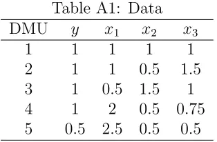
[image:17.595.227.384.298.401.2]Consider the following example proposed by one of the anonymous referees.
Table A1: Data DMU y x1 x2 x3
1 1 1 1 1
2 1 1 0.5 1.5 3 1 0.5 1.5 1 4 1 2 0.5 0.75 5 0.5 2.5 0.5 0.5
[image:17.595.84.526.458.597.2]The outcomes are displayed in Table A2.
Table A2: CRS-based results under different assumptions regarding disposability Model Efficiency score DMU 5 DMU 5 Share of congestion
due to each input (%) DMUs 1–4 DMU 5 CE 1−CE x1 x2 x3
1: SSS 1 0.75 1 0
2: WSS 1 1 0.75 0.25 100
3: WWS 1 1 0.75 0.25 100 0
4: WWW 1 1 0.75 0.25 100 0 0
5: SSW 1 0.8 ˙3 0.9 0.1 40
6: SWW 1 0.8 ˙3 0.9 0.1 60 0 40
Note: SSS denotes that all three inputs are held to be strongly disposable (i.e. uncon-gested), WSS denotes that x1 is assumed to be weakly disposable (i.e. potentially
con-gested), whereas x2 and x3 are assumed to be strongly disposable, and so on.
Table A2 demonstrates that the share of overall congestion (i.e. the outcome under WWW) attributable to each input depends on the order in which the assumption of strong disposability is relaxed. For instance, if we start with Model 2, we find that 100% of the congestion is due to x1. However, if we start with Model 5, we find that 40% of the
congestion is due to x3 and only 60% to x1. One way of dealing with these conflicting
outcomes would be to average the results, so that the share of x1 would be deemed to be
Appendix C. Individual results for 2003/4
University Weight T E rank SEV RS SECRS P T E CF,CRS rank CF,V RS rank CC rank
Abertay Dundee 0.007 1 1 1 1 1 0 1 0 1 0 1
Anglia Polytechnic 0.028 0.7886 35 0.9869 1 1 0.2114 37 0.2009 37 0.0624 32 Bournemouth 0.020 0.8520 28 0.9956 0.9698 1 0.1214 34 0.1442 34 0.0320 25 Brighton 0.024 0.8305 31 0.9998 1 0.8334 0.0035 13 0.0034 18 0.0088 18 Central England 0.029 0.9203 19 0.9626 1 1 0.0797 27 0.0439 27 0.0844 35
Central Lancashire 0.033 0.9510 16 0.9510 1 1 0.0490 22 0 1 0 1
Coventry 0.022 0.9700 14 0.9700 1 1 0.0300 18 0 1 0 1
De Montfort 0.030 1 1 1 1 1 0 1 0 1 0 1
Derby 0.018 0.9088 23 0.9633 0.9964 0.9736 0.0632 25 0.0310 23 0.0184 20
East London 0.019 0.8373 29 0.9677 1 1 0.1627 36 0.1348 32 0.0920 36
Glamorgan 0.022 0.7696 38 0.9819 0.8726 1 0.1180 33 0.2162 38 0.0224 22 Glasgow Caledonian 0.022 0.9599 15 0.9962 1 1 0.0401 20 0.0365 25 0.1370 40
Greenwich 0.025 1 1 1 1 1 0 1 0 1 0 1
Hertfordshire 0.030 0.7736 37 0.9717 1 0.8385 0.0774 26 0.0504 28 0.0389 27
Huddersfield 0.021 1 1 1 1 1 0 1 0 1 0 1
Kingston 0.027 0.8122 33 0.9154 0.9081 0.8944 0 1 0.0081 20 0.0100 19
Leeds Metropolitan 0.034 0.9089 22 0.9089 0.9266 1 0.0192 16 0 1 0 1
Lincoln 0.017 1 1 1 1 1 0 1 0 1 0 1
Liverpool J. Moores 0.027 1 1 1 1 1 0 1 0 1 0 1
London Metro. 0.036 0.8319 30 0.9999 0.8815 1 0.0562 23 0.1680 35 0.0584 31 London South Bank 0.022 0.7353 39 0.9592 1 1 0.2647 39 0.2335 39 0.0474 29
Luton 0.013 1 1 1 1 1 0 1 0 1 0 1
Manchester Metro. 0.045 0.8547 27 0.8547 0.8890 1 0.0386 19 0 1 0 1
Middlesex 0.027 0.9720 13 0.9720 1 1 0.0280 17 0 1 0 1
Napier 0.015 0.8946 24 0.9778 1 1 0.1054 32 0.0851 29 0.0444 28
Northumbria 0.032 0.8637 25 0.9532 0.9654 1 0.1053 31 0.0939 30 0.0766 34 Nottingham Trent 0.039 0.9917 12 0.9999 1 1 0.0083 14 0.0082 21 0.0961 37
Oxford Brookes 0.023 1 1 1 1 1 0 1 0 1 0 1
Paisley 0.013 1 1 1 1 1 0 1 0 1 0 1
Plymouth 0.034 0.8256 32 0.9387 0.8995 1 0.0822 28 0.1206 31 0.0558 30 Portsmouth 0.028 0.9362 18 0.9868 0.9997 0.9813 0.0457 21 0.0332 24 0.0253 23
Robert Gordon 0.014 0.9101 21 0.9101 1 1 0.0899 30 0 1 0 1
Sheffield Hallam 0.037 1 1 1 1 1 0 1 0 1 0 1
Staffordshire 0.019 1 1 1 1 1 0 1 0 1 0 1
Sunderland 0.019 0.9398 17 0.9778 1 1 0.0602 24 0.0389 26 0.1284 39
Teesside 0.021 0.7879 36 0.9857 1 1 0.2121 38 0.2007 36 0.1107 38
Thames Valley 0.019 0.5106 40 0.8437 1 1 0.4894 40 0.3948 40 0.0324 26 West of England 0.037 0.8007 34 0.9786 0.9827 0.8216 0.0083 14 0.0040 19 0.0275 24
Westminster 0.026 0.8613 26 0.9973 1 1 0.1387 35 0.1363 33 0.0692 33
Wolverhampton 0.028 0.9177 20 0.9285 1 1 0.0823 29 0.0116 22 0.0197 21 Arithmetic mean 0.025 0.8979 0.9709 0.9823 0.9836 0.0698 0.0600 0.0325
Number on frontier 11 11 29 34 12 17 17
Correlations: T E −0.831 −0.835 −0.279
CF,CRS 0.921 0.365
CF,V RS 0.411
A.T. Flegg
Bristol Business School
University of the West of England Coldharbour Lane
Bristol BS16 1QY, UK