ISING MODEL – AN ANALYSIS, FROM OPINIONS TO NEURONAL STATES

ISING MODEL – AN ANALYSIS, FROM OPINIONS TO NEURONAL STATES

Vassili F. KUSMARTSEV

, Zhang WU, Anna KUSMARTSEVA, A. BALANOV, N. JANSON, F. V. KUSMARTSEV

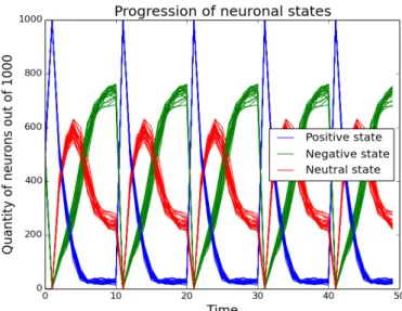
Abstract. Here we have developed a mathematical model of a random neuron network with two types of neurons: inhibitory and excitatory. Every neuron was modelled as a functional cell with three states, parallel to hyperpolarised, neutral and depolarised states in vivo. These either induce a signal or not into their postsynaptic partners. First a system including just one network was simulated numerically using the software developed in Python.

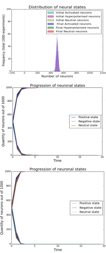
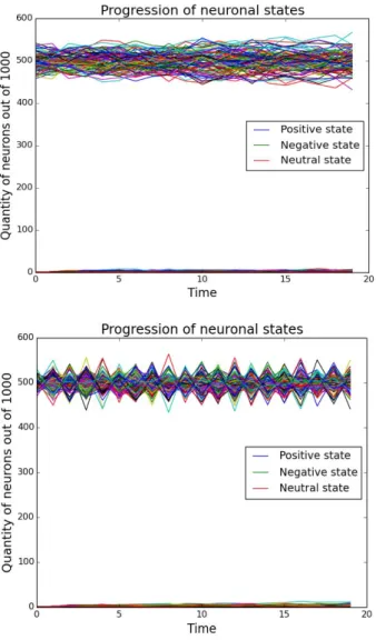
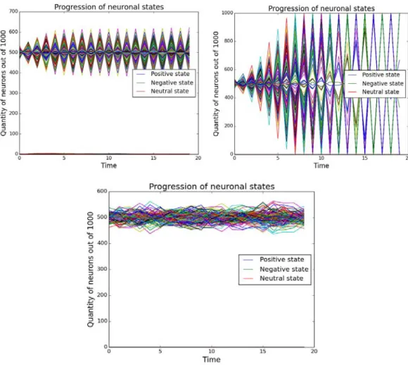
Our simulations show that under physiological initial conditions, the neurons in the network all switch off, irrespective of the initial distribution of states. However, with increased inhibitory connections beyond 85%, spontaneous oscillations arise in the system. This raises the question whether there exist pathologies where the increased amount of inhibitory connections leads to uncontrolled neural activity. There has been preliminary evidence elsewhere that this may be the case in autism and down syndrome [1-4].

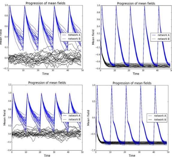
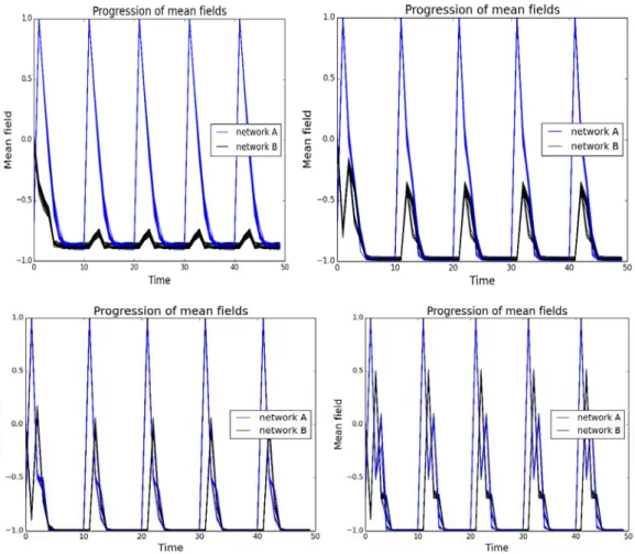
At the next stage we numerically studied two mutually coupled networks through mean field interactions. We find that via a small range of coupling constants between the networks, pulses of activity in one network are transferred to the other. However, for high enough coupling there appears a very sudden change in behaviour. This leads to both networks oscillating independent of the pulses applied. These uncontrolled oscillations may also be applied to neural pathologies, where unconnected neuronal systems in the brain may interact via their electromagnetic fields. Any mutations or diseases that increase how brain regions interact can induce this pathological activity resonance.

Our simulations provided some interesting insight into neuronal behaviour, in particular factors that lead to emergent phenomena in dynamics of neural networks. This can be tied to pathologies, such as autism, Down's syndrome, the synchronisation seen in parkinson's and the desynchronisation seen in epilepsy. The model is very general and also can be applied to describe social network and social pathologies.

Keywords: Dynamical modelling and synchronization phenomena in mutualistic neural networks, social network, social viruses.

∗

The Sainsbury Laboratory, University of Cambridge, Cambridge, UK

∗∗

School of Science, Loughborough University, UK

1. Introduction

The Ising model is a well known in physics to describe magnetic matter. It considers the spin states of each atom, which change over time with respect to the spin states of its neighbours. It is often used to analyse and predict dual opinion distributions in a model population of people. The Ising model itself is well described; however, the steps in changing the model to handle neuronal behaviour have not been tested previously. Here we systematically alter the Ising model to move it closer to a neuronal model, and look at the effect of each change. The 3 steps we look at are:

1. Randomising the neighbours.

2. Introducing a threshold.

3. Changing the polarity of the connection.

2. Methods

The Ising model we will begin with has 3 connections for each element in the network, creating a regular lattice. We sum the states of the neighbours to determine the new state of the element using the signum function. The states can be either +1 or –1. 20 time step iterations were applied, since the final state was always seen before 15t. Any changes that we applied will be described in each subsection.

The Hamiltonian of the classical Ising model is shown in equation 1:

Ising ij i j i i

H = ∑ J σ σ − ∑ H σ ⁽¹⁾

where J

is the coupling constant between spins at sites i and j. σ is the spin state, which takes the value of ±1. H is the magnetic field acting on the

spin located at site i. This model normally describes the magnetic states in condensed matter.

We now will alter the traditional Ising model, to bring it closer to neuronal style behaviour. For this we added a threshold (μ) into the signum function, as well as the state σ having 3 possible states. These states can be:

+1 for active, –1 for hyperpolarised, 0 for inactive. Therefore the state σ for neuron α can be written as follows:

1

0 0 .

1 0

if sig

sig if sig

α

+ > μ

⎧ ⎪

σ = ⎨ ≤ ≤ μ

⎪ − <

( ) (2)

Sig here is the signal received from neuron α's inputs. The signal is the sum of the weighted states of its inputs. For example the signal applied to neuron α is shown in equation 3:

1 jn

j j

j j

sig C

α

α α

= α

= ∑ σ ⁽³⁾

where C

is the coupling constant between the input j and the neuron α.

This signal then affects the new state of the neuron following equation 2.

This can be succinctly written as equation 4, by the average of 2 signum functions (for the case where all 3 states are correctly implemented):

( ) 1 [ ( ) ( )]

sig 2 Sgn sig Sgn sig

α α α

σ = + − μ (4)

These equations can be combined into equation 5, which is similar to a discretised Hopfield model.

1

( 1)

( ( ))

.

j

t Sgn C H t

α =

⎡ ⎤

σ + = ⎢ σ − μ ⎥

⎢ ⎥

⎣ ∑ ⎦ (5) Where H(x) is the Heaviside step function, and μ is the action potential threshold. The next step in progression of this model would be to correctly implement a functional hyperpolarised state. This will lead to the threshold being dependent on the prior state of a neuron (equation 6). A hyperpolarised cell is harder to activate than a cell at resting potential.

0.136 ( ) 0 ( ( ))

0.227 ( ) 0 if t

t if t

⎧⎪ σ ≥ μ σ = ⎨

σ <

⎪⎩

These values are calculated based on the resting potential of a neuron being –70mV, the threshold being –55mV, hyperpolarised potential being – 80mV and the fully depolarised state being +55mV.

For each experiment, a network of 1000 neuronal objects was built.

Each neuron is randomly assigned 3 inputs from the 1000 objects, and each

connection is given a polarity. A positive polarity reflects an excitatory

glutamatergic synapse, and a negative connection is an inhibitory

cholinergic synapse. The initial states are randomly picked from a uniform

distribution, according to a fixed ratio of ±1. The same is done with the

polarity. The inter-neuronal coupling constant is set at 0.1, and the

threshold is set at 0.136. This threshold is equivalent to a neuron reaching threshold in vivo. A zero state in our model corresponds to –70mV, threshold –55mV, and +1 state being fully depolarised at +30mV in vivo.

The states are then iterated with accordance to equations 2-4 above. This simulates the evolution of the neuronal states after we set their initial conditions. There are two possible outcomes for the system. Either the neurons reach some constant final distribution of states, or oscillations arise. A constant final arrangement is where there is no information transfer in the system, whereas oscillations indicates that there are dynamic signals at play. We predict that the final behaviour of the system can be controlled by varying the initial conditions. We will test which initial variables affect the final evolution most strongly.

Following a pilot simulation, it was seen that the system reaches a final behaviour, whether stationary or oscillatory, after 25 time step iterations. Therefore that was the maximum number of time steps we used in future runs. 50 experiments were created for each set of initial ratios, and the results collected on the same graphs to visualise clearer averages.

3. Results

1. Randomising the neighbours:

Here instead of using 3 neighbours that are fixed with respect to each

element, we used a random number generator with a uniform distribution

to select a neighbour from anywhere in the network. Here we found that

having random connections increases the magnitude of divergence in the

system. Where the original Ising model only spreads out slightly dependent

on the initial conditions, our version diverges greatly even when we

initialise with a 50:50 state split. In the symmetric case, both 1 and –1 can

win out, seen by a mean of 50 (out of 100 elements) across 100

experiments. The final states do not oscillate, tested by running 200

iterations on each experiment. Increasing the connectivity has no visible

effect on the divergence.

Figure 1. Following the states of the neurons with each iteration step from at initial 50:50 state distribution. All experiments diverge fully, seen more clearly in the histogram figure 2a.

Figure 2. a (above) A histogram with the final states of 1000 experiments.

The magenta and cyan peaks are the initial state distributions, and as we can

see the final states either all become 1 or all become –1. In contrast, figure

2b (below) shows the same results but for the original Ising model. Here the

final states have barely diverged.

2. Adding a threshold:

Adding just a threshold whilst keeping the fixed connections of the original Ising model causes an even faster full divergence (Figure 3b), where the –1 state always takes over the whole system. This makes sense, since a threshold adds in an asymmetry, and so an initial 1:1 distribution is off center from the threshold point. For the 1000 experiments, the means for the –1 state was 1000 out of 1000 elements, with a variance of 0 (Figure 3a).

Figure 3. a (above) A histogram of the state distributions. From the initial 1:1 state split, the –1 state takes over all 1000 elements, seen by the very fine lines at 1000 and 0 respective to the –1 and 1 states. The variance for both final peaks is 0. b (below) shows that the rate of divergence is a lot faster and stronger than with just the random connections (figure 1).

Adding both the threshold and random connections gives results very

similar to just the threshold Ising results, as seen in figure 4. Therefore, we

can assume the threshold effect is stronger and dominates the effect of the

random connections. However, we will still test both random and fixed

neighbours in later tests for completion.

Figure 4. The progression of states in the system with respect to time.

Initially we have a 1:1 distribution, which rapidly diverges so that the

negative states win out.

3. Adding connections with negative polarity.

We now induced a connection polarity at each input, acting multiplicatively upon the inputs to an element. Looking at the histograms, there wasn't much information seen. However, some interesting phenomena arose when looking at their progression with respect to time.

First we looked at only adding the polarity to the Ising model. Here, as the amount of negative connections increases, a phase-like phenomenon appeared, flipping the states of the system with every iteration (Figure 5).

Figure 5. a,b,c going top to bottom. 5A is the Ising model with 30%

inhibitory connections. The state frequencies remain more or less constant.

B Here the model has 70% negative connections, and an oscillatory

Now we add in having random neighbours into the model. Having 30% negative connections suppresses the divergences seen in prior runs, shown in Figure 6a. However, with 100% negative connections, divergence is seen alongside the oscillatory behaviour (Figure 6b).

Adding in the threshold so that all 3 factors are in play, we seen a return of the strong divergence of state frequencies. With 30% negative connections, the –1 state still fully wins out (Figure 7a). But as the negative connections increase up to 70%, this separation is reduced. At 100% negative connections, the oscillatory behaviour wins out again.

Figure 6a (above) and b (below): a, The progression of states of 50

experiments with random neighbours and 30% negative connections. The

negative connections seem to suppress the divergent activity seen from

Figure 1 and 2a. B, The progression of states with random neighbours, but

now with 100% negative connections. Hence the divergence is seen

partnered together with the state flipping phenomenon.

Figure 7 a,b top to bottom previous page, c above: Progression of states of 50 experiments, all with random neighbours, having a threshold and varying the amount of negative connections of 30% (a), 70% (b) and 100% (c). At 30% the –1 state wins out. At 70%, the negative connections seem to suppress this winning state. At 100%, the oscillations return that were seen in Figure 6.

Note: I have altered the code to make each population of states it's own separate colour .

With more time I'd redo these results to produce clearer graphs.

These oscillations found here occur at unphysiological amounts of

inhibitory connections, when 85% of coupling constants C are negative

(equation 5). However, this raises the question if there exists a pathology

that could increase the amount of inhibitory synapses in a particular brain

region. This would lead to any signal causing uncontrolled oscillatory

activity spike, such as those we see in simulations. There has been

evidence that increased inhibitory activity can disrupt the excitatory-

autism and down's syndrome (Baroncelli et al., 2011; Zikopoulos and Barbas 2013).

From these tests, it appears under normal physiological inhibitory ratios, any initial signal decays rapidly till the system is at rest. Therefore a good next step is to apply pulses of activity to our model network, and follow their evolution. There are 4 features that can be tested when pulses are applied to the networks: pulse rate, inhibitory ratio, intra-network coupling, and finally how pulses can be transferred via meanfield coupling to the other network. We'll start with looking at a single network.

Figure 8 a,b,c top to bottom next page. Following a network's evolution

with a pulse applied every 5 time steps. The blue network has the pulse

applied, the black network is the control without pulse. From top to bottom,

the networks have 20% (a), 15% (b) and 10%(c) inhibitory connections. The

lower the amount of inhibitory connections, the slower the activity decays in

the system. This is similar to the saturation seen in real neurons under tetanic

stimulation.

Figure 9 a,b (top): Simulations ran with increased pulse rate of every 2 time steps. A, This simulation has 20% inhibitory connections, but with pulses every 2 time steps. As you can see there is not enough time for the signal to decay fully, leading to activity similar to unfused tetanus. B, here is the same experiment as in a, but the 2 networks are allowed to interact with meanfield with strength 0.1. Here the second network seems to increase the recovery rate of neurons in network 1, almost via a dampening effect. This will be investigated later. C (below), Here the pulse rate in only every 5 time steps, with an inhibitory ratio of 15%, like in figure 8b. The difference is that the 2 networks are allowed to interact via meanfield. This leads to tetanus in both networks. This tetanus is lost when the inhibitory ratio is 20%, as in 9b, even with increased pulse rate.

Before investigating the meanfield interaction between two networks further, we will test the couping constant with in a single network first.

There are 3 possible useful coupling constants C when using 3 input

neurons, as we are using. These are when you only need 1, 2 or 3 inputs to

μ

>

C (10c), C > μ / 2 (10b), C > μ / 3 (10a). The results here are unusual however. You'd expect that when > μ / 2 > C > μ / 3 , the decay rate would be faster than for the other 2 cases. However, there are appears to be a sweet spot when C = 0.1, that leads to the fastest signal decay, similar to when C < μ / 3 (10d)

Figure 10 a-d (left to right). Simulations altering the intra-network coupling constant C. Pulses are applied every 10 time steps, inhibitory ratio in 20%.

The black lines are the control, non pulsating networks, and pulses are applied

to the blue network. The constants tested were 0.05 (a), 0.1 (b), 0.2 (c) and

(0.01, control) with a threshold of 0.136. The fastest decay rates are

observed for b and d. This results seem odd.

Figure 11 a-d (left to right). Simulations with increasing inter-network

coupling constants. Inhibitory ratio was 20%, pulses every 10 time steps into

network A (blue). The constants tested here were 0.01 (a), 0.05 (b), 0.995 (c)

and 0.100 (d). a: The coupling is too weak, so only a small reaction is seen

in network B. As the coupling constant increases through to 0.99, the

reaction signal in network B gets stronger, as well as both activation peaks

getting narrower. The narrowing seen is not intuitive, and facilitates a faster

recovery rate. Between c and d, the very small increase in coupling constant

leads to a much larger increase in Network B activity. Therefore the

coupling of 0.1 appears to be a threshold for effective cross network

signalling.

Figure 12 (above): This is a plot following the 3 state populations in the simulation from figure 11d. The positive state mirrors the meanfield seen in previous figures. The neutral “0” state appears to have a quicker reaction speed, and acts as the intermediate state moving neurons from state +1 to state –1.

Figure 13 a(left), b(right): Simulations with higher inter-network coupling.

Inhibitory ratio is 20%, pulses every 10 time steps. A: The coupling constant

here was 0.145. The reaction signal in Network B is only slightly higher than

seen in figure 11d. This further suggests that a constant of 0.1 is all that is

required for clean signalling. However, a slight increase to a coupling of

0.1475 between networks (b) shows uncontrolled resonance between both

networks, masking the pulse activity completely. This suggests another route

for pathological action.

4. Conclusions

Here we studied Ising like model applying to a broad range of system. We found some uUnderstanding the emergent phenomena in interacting neural networks that, we believe, would open up new possibilities to characterize various neural conditions. Recent research on social networks shows similar phenomena such as for example that our mood is far more strongly influenced by those around us than we tend to think. Not only that, we are also beholden to the moods of friends, or friend of friends, and of friends of friends of friends – that is, people three degrees of separation away from us. The disposition of people around us can pass through our social network like a virus and we influence each other at least on a distance of three degree of separation.

A whole range of phenomena such as happiness and depression, obesity, drinking and smoking habits, ill-health, the inclination to turn out and vote in elections, a taste for certain music or food, a preference for online privacy, even the tendency to attempt or think about suicide are transmitted through networks of friends. The ways how this Is transmitted has psychological routes and are not entirely understood. One thing is clear that the information about mood, habits and other staff we or our friends or friends of friends have propagate through the network like electricity through a power network. Although we have studied here the neuron excitations the model also shows how the social viruses are propagating through the social network and became dominant., For more detail about this aproach, see the Refs[5-12].

REFERENCES

[1] Uzunova, Genoveva, Stefano Pallanti and Eric Hollander, Excitatory/inhibitory imbalance in autism spectrum disorders: Implications for interventions and therapeutics, The World Journal of Biological Psychiatry 17.3 (2016): 174-186.

[2] Baroncelli, Laura, et al., Brain plasticity and disease: a matter of inhibition., Neural plasticity 2011 (2011).

[3] Baroncelli, Laura, Lamberto Maffei and Alessandro Sale, New perspectives in amblyopia therapy on adults: a critical role for the excitatory/inhibitory balance.

Front. Cell. Neurosci 5 (2011).

[4] Zikopoulos, Basilis and Helen Barbas, Altered neural connectivity in excitatory and inhibitory cortical circuits in autism (2013).

[5] Kusmartsev, F. V., About formation of electron strings, Journal de Physique iv, 9, 321-323 (1999).

[6] K. F. V. Kusmartsev, Formation of Electron Strings in Polar Narrow Band Semi-

F. V. Kusmartsev, D. Di Castro, Gianestra Bianconi and A. Bianconi, Transformation of Strings into Stripes and itinerant Free Carriers in HTSC, Phys. Lett. A275 118 (2000).

[7] Kusmartsev F. V., Electronic molecules in solids, EuroPhys. Lett. 54, 786-792 (2001).

[8] Kusmartsev, F., Electronic molecules in semiconductors and other novel materials, Contemporary Physics, 453, 237-250 (2004), ISSN 0010-7514.

[9] N. N. Kovaleva, K. I. Kugel, A. V. Bazhenov, T. N. Fursova, W. Lser, Y. Xu, G. Behr and F. V. Kusmartsev, Scientific Reports (NATURE) 2, 890 (2012) doi:

10.1038/srep0089.

[10] F. V. Kusmartsev, K. E. Kürten, Physics of the mind: Opinion dynamics and decision making processes based on a binary network model, International Journal of Modern Physics B (IJMPB) Vol. 22, No: 25/26, Year: 2008,

pp. 4482-4494.

[11] F. V. Kusmartsev, K. E. Kürten, Chaotic Modes in a scale free opinion networks, International Journal of Modern Physics B (IJMPB) Vol. 23, No: 20/21 Year:

2009, pp. 4001-4021.

[12] Kusmartsev, V. F. and F. V. Kusmartsev, Modelling a network where the opinion of each unit varies according to a majority ruling of its neighbouring units, arXiv preprint arXiv:1605.04596 (2016).

[13] Kusmartsev, V. F. and F. V. Kusmartsev, Modelling a network where the opinion

of each unit varies according to a majority ruling" of its neighbouring units,

Hyperion International Journal of Econophysics & New Economy 7.2 (2014).