Yes, the CAPM is testable

Yes, the CAPM is Testable

Abstract

1. Introduction

One of the central results of the Sharpe (1964), Lintner (1965) and Black

(1972) (henceforth SLB) Capital Asset Pricing Model (CAPM) is that the

relationship between beta and expected returns is linear, exact, and has

a slope equal to the expectation of the (e¢ cient) market portfolio excess

return. Despite its appeal, this prediction has found little support in more

than three decades of empirical studies. This is probably not surprising.

Empirical tests usually employ observed variables, while none of the variables

involved in empirical tests of the CAPM are directly observable.

Cross-sectional tests of the CAPM involve replacing true variables with estimates

and proxies. Expected returns are proxied by average realized returns, betas

are estimated from a sample of time series returns, and the market portfolio

is proxied by an index. Averaging realized returns and estimating betas

introduce estimation error and, hence, a¤ect the power of empirical tests.

However, they do not change the fundamental behaviour of the SLB model.

On the other hand, employing indexes other than the true market portfolio

appears to fundamentally change the behaviour of the SLB model (Roll,

1977; Roll and Ross, 1994; and Kandel and Stambaugh, 1995).

Kandel and Stambaugh (1995), henceforth KS, found that Ordinary Least

Squares (OLS) estimates of beta-return relation bear no relation to the

prox-imity of an ine¢ cient index to the e¢ cient frontier. More importantly, KS

show that while OLS estimates are of little use, Generalised Least Squares

(GLS) estimates are functions of known quantities that are exactly related

to the position of the index within the mean-variance frontier. These can be

used to assess how close the used index is to the e¢ cient frontier. But while

the GLS quantities derived in KS are useful for testing the e¢ ciency of a

this paper is to extend the results of KS and show that, if the CAPM is the

true generating process, these GLS quantities can be used to test it.

KS investigated the e¤ect of using an ine¢ cient proxy on the CAPM

un-der the assumption that some version of the CAPM holds. This assumption

may not be correct, as expected returns may well be described by, say, some

unknown multifactor model. In such a case, the KS results no longer hold

because we now have an additional source of misspeci…cation, namely the

omission of some relevant risk factor(s). The second aim of this paper is to

show that there is a simple way to test the CAPM even when the

assump-tion that the CAPM is the true generating process is incorrect. I achieve this

by using the coe¢ cient of determination from both OLS and GLS methods,

which can help distinguish cases of ine¢ cient indexes from cases of omitted

unobserved variables.

This paper is closely related to Grauer and Janmaat (2009) and

Murtaza-shvili and Vozlyublennaia (2012). These authors provide useful simulation

results and brie‡y review the literature related to what Grauer and Janmaat

(2009) call the …rst stream of literature, which is mainly concerned with the

power of empirical tests of the CAPM. However, while the present paper has

empirical implications, it falls within what Grauer and Janmaat (2009) call

the second stream, which focuses on population parameters and the

funda-mental economic behaviour of the CAPM.

The rest of the paper begins with a summary of the full procedure

pro-posed in this paper in Section 2. In Section 3 the true cross-sectional relation

between expected returns and beta computed from any index is outlined.

Sec-tion 4 removes potential ambiguity by giving a clear idea of what is meant

by a ‘correctly speci…ed’ or ‘true’ model. In Section 5 I show how we can

a direct test of the CAPM under the assumption that the CAPM is the true

generating process. Section 6 deals with potential non-CAPM models, and

proposes a simple procedure to simultaneously assess the e¢ ciency of the

index and the presence of omitted factors. Section 7 provides a simulation

experiment to demonstrate the behaviour of the OLS and GLS statistics.

The …nal section concludes.

2. Summary of the Proposed Test

In this paper I will employ the following notation, which is similar to the

one used in Roll and Ross (1994), henceforth RR,1

R is the expected returns vector for N individual assets,

V is the N N covariance matrix of returns,

1 is the unit vector,

Bold lower case letters (i,m, qand p) are portfolio weights vectors,

i = ( 1i 2i N i)0 =Vi= 2i,

ri =i0R is the expected return of portfolio i,

2

i =i0Viis the variance of portfolio i.

The testing procedure I propose is simple. It is based on the idea that

both OLS and GLS R2 _{will only attain the maximum value of one if there}

were no omitted factors and the index used to compute beta is e¢ cient.

A general true process generating expected returns can be written as

R=rzm1+ p p+ ep+d

where rzm is the true market portfolio’s zero beta rate, p is a parameter,

and the vector _p is computed against a possibly ine¢ cient portfoliop. Even

1_{Like RR and KS, I assume that expected returns and the covariance matrix of these}

without measurement errors, cross-sectional tests of the CAPM have to

con-tend with two unobserved error terms. Both terms are generally correlated

with the regressor ( _p) and hence lead to systematic biases. The …rst error

term, ep, is due to possible ine¢ ciency of the index used to compute p.

The second term, d, is due to the possibility that the CAPM is not the true generating process.

If expected returns are explained by an e¢ cient portfolio beta, then

d =0. We can only ensure that d=0 if both OLS and GLS R2 _attain

their maximum value. The …rst step, therefore, in testing the CAPM would

involve testing the null

H01 :R2gls =R

2

ols = 1:

If this hypothesis is accepted, this would con…rm that some form of beta

model holds and that the index used in computing beta is e¢ cient. The next

step consists of testing the hypothesis that the sum of GLS-estimated slope,

p(gls), and intercept, rzp(gls), are equal to the expected index return, rp.

In other words, the second step tests the following null

H02 :rzp(gls) + p(gls) rp = 0

Failing to reject this second hypothesis would con…rm that the index is

indeed the market portfolio and that, consequently, the CAPM holds.

3. Ine¢ cient Indexes and the True Relation between Expected Re-turns and Beta

In this section I o¤er a simple representation of the relation between beta

holds, there exists an e¢ cient market portfolio,m, for which expected returns have the following exact linear relation

R=rzm1+ m m (1)

where rzm is portfolio m’s zero beta rate, and m = rm rzm is the risk

premium. The vector _m = ( _{1m 2m N m})0 _{is computed against the}

e¢ cient market portfolio m. If we were to observe m, model (1) can be

used to …nd the exact zero beta rate and the risk premium. However, given

V, observing m is dependent upon observing the e¢ cient portfolio m. In

practice, though, it is almost impossible to observem. Suppose that instead we use an observable, but possibly ine¢ cient, index p. Two questions arise: (i) what would the true relation between beta computed on the observed

index and expected returns be; and (ii) can we still test the CAPM given

that we are using possibly the wrong index? The answer to the last question

is yes. This is achieved by …rst …nding out whether or not we are using an

e¢ cient index and then proceeding to assess whether the e¢ cient index is

the market portfolio. This is discussed in subsequent sections. Before that,

I will attempt to answer the …rst question.

We can write the possibly ine¢ cient portfoliop as a deviation from the e¢ cient market portfolio, that is

m=p+Dp (2)

Replacing in (1) gives

R = rzm1+ m₂ m

Vm

= rzm1+ m

2

m

Vp+ m 2

m VDp

= rzm1+ _{p p}+ep (3)

where p = m 2p= 2m and ep = ( m= 2m)VDp is the (unobserved) pricing

error vector. This result is identical to that of Ashton and Tippett (1998,

p.1333) except that they write ep in terms of N 2 arbitrage portfolios.

Clearly, the relation between _p and R is less than perfect because of the presence of the pricing error ep.

The inability to observe the e¢ cient market portfolio, m, and the use of an ine¢ cient proxy, p, is equivalent to assessing the relation between p

and R. Thus, when the CAPM holds, the true model governing the relation between mandRis (1), while the true model governing the relation between

p and R is (3). Both (1) and (3) are true models, but the reason why we

are interested in (3) is our utilization of the ine¢ cient index p.

An objection might be that there exists an in…nite number of

‘true’mod-els,

R=rzm1+ p p+ep; (4)

where _p and e_p are appropriately chosen. For example, _p = _{p p} and

e_p = ep + (1 ) p p, for any arbitrary , are all deviations from (3).

However, this is trivial since they all simplify algebraically to (3), which is

the unique true relation between p and R.

The point that any arbitrary model (4) reduces to (3) seems to have been

missed by KS. These authors assume that expected returns are given by

error vector. This model is identical to (4) with = [rzm p]0 and X = [1

p]. The true parameter relating p toR is p and not an arbitrary p (or,

alternatively, ).

A question that arises is whether there can be models where the true

parameter relating _p toR is di¤erent from _p. In other words, is it possible to have a model like (4) that reduces to (1) without passing through (3)?

The answer is yes, but such a model would be inadmissible in a world of

CAPM as it would imply that the index used in the test is not fully funded.

One interesting example is the deviation suggested by Ferguson and

Shock-ley (2003), who assume that the true market portfolio consists of a weighted

sum of the economy’s debt claims (D) and the economy’s equity claims (p)

m= p+ (1 )D

where 0< <1.

In our notation, pis an (observed) ine¢ cient index andD is the omitted portfolio with D0_{1= 1. Replacing the value ofm in equation (1) yields}

R=rzm1+ p p +

(1 ) 2_{D m}

2

m

D (5)

Thus, the implicit assumption in this model is that the index used in

computing betas is not fully funded ( p rather thanp) and this violates the budget constraint in the CAPM optimization problem.

A simple conclusion from model (3) is that the true cross-sectional slope

( _p) between expected returns and beta computed against any portfolio is

always positive. However, although the true slope is non-zero, the empirical

estimate of _p may not be so. Assuming we can measure _p precisely,

esti-mating rzm and p in model (3) su¤ers from the omitted regressor problem

Whenpis on the upper half of the e¢ cient frontier,epwill be uncorrelated with p but correlated with the vector 1. Thus, the GLS/OLS estimators

of rzm are still biased, but they will both produce a perfect …t (as we shall

see later). The reason is that betas computed from e¢ cient portfolios are

perfectly correlated.2 _{So although the estimators are biased with respect}

to the true model (1), any beta computed against an e¢ cient portfolio has

a perfect linear relation with the cross-section of expected returns. I will

exploit this divergence to derive a criterion for testing the CAPM.

Whenpis not on the e¢ cient frontier, the empirical power of _p to explain expected returns may or may not depend on the position ofp relative to the e¢ cient frontier. A signi…cant …nding by KS is that the choice of OLS versus

GLS is critical. Although both methods yield biased estimates with respect

to the true model, under OLS the empirical power of _p suggested by the

estimates (including the R2_{) bears no relation to the proximity of portfolio}

p to the e¢ cient frontier. The bias can be arbitrarily large or small.

On the other hand, under GLS the power of p to explain expected

returns is strictly related to the position of portfolioprelative to the e¢ cient frontier. The bias in both parameters is known exactly. Hence, one can use

this GLS feature to assess the position of the proxy not only with respect to

the e¢ cient frontier but also with respect to the true market portfolio.

It is worth noting, however, that while KS have successfully explained the

bias of the GLS estimator, they do not seem to have explained the behaviour

of the OLS bias satisfactorily. Appendix 1 revisits KS analysis, with a view

to providing a better explanation of the OLS bias.

4. Terminology: “Correctly Speci…ed” and “True” Model

2_{If bothmandpare e¢ cient,}

p and mwill be perfectly correlated because they are

Before discussing the proposed tests it is useful to remove potential

am-biguity that can arise from the use of the terms ‘correctly speci…ed model’

and ‘true model’. The latter is related to the real world, so when we say

that the CAPM is true (or, alternatively, that the CAPM holds), we simply

mean that the data are actually generated by a CAPM model. The former is

related to the empirical world. So when we say that the (empirical) model is

correctly speci…ed, we simply mean that the empirical model’s speci…cation

coincides with the real data generating process.

In our context, a true expected return generating process can be written

in the following general form R=rzm1+ m m+d. This model allows for

any cross sectional speci…cation, such as APT or other multifactor models,

through the vector d. When d=0 I say that the CAPM holds, or the CAPM is true. This simply means that the assumption that ‘the CAPM is

the process that has generated the observed expected returns’is correct. An

empirical CAPM model of the form R = rzm1+ _{m m} +", where " is the usual disturbance term,3 _{will be said to be correctly speci…ed. But this only}

happens when we observe the market portfolio (i.e. when we use m as a

regressor).

Incorrect speci…cation, or misspeci…cation, takes place for two reasons.

Either we wrongly assume that the observed portfolio is the market portfolio

(ep ₆= 0); and/or we wrongly assume that the CAPM holds (d₆= 0). Thus, the (possibly non-CAPM) true model will be R = rzm1+ p p+ep +d,

whereas the empirical model will beR=rzm1+ _{p p}+", but the disturbance term will no longer have zero mean or be uncorrelated with the regressor p

(since "=ep+d).

3_{This term is usually assumed to have zero mean and to be uncorrelated with}

regres-sor(s). In this paper I assume away statistical or measurement errors, so in this case of

Any inference carried out on the CAPM therefore crucially depends on

whether the assumptions that the ‘CAPM is true’ and that ‘the portfolio

used to compute beta is the true market portfolio’ are correct. If both

as-sumptions are correct, then we would only have to contend with small sample

or measurement errors (which are assumed away in this paper). However,

when one or both of these assumptions are incorrect, then we would have to

contend with the meaningfulness of the empirical estimation and inference.

In the next section, I will show that the CAPM can be tested in the

simpler case where the assumption that the CAPM holds is correct (d=0), but the only potential problem is the possibility that the index is not the

market portfolio (ep ₆=0). However, the inference will generally be invalid if the CAPM assumption is violated. Fortunately, there is a way to ensuring

that d=0 before proceeding with the formal test of the CAPM. This is discussed in Section 6.

5. Testing the CAPM under the Assumption that the CAPM Holds

In this section I extend the results of KS, who show that the GLS method

provides a useful statistic, namely the GLS R2_{, that can be used to assess}

the e¢ ciency of a given portfolio. I emphasise the point that KS build their

results under the assumption that the CAPM is true. I will use the same

assumption in this section to (i) show that the e¢ ciency of a portfolio is a

necessary but not su¢ cient condition for testing the CAPM; and (ii) derive

a necessary and su¢ cient condition for testing the CAPM.

I start by showing the usefulness of GLS. The GLS bias, derived by KS

(p.167), is given by

0

@ ^rzm(gls)

^_m(gls) 1 A=

0 @ rzm

m

1

A+ 1 _p 0 @ m

2

g

2

m

m

where _p = (rp rg)=(rm rg), and rg is the expected return of the Global

Minimum Variance Portfolio (GMVP). For ine¢ cient portfolios above the

GMVP (rp > rg), the intercept is always overestimated and the slope is

al-ways underestimated. Also, for rp > rg, both GLS estimates will be positive.

The slope bias is completely determined by portfolio p’s position in mean-variance space, but the intercept bias is only partially determined by p.

Thus, for a given portfolio, di¤erent asset universes will produce identical

slope biases but di¤erent intercept biases.

As KS argue, the OLS estimator o¤ers no clues as to where portfolio p

is situated relative to the e¢ cient frontier. Relying on OLS can therefore

be misleading. On the other hand, the GLS result is strictly related to the

position of the ine¢ cient portfolio in mean-variance space. The question

then is how useful is GLS in testing the CAPM? The answer is that the raw

quantities obtained from GLS are only useful for testing the e¢ ciency of a

given index. To see this, note that in the absence of sampling error, the GLS

output contains three quantities: the intercept, rzm+ (1 p)(rg rzm), the

slope p(rm rzm), and the GLSR2 given by4

2

p =Rgls2 = 1

(R X gls)0V 1(R X gls) (R 1 )0V 1_{(R 1 )}

where = (R0V 11)=(10V 11).

All three quantities depend on the measure of the relative e¢ ciency of

portfoliop, p. Although the intercept is uninformative, the sign of the GLS

slope tells us the position of the index relative to the GMVP. A positive

value of the slope indicates that the index is above the GMVP and vice

versa. The R2

gls informs us how close the index is to the frontier. Thus, only

by combining the information contained in the slope and the R2_gls can we determine the exact position of the ine¢ cient index.

4_{The proof that} 2

However, determining the e¢ ciency of a given index is not su¢ cient for

testing the CAPM. Suppose the slope was positive and 2_p = 1. This would only tell us that portfolio p is e¢ cient, but this would not be su¢ cient evidence in favour of the CAPM. In other words, the e¢ ciency of an index

is a necessary but insu¢ cient condition for the CAPM to hold.

Although any e¢ cient portfolio will provide perfect linearity and hence

perfect …t, the CAPM requires that the slope equals the market expected

return in excess of the zero beta rate, and that the intercept equals the zero

beta rate. However, if an index, say q, is e¢ cient the GLS regression would give two positive numbers

q gls =

0

@ r^zq(gls)

^_q(gls) 1 A=

0 @ rzq

rq rzq

1 A

If the index is the market portfolio we would also be given two positive

numbers

m gls =

0

@ ^rzm(gls)

^_m(gls) 1 A=

0

@ rzm rm rzm

1 A

Both q and m will satisfy 2_m = 2_q = 1. Telling the di¤erence between

q and m is the key to the testability of the CAPM. Using the relationship betwen the GMVP and any e¢ cient portfolio, we have

rg =rzq+ (rq rzq)

2

g

2

q

rg =rzm+ (rm rzm)

2

g

2

m

Combining these two equations gives

rq =rzq +

2

q

2

g

(rzm rzq) +

2

q

2

m

From (3)

R = rzm1+

2 q m 2 m q+ m 2 m

(Vm Vq)

= (rzm+ q m₂ m

)1+ 2

q m

2

m q

= rzq1+(rq rzq) _q (7)

where q is a constant and results from the fact that q and m are perfectly

correlated. Suppose we estimate a model using the e¢ cient portfolioq. Using (7) we have

^

rzq(gls) + ^q(gls) = rzq+

2

q

2

m(rm rzm)

Subtracting (6) from above yields

^

rzq(gls) + ^q(gls) rq =

2

q

2

g(rzm rzq)

which only equals zero if q=m.

Thus, GLS can help us not only to determine the e¢ ciency of a given

index, but also to test the CAPM. It exploits the fact that under the null

(q=m)

^

rzq(gls) + ^q(gls) rq = 0

So, one can test whether the sum of slope and intercept are equal to the

expected index return. Note that when the index is e¢ cient, OLS and GLS

are identical in the absence of sampling error. Thus, in principle, both

meth-ods could be useful in testing the CAPM. However, empirical investigators

use sample estimates of returns, betas and the covariance matrix. That is,

empiricists use feasible GLS rather than GLS. So, as Shanken (1992) and

samples”(KS, p.170). Nevertheless, in practice the choice between OLS and

GLS will depend on considerations other than the population moments.

Al-though it is beyond the scope of this paper to discuss these practical choices,

it should be noted that most econometric textbooks describe to some length

the conditions under which some estimators might be preferable to others.

6. Omitted Factors

The previous analysis was based on the assumption that the SLB CAPM

holds. The only source of potential problems considered so far has been the

use of an ine¢ cient index. This follows the tradition of RR, KS and Ferguson

and Shockley (2003) who do not consider the case where the CAPM does not

hold. However, since my results support the testability of the CAPM when

it is true, I need to assess whether the CAPM can also be rejected when it

is false.

Appendix 2 shows that there is no loss of generality if we focused on

vertical departures from the market portfolio. Thus, let X = [1 _p] and

= [rzm m]0, and consider the general (possibly non-CAPM) model

R=X +ep+d

where d is not proportional to the vector1, and ep 6= d.5 This is the case

of both omitting relevant factors and using a possibly ine¢ cient index to

compute betas. When d₆=0; the previous results on GLS bias no longer hold, even if ep = 0.6 Thus, we are now faced with two potential sources

of bias, and we cannot identify whether the source of bias is due to the

ine¢ ciency of the index or due to misspeci…cation.

The bias for the OLS and GLS estimators is given by, respectively

5_e

p+d=0implies that the CAPM holds and thatpis e¢ cient.

6_{However, whendis orthogonal toXthe OLS will be unbiased, and whendis}

ols = + (X0X) 1X0(ep+d) gls = + (X0V 1X) 1X0V 1(ep +d)

It is clear that the bias would only vanish whenep =0(that is, the index used to compute beta is the market portfolio) and d is orthogonal toX (for the OLS case), or V 1X (for the GLS case). Note that the bias will remain if the index was e¢ cient but not equal to the market portfolio (that is, if ep

was proportional to the vector 1). Thus, omitting factor sensitivities may worsen the spuriousness problem because there are now two sources of bias.

More importantly, the GLS bias is no longer related to the position of the

index relative to the e¢ cient frontier. This is simply because d may not be related to V 1 and X in the same way as ep.

As a result, R2

gls loses its strict relation with the index position relative

to the e¢ cient frontier and, like R2_ols, may behave erratically. But this is not the only consequence of admitting potential misspeci…cation. In KS, and

under the assumption that the CAPM is true generating process, R2_ols = 1

or R2

gls = 1 can only happen when the index is e¢ cient. A surprising result

here is that the R2 can attain its maximal value even when the index is ine¢ cient. This is because there are now two sources of bias, ep and d,

which can combine to give R2 = 1.

To see this, note that from the de…nition of the R2

ols (Appendix 1) and R2_gls, the vectors of interest are, respectively

Qols=R X ols = [I X(X0X) 1X0] (ep+d) Qgls =R X gls = [I X(X0V 1X) 1X0V 1] (ep+d)

These are the pricing errors obtained from the OLS and GLS estimation,

respectively. Because bothR2involve quadratic terms,R2_ols= 1andR2_gls = 1

when (i) ep=0, or ep is proportional to the vector1, and (ii)d =0, that is, the index used to compute beta is e¢ cient and there are no omitted factor

sensitivities (i.e. the CAPM is true).

However, there is a possibility thatR2 _{= 1even when the above conditions}

are not met. For the OLS, when d is orthogonal to X (i.e. X0d = 0) the pricing error vector simpli…es to

Qols = I X(X0X) 1X0 ep+d

Thus, d= [X(X0_X) 1_X0 _I]e

p implies Qols =0.7

Similarly, when d is orthogonal to XV 1 (i.e. X0_V 1_{d = 0) the pricing}

error vector simpli…es to

Qgls = I X(X0V 1X) 1X0V 1 ep+d

So, d= [X(X0V 1X) 1X0V 1 I]ep implies Qgls = 0.

Thus, one could unawarily use both an ine¢ cient index while omitting

relevant variables from the empirical model and still obtain a perfect OLS or

GLS …t. Fortunately, we cannot obtain a perfect …t for both, for even in the

unlikely event thatdwas orthogonal to both matrices (i.e. X0d=X0V 1d=

0) it would not be able to satisfy Qols =Qgls = 0. The reason is that8

X(X0X) 1X0 ₆=X(X0V 1X) 1X0V 1

Thus, when the CAPM is not the true generating process (d₆=0), using an e¢ cient index actually ensures that both OLS and GLS R2 _{will be less}

7_{We exclude the case where e}

p is a linear combination of the columns of X, because

that would implyd= 0. This also applies to the GLS case below.

8_{Except for the trivial case where the covariance matrix is proportional to the identity}

than 1, regardless of whether or not d is orthogonal to X or XV 1. This highlights the danger of carrying out inference under the assumption that the

CAPM holds. Were we to do that in the presence of an omitted sensitivity,

we could conclude, wrongly, that the index is ine¢ cient on the basis of the

GLSR2_{as suggested by KS. Unexpectedly, when the index is ine¢ cient there}

is a possibility that one of theR2 _{will equal 1. Again, were we to believe one}

of theR2 _{we would wrongly conclude that the index is e¢ cient, when in fact}

it is not. Fortunately, there is a unique case where we can ensure that the

index is e¢ cient and that the CAPM is the true model, namely when both

OLS and GLS R2 _{attain the maximum value of 1.}9

Thus, one major conclusion emerges: the CAPM is testable even under

potential misspeci…cation (ine¢ cient index and omitted factor loadings). It

is well known that omitted variables create inference problems because we

do not know whether the estimates are biased or not. Econometricians are

aware of this problem and generally tolerate it, especially when the

omit-ted regressor is orthogonal to, or at least uncorrelaomit-ted with, the right hand

side variables. Most empirical models in economics accept the less than

per-fect relation between regressor(s) and regressee, and often focus on obtaining

unbiased estimates. One further advantage with economic models is that

regressors are observed (or assumed to be observed). Thus, an R2 _{that is}

smaller than 1 is not a cause for concern. In CAPM language, this is

equiva-lent to saying that (i) the CAPM holds; (ii) the CAPM predicts an imperfect

relation between beta and expected returns; and (iii) the market portfolio is

observable. Were we to have these facilities, we would then only be interested

in the market risk premium, hoping that omitted factors sensitivities were

9_{Note that, here, e¢ cient means that the portfolio is on the minimum variance frontier.}

uncorrelated with the market beta. The R2 _{would be of no consequence.}

Unfortunately, when testing the CAPM the econometrician does not

ben-e…t from such facilities. Even with no measurement errors, the

econometri-cian still needs to show that the observed index is e¢ cient, that it is the

market portfolio, and that there are no omitted factor sensitivities (i.e. the

CAPM holds). RR argue that the …rst requirement cannot be attained using

OLS even if we assumed that the CAPM holds. KS show that index e¢

-ciency can be assessed via GLS when the CAPM holds, but do not explore

the property of GLS in a non-CAPM world. Understandably, given the

pes-simism against the testability of the CAPM, assessing whether the index is

the market portfolio and whether there are no omitted variables has not been

dealt with previously. In this paper, I o¤er a positive answer to the sceptics:

the CAPM is testable. Of course, like RR and KS I do assume measurement

errors away. What happens when there are measurement errors is a di¤erent,

and certainly more challenging, undertaking. The aim of this paper is much

more modest. I have simply attempted to establish a theoretical principle,

namely the CAPM is testable.

7. A Simulation Experiment

Although we know the exact behaviour of the GLS slope, we are far less

informed about the OLS coe¢ cients. All we know is that they are biased

and that the bias is arbitrary and is not related to the proximity of the index

to the e¢ cient frontier. Since it is not possible to assess the scale and sign of

the OLS bias theoretically, it should be useful to infer the behaviour of the

OLS estimates via a simulation experiment.

The simulation is carried out in two main steps. The …rst step involves

mean-variance universe and randomly generate deviations from the market

return, and calculate the OLS and GLS estimates of parameters and R2_.

First, to generate a mean-variance frontier, a positive de…nite

variance-covariance matrix, V, is randomly drawn such that the GMVP’s standard deviation lies between 2% and 6%. GivenV, I randomly draw a set of market weights, m, such that the market portfolio’s standard deviation is less than 30%. More speci…cally, I …rst obtain beta, _m = Vm=m0Vm, and then obtain a set of compatible expected returns, R= 1+ 2 m. The zero beta

rate 1 is drawn from a uniform distribution with a range of 0.4% to 0.6%.

The excess market return 2 is drawn from a uniform distribution with a

range of 0.65% to 0.85%: The market return and variance are then obtained as rm =m0R, and 2m =m0Vm. I redrawmand repeat the procedure until

m is less than 30%.10

Next I generate random deviations from the market portfolio to obtain

an ine¢ cient portfolio p. Since it is di¢ cult to obtain vertical deviations fromm, I generate the e¢ cient portfolio,q, that has the same variance asp. The comparison is then made between p and q. Thus, for each replication the true model is R = rzq + q q, where q = rq rzq. The OLS and

GLS estimates are obtained using p instead of q. The coe¢ cients are

then compared with the true values rzq and q. I also calculate p and the

coe¢ cients of determination for each replication.

To minimise the chance that the results are driven by an arbitrary choice

of the e¢ cient frontier, I maximise the number of asset universes used in

10_{To give an idea about the kind of frontiers I use in this simulation, I generated 5000}

the simulation. I generate 1000 di¤erent frontiers, and for each of these I

generate 1000 deviations from the market portfolio. These deviations are

computed such that a wide range of portfolio ine¢ ciency is produced. This

gives 1 million replications, producing GLS and OLS biases.

A. Comparing the Slopes.

The basis for comparing the slopes is the relative bias, which is given

by ^q q

q . However, to get an idea about how distant the estimate is from

the true value I use a slight modi…cation, 1 + ^q q

q . This shows the bias

as a proportion of the true slope. For example, a value of 0.40 means that

^_q = 0:4 _q, that is, the OLS coe¢ cient underestimates the true parameter by 60%.

The GLS and OLS biases will behave according to, respectively,

1 + ^q(gls) q

q = p

1 + ^q(ols) q

q =

cov^ ( p; q)

v^ar( p)

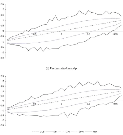
Figure 1 shows these biases for two cases, each of which depends on

whether or not a constraint of positive portfolio weights is imposed. These

are (a) constrainedmandp, and (b) unconstrainedmandp.11 _{This ensures}

that the results are not driven by short positions (RR, 1994; Grauer, 1999).

As expected, the GLS bias is exact in _p. The constrained and

uncon-strained cases are very similar and con…rm the arbitrariness of the OLS bias.

The spread around the true slope is large even for highly e¢ cient indexes.

Zero estimated slopes are not expected to be uncommon, and for indexes

that are roughly less than 80% e¢ cient we should even expect negative OLS

slopes. Yet, large estimates cannot be ruled out.

11_{The cases where only one of the two portfolios is constrained were very similar}

B. Comparing the Intercepts.

The GLS intercept has an exact relation with p, but is not exclusively

determined by it. However, it is possible to derive a bias criterion such that

it is exactly linear in p. Using the GLS bias result, and equation (A66),

p.180 of KS, I obtain

^

rzq(gls) rzq

rg rzq = 1 p

Unfortunately, this cannot be compared with a similar OLS criterion.

Using the OLS bias result gives

^

rzq(ols) rzq

rg rzq =

rq rzq

rg rzq q p

cov^ ( p; q)

v^ar( p)

So, although the GLS intercept will not depend on the frontier, the OLS

criterion will depend on three frontier parameters. The OLS bias would

appear to be arbitrary by construction. However, the above OLS criterion

simpli…es to a relative measure that will not depend on the frontier

^

rzq(ols) rzq

rq rzq = q p

cov^ ( p; q)

v^ar( p)

This gives a bias relative to the e¢ cient index return rather than the

GMVP return. The OLS and GLS bias criteria are therefore not directly

comparable. Nervertheless, there is a clear di¤erence. The weighted GLS

bias should be exactly linear with the e¢ ciency of the index. On the other

hand, the weighted OLS bias is expected to be unrelated to the e¢ ciency of

the index.

Figure 2(a) plots the relative OLS bias for the constrained case (positive

m and p). For highly ine¢ cient indexes, the OLS method seems to always overestimate the intercept. However, for more e¢ cient indexes the bias can

^

rzq(ols), cannot be ruled out. In the above experiment, around 600 intercepts

(out of the million replications) were negative.

Figure 2(b) shows a plot of the OLS relative bias when the market and

ine¢ cient portfolios are allowed to have short positions. The relation between

relative e¢ ciency and intercept seems ‡atter than that of the constrained

case, but the bias is still arbitrary.

In both constrained and unconstrained cases there is an obvious tendency

for the OLS to over-estimate the intercept. The 1st and 99th percentiles

suggest that the vast majority of cases have positive bias. As expected, the

GLS relative bias is exactly linear and is therefore not reported. Clearly, the

GLS estimate of the intercept is always biased upwards and hence always

positive.

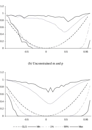
C. The R-Squared.

The R2 _{results for the experiment are plotted in Figure 3. Both}

con-strained (positive m and p) and unconstrained cases are shown. The GLS shows the expected exact curve, but the OLS bias appears to depend on the

constraint. While the unconstrained bias is smoother and fairly symmetric,

the constrained percentiles are tilted to the right. However, both cases give

the same message. The OLS varies widely with relative portfolio e¢ ciency,

p. If we take the extremes, zero R2ols are very common and can be found

for indexes that are more than 95% e¢ cient in the constrained case. Large

values for the R2

ols are also common at all levels of ine¢ ciency. In general

it is clear that the OLS does not provide guidance as to the e¢ ciency of a

given portfolio.

D. Nearly E¢ cient Portfolios.

As mentioned earlier, one advantage of the bias derived in this paper is

the bias formulas we expect the slope bias and R2

ols to converge to zero and

one respectively, as the index gets arbitrarily close to the upper half of the

e¢ cient frontier. This is shown in Figure 4, where the OLS slope bias and

R2

ols for the 4000 most e¢ cient simulated portfolios are plotted. The slope

bias is still substantial for portfolios that are 99.3% e¢ cient. However, we

can also see that the OLS slope estimates get closer to the true slope as

the portfolio e¢ ciency gets arbitrarily close to 100%, but we would not be

comfortable with portfolios that are less than 99.99% e¢ cient. For example,

a 99.8% e¢ cient portfolio can produce a slope that is anywhere between less

than 90% and almost 110% the true slope.12 _{This clearly casts doubt on the}

usefulness of OLS even with nearly e¢ cient indexes. TheR2_olsshows a similar pattern. Figure 4 shows that R2

ols of less than 0.96 can still be obtained for

indexes that are between 99.7% and 99.8% e¢ cient. Again, for very nearly

e¢ cient portfolios, the R2

ols is very close to its maximum value.

[Insert Figures 1-4 around here]

E. Omitted Factors.

The above simulations are based on the assumption that the true data

generating process is the CAPM (d=0). The R2

gls is exactly related to the

e¢ ciency of the index as expected, while the R2

ols seems to converge to its

maximum value as the index gets arbitrarily close to the e¢ cient frontier.

With potential omitted factors, the interest lies in the behaviour of both

coe¢ cients of determination. To show this, expected returns are generated

as before, except that one additional term is added to the CAPM, R =

rzq + q q+d. I generate omitted sensitivities, d = d , by taking seven

12_{These values are true for this particular experiment. Di¤erent simulations may}

di¤erent values for the scale, , starting at zero (CAPM) and then increasing

to 0.001, 0.01, 0.05, 0.1, 0.5 and 1. For each value of a random vectord is drawn from a uniform distribution with a range of 0% to 1%, and then the

whole simulation procedure is repeated (that is, 1000 di¤erent frontiers by

1000 deviations from the market portfolio). This gives one million replication

for each of the seven scales, .

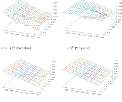
The results are shown in Figure 5. The …rst pair of plots show the 1st and

99th percentiles for theR2

ols for each of the seven scales of omission. Because

OLS is highly sensitive to repackaging, the …rst percentile is as low as 29.3%

for indexes that are 90% e¢ cient. The addition of omitted variable has some

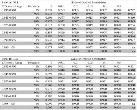
e¤ect, especially for indexes below 96% e¢ ciency. Table 1 shows the values

of the R2

ols percentiles. In general theR2ols tends to decrease with increasing

importance of omitted sensitivities. More importantly, the R_ols2 can reach the maximum value even for indexes that are not perfectly e¢ cient. This is

shown under = 0:05where the 99th percentile equals exactly 1 for indexes whose e¢ ciency is between 99% and 99.5%. Although the general trend is

for the R_ols2 to increase with increasing index e¢ ciency, the 1st percentile remains relatively low (between 97.2% and 97.9%). We also get a glimpse on

the e¤ect of more important omission at the highest scales ( = 0:5and 1). All 99th percentiles decrease relative to other lower scales. Unfortunately, I

have been unable to obtain highly e¢ cient indexes with higher scales and I

leave this intersting behaviour for a future investigation.

The GLS statistics are far less sensitive to repackaging, and show a much

smoother relation with the index e¢ ciency and the omission scale. Table

1 reveals that the di¤erence between the 1st and 99th percentiles is around

1% for all cases. The increase in the …rst …ve scale values does not seem to

be shown at the third decimal place). However, the two highest scales have

a clear impact on the 1st and 99th percentiles for the two highest levels of

e¢ ciency. For up to 99.5% index e¢ ciency, the 99th percentile goes down

from 98.9% to 98.4% when the omission scale increases from 0.5 to 1.

Sim-ilarly, when the omission scale increases from 0.1 to 0.5, the 99th percentile

decreases from 99.9% to 99.4% for the highest e¢ ciency indexes. As before,

the increase in index e¢ ciency increases the R2

gls overall.

To sum up, the impact of omitted sensitivities on the coe¢ cients of

de-termination depends on how important these sensitivities are to expected

returns. For low importance, the GLS is generally insensitive and will

de-pend mainly on the e¢ ciency of the index. The OLS is highly sensitive

and can help reject the CAPM even for very highly e¢ cient indexes. As

these omissions become more and more important, the limited results of the

simulation indicate that both R2

ols and R2gls will start to decrease sharply.

[Insert Figure 5 around here]

[Insert Table 1 around here]

8. Conclusions

Testing the CAPM has long been problematic. The use of an ine¢ cient

index is by no means its only limitation, but the possibility that the indexes

used typically in empirical tests of the CAPM are ine¢ cient undermines even

the question of whether we are really testing the CAPM or a model other

than the CAPM. The most challenging question to previous empirical studies

of cross-sectional tests of the CAPM has been whether the CAPM is testable

at all. Even assuming estimation problems away, one is still faced with two

major uncertainties: the ine¢ ciency of the market index and the possibility

In this paper I propose a new way of testing the CAPM, even in the

presence of orthogonal omitted factor sensitivities. I show that the CAPM

is testable both when the CAPM holds and when it does not. The trick

is to use both OLS and GLS. The only way that both R2 _{can attain their}

maximum value is when we use an e¢ cient index and there are no omitted

variables. Once it is ascertained that the CAPM is true and that the index is

e¢ cient, one can then proceed to formally test the CAPM using an extension

of KS results.

The results of this paper are based on the assumption that there are no

sampling errors. This assumption helps to isolate the fundamental behaviour

of the model at hand. In practice, though, the OLS and GLS estimates will

be subject to additional uncertainty due to measurement errors in expected

returns and betas. The literature has come up with many suggestions as to

how to deal with the error in variable (beta) problem, and these seem to have

been generally accepted. Also, the trade-o¤ between OLS and GLS is well

known in the econometric literature. There is less agreement, though, on

how to deal with the question of “error in expected return” (Merton, 1980;

Elton, 1999), and this remains a problem for all cross sectional tests of asset

pricing models.

In addition, testing the CAPM now requires a pre-test involvingR2

ols and R2_gls. The next step is, therefore, to derive the statistical properties of R_ols2

and R2

gls under both the CAPM and the non-CAPM alternative. A recent

paper by Kan, Robotti and Shanken (2013) provides some asymptotic results

of the individual cross-sectional R2_{. An interesting extension of their work}

would be to derive asymptotic properties of a test involving a combination

of R2

ols and Rgls2 . For example, the pre-test advocated in this paper would

References

Ashton, D., and M. Tippett, 1998, Systematic risk and empirical research,

Journal of Business Finance and Accounting 25, 1325-1355.

Black, F., 1972, Capital market equilibrium with restricted borrowing,

Jour-nal of Business 45, 444-455.

Elton, E.J., 1999, Expected Return, Realized Return, and Asset Pricing

Tests, Journal of Finance 54, 1199-1220.

Ferguson, M.F., and R.L. Shockley, 2003, Equilibrium “Anomalies”, Journal

of Finance 58, 2549-2580.

Grauer, R.R., 1999, On the cross-sectional relation between expected returns,

betas, and size, Journal of Finance 54, 773-789.

Grauer, R.R. and J.A. Janmaat, 2009, On the power of cross-sectional and

multivariate tests of the CAPM, Journal of Banking & Finance, 33, 775–787.

Kan, R., C. Robotti and J. Shanken, 2013, Pricing Model Performance and

the Two-Pass Cross-Sectional Regression Methodology, Journal of Finance,

68, 2617-2649.

Kandel, S., and R.F. Stambaugh, 1995, Portfolio ine¢ ciency and the

cross-section of expected returns, Journal of Finance 50, 157-184.

Lintner, J., 1965, The valuation of risk assets and the selection of risky

investments in stock portfolios and capital budgets, Review of Economics

and Statistics 47, 13-37.

Merton, R.C., 1980, On estimating the expected return on the market: An

Murtazashvili I., and N. Vozlyublennaia, 2012, The performance of

cross-sectional regression tests of the CAPM with non-zero pricing errors, Journal

of Banking & Finance 36, 1057–1066.

Roll, R., 1977, A critique of asset pricing theory’s tests; Part 1: On past

and potential testability of the theory, Journal of Financial Economics 4,

129-176.

Roll, R., 1980, Orthogonal portfolios, Journal of Financial and Quantitative

Analysis, 15, 1005-1023.

Roll, R., and S.A. Ross, 1994, On the cross-sectional relation between

ex-pected returns and betas, Journal of Finance, 49, 101-121.

Shanken, J., 1992, On the estimation of beta-pricing models, The Review of

Financial Studies 5,1-33.

Sharpe, W.F., 1964, Capital asset prices: A theory of market equilibrium

Appendix 1. The KS Analysis: OLS versus GLS

KS analyse the bias in both OLS and GLS estimators when the betas are

computed using an ine¢ cient portfolio. However, they do not o¤er ways to

directly compare the true OLS estimates, , with the true GLS estimates,

. First, the OLS bias is based on an arbitrary parameter vector . They

assume that expected returns are given by R = X +f, where is some two-element vector, X = [1 _p], and f is an error vector. Although this is similar to equation (3), it is not related to the true process (1) as neither

norf are explicitly linked to the true mean-variance parameters. Thus, the OLS estimator is compared to an arbitrary ‘true’ parameter vector, rather

than one that is implied by a theoretical model. While this is useful in

demonstrating that the bias can be arbitrarily small or large, it does not allow

us to compare it with the GLS estimator . In this latter case, KS show that

the GLS estimator is related to the returns of the e¢ cient portfolio with the

same variance as portfoliop, the zero beta portfolio, and the global minimum variance portfolio. But in both cases, there is a lack of a true theoretical

model to compare the performance of these two estimation methods.

Relating the two estimation methods to the same reference model makes

it possible to relate the bias to a single set of true parameters. It is worth

noting also that the OLS bias I derive in the next subsection is valid for

ine¢ cient as well as e¢ cient portfolios. In contrast, the bias derived in KS

is only valid for strictly ine¢ cient portfolios.

A. The OLS Bias.

Without loss of generality, I focus on ine¢ cient portfolios that have the

same variance as their e¢ cient portfolio. In other words, I only focus on

‘vertical’departures, p, from an e¢ cient portfolio, m, such that 2

p = 2m.13

LetX= [1 _p] so that model (3) can be written as

R=X +ep

where = [rzm m]0, m = p = rm rzm, and ep= ( m= 2m)(Vm Vp) = _m( _{m p}).

The general form of the OLS estimator is given by ols= +(X0X) 1X0ep.

Appendix 2 shows that this is equal to

0

@ ^rzm(ols) ^_m(ols)

1 A=

0 @ rzm

m

1 A+ _m

0

@ m p

cov^ ( p; m)

v^ar( _p)

c^ov( p; m)

v^ar( p) 1 1 A

were , v^ar and cov^ are the sample (cross-sectional) mean, variance and covariance respectively. The second term of the right-hand side is the bias

and is generally only equal to zero whenp=m.14 However, the value of this bias can be arbitrarily small or large and does not depend on the degree of

e¢ ciency of portfolio p.

There are at least two arguments why this bias may not be related to

portfoliop’s position in mean-variance space. First, there is an in…nite num-ber of portfolios that have the same variance and mean as p. Thus, there are always some portfolios that can produce betas yielding arbitrary values

for the bias. Second, we can use the repackaging argument. Since

repackag-ing does not alter portfolio p’s location in mean-variance space, repackaging the assets produces the same ‘ine¢ cient’ betas, but di¤erent market betas

and hence di¤erent average market betas and covariance/variance ratios.

Be-cause the bias is a¤ected by repackaging we cannot systematically quantify

the behaviour of the bias.

that of the market is una¤ected.

14_{Strictly speaking, the bias should be the expectation of the second term of the}

More precisely, KS show that one can repackage the assets (i.e. change

their means and variances) without changing the ine¢ cient portfolio’s

posi-tion or its betas. In other words, there exists a matrixA such thatA1 =1, and A _p = _p (equations A19 and A20, p.174). However, for the e¢ cient portfolio, A _{m 6}= _m.15

Multiplying both sides of the identity m=p+D_p by V, and dividing by 2

m = 2p we obtain m = p +up, where up = VDp= 2m. Multiplying

throughout by the repackaging matrix gives A _m = _p +Aup. Thus, the

relationship between the two betas depends on repackaging, which produces

di¤erent market betas for each repackaging. Di¤erent market betas means

di¤erent _m and c^ov( _p; _m), which leads to the arbitrariness of the OLS bias.

B. The OLS R-Squared.

Propositions 1 and 2 (page 160 and 163) of KS state that, if the market

index is ine¢ cient, the OLSR2 _{can have essentially any value (0< R}2

ols <1).

I con…rm their result but use simpler algebra.

The OLSR2 _{is given by}

R2

ols= 1

(R X ols)0(R X ols) (R 1_N0R1)0_(R 10R

N 1)

Thus, the behaviour of the R2

ols depends on the term R X ols =

[I X(X0X) 1X0]ep. The R2ols will always be less than one, unless p is

e¢ cient. This is simply because [I X(X0_X) 1_X0_]e

p cannot equal a vector

of zero since ep is not perfectly correlated with any of the columns of X.16

To see this more precisely, rewrite the OLS bias as

15_{To see this, note that an e¢ cient portfolio produces an exact relation between beta}

and expected returns, R = rzm1+ m m. Multiplying both sides by A gives AR =

rzm1+ mA m:If A m = m then AR would have to be equal toR, which implies no

repackaging (A=I).

16_{Whenpis e¢ cient thee}

m

0

@ m p

c^ov( p; m)

v^ar( p)

cov^ ( p; m)

v^ar( _p) 1 1 A _m 0 @ a b 1 A

The OLSR2 _{is less than one as long as e}

p X(X0X) 1X0ep is non-zero.

We have

ep X(X0X) 1X0ep = ep m 1 p

0 @ a

b

1

A=ep m a1+b p

= _m( _{m p}) _m a1+b _p

= _{m m} (1 +b) _p a1 ₆= 0N

The result holds because m and p are not perfectly correlated. In

deriving the above result I used the fact that ep = m( m p), which

obtains because m and p have the same variance. The arbitrariness of the

R2

ols follows from the above repackaging argument.

Appendix 2. The OLS bias.

The OLS estimator is given by

OLS = (X0X) 1X0R= + (X0X) 1X0ep

We have

(X0_X) 1 ₌ 1

N 0

p p (10 p)2 0

@ 0p p 10 p 10

p N

1 A

and

X0_e

p = m

0

@ 10( m p)

0

p( m p)

The bias is given by

(X0X) 1X0ep = m

N 0_{p p} (10

p)2

0

@ 0p p 10 p 10 _p N

1 A

0

@ 10( m p)

0

p( m p)

1 A

= m

N 0_{p p} (10

p)2

0

@ 10 m 0p p 10 p 0p m

10 _p(10 _m 10 _p) +N ( 0_{p m} 0_{p p}) 1 A

= m

v^ar( _p) 0

@ mv^ar( p) pcov^ ( p; m) cov^ ( _p; _m) v^ar( _p)

1 A

= _m

0

@ m p

cov^ ( p; m)

v^ar( _p)

c^ov( p; m)

var^ ( p) 1 1 A

When p is ine¢ cient and 2

p 6= 2m, we have the same model except

= [rzm p]0, p = m 2p= 2m, and ep= m( m p 2p= 2m) = m( m p).

While the matrix (X0X) 1 _{is unchanged, the vector X}0_{ep is now given by}

X0_e

p = m

0

@ 10( m p)

0

p( m p)

1 A

Repeating the same steps gives

(X0_X) 1_X0_e

p = m

0

@ m p

cov^ ( p; m)

var^ ( p)

cov^ ( p; m)

var^ ( p)

2

p= 2m

1 A

The intercept bias is the same, while the slope bias is now

^_m(ols) = _p+ _m cov^ ( p; m)

v^ar( _p)

2

p=

2

m

= _m+ _m c^ov( p; m)

var^ ( _p)

2

p=

2

m+ (

2

p=

2

m 1)

= _m+ _m c^ov( p; m)

var^ ( _p) 1

which is identical to the case where 2

35

(a) Constrained m and p

-2.5 -2 -1.5 -1 -0.5 0 0.5 1 1.5 2 2.5

-0.5 0 0.5 0.95

(b) Unconstrained m and p

-2.5 -2 -1.5 -1 -0.5 0 0.5 1 1.5 2 2.5

-0.5 0 0.5 0.95

GLS Min 1% 99% Max

Figure 1. The relative bias of GLS and OLS slope estimates. The data are based on 1000 simulated frontiers, each with 1000 departures from the market portfolio (1 million replications). The plotted percentiles are based on 39 categories of efficiency, for values

of ψp between -1 and up to, but excluding, 1. The graphs show the minimum, the

maximum, and the 1st and 99th percentiles. The straight line is the GLS relative bias. The

vertical axis is the relative bias, which is plotted against the relative measure of

efficiency, ψp. In the constrained case both the market and the inefficient portfolios have

36

(a) Constrained m and p

-2 -1.5 -1 -0.5 0 0.5 1 1.5 2 2.5 3

-0.5 0 0.5 0.95

(b) Unconstrained m and p

-1 -0.5 0 0.5 1 1.5 2

-0.5 0 0.5 0.95

Min 1% 99% Max

Figure 2. The relative bias of OLS intercept estimates. The data are based on 1000 simulated frontiers, each with 1000 departures from the market portfolio (1 million replications). The plotted percentiles are based on 39 categories of efficiency, for values

of ψp between -1 and up to, but excluding, 1. The graphs show the minimum, the

maximum, and the 1st and 99th percentiles of the OLS bias. The vertical axis is the

relative bias, which is plotted against the relative measure of efficiency, ψp. In the

37

(a) Constrained m and p

0 0.2 0.4 0.6 0.8 1 1.2

-0.5 0 0.5 0.95

(b) Unconstrained m and p

0 0.2 0.4 0.6 0.8 1 1.2

-0.5 0 0.5 0.95

GLS Min 1% 99% Max

Figure 3. The OLS and GLS R-squared. The data are based on 1000 simulated frontiers, each with 1000 departures from the market portfolio (1 million replications). The plotted

percentiles are based on 39 categories of efficiency, for values of ψp between -1 and up

to, but excluding, 1. The graphs show the minimum, the maximum, and the 1st and 99th

38

Figure 4. OLS slope bias and OLS R-squared for the top 4000 efficient portfolios (constrained m and p). The data are based on the 1 million replications described in

Figures 1 and 3. The horizontal axis shows the values of ψp (the efficiency of the index

39

OLS (1st Percentile) (99th Percentile)

GLS (1st Percentile) (99th Percentile)

Figure 5. OLS and GLS R-squared for the nearly efficient portfolios (constrained m and p). The vertical axis represents the R-Squared. The omitted variable scale takes the values (0, 0.001, 0.01, 0.05, 0.1, 0.5, 1). For each scale, the most efficient portfolios are obtained

from 1 million replications as described in Figures 1 and 3. The values of ψp (the

40

Table 1. R-Squared statistics for selected efficiency and omitted sensitivity levels.

Panel A: OLS Scale of Omitted Sensitivities

Efficiency Range Percentile 0 0.001 0.01 0.05 0.1 0.5 1 0.895-0.900 1% 0.331 0.293 0.305 0.336 0.337 0.460 0.277

99% 0.945 0.947 0.947 0.953 0.971 0.979 0.974 0.945-0.950 1% 0.606 0.577 0.540 0.613 0.620 0.691 0.460

99% 0.977 0.977 0.977 0.983 0.995 0.991 0.983 0.975-0.980 1% 0.812 0.780 0.795 0.819 0.833 0.870 0.754

99% 0.991 0.991 0.991 0.997 0.998 0.993 0.993 0.985-0.990 1% 0.885 0.869 0.869 0.899 0.908 0.914 0.924

99% 0.995 0.995 0.995 0.999 0.999 0.994 0.994 0.990-0.995 1% 0.930 0.914 0.920 0.940 0.947 0.957 0.977

99% 0.997 0.997 0.997 1.000 0.999 0.997 0.994 0.995-1.00 1% 0.973 0.972 0.973 0.977 0.978 0.979 na

99% 1.000 1.000 1.000 1.000 1.000 0.998 na

Panel B: GLS Scale of Omitted Sensitivities

Efficiency Range Percentile 0 0.001 0.01 0.05 0.1 0.5 1 0.895-0.900 1% 0.801 0.801 0.801 0.801 0.801 0.801 0.801

99% 0.810 0.810 0.810 0.810 0.810 0.810 0.810 0.945-0.950 1% 0.893 0.893 0.893 0.893 0.893 0.893 0.893

99% 0.902 0.902 0.902 0.902 0.902 0.902 0.902 0.975-0.980 1% 0.951 0.951 0.951 0.951 0.951 0.951 0.951

99% 0.960 0.960 0.960 0.960 0.960 0.960 0.960 0.985-0.990 1% 0.970 0.970 0.970 0.970 0.970 0.970 0.970

99% 0.980 0.980 0.980 0.980 0.980 0.980 0.979 0.990-0.995 1% 0.980 0.980 0.980 0.980 0.980 0.980 0.981

99% 0.990 0.990 0.990 0.990 0.990 0.989 0.984 0.995-1.00 1% 0.990 0.990 0.990 0.990 0.990 0.990 na