A learning guided multi objective evolutionary algorithm for constrained portfolio optimization

A learning-guided multi-objective evolutionary

algorithm for constrained portfolio optimization

Khin Lwin∗_{, Rong Qu, Graham Kendall}

ASAP Group, School of Computer Science, University of Nottingham, UK.

Abstract

Portfolio optimization involves the optimal assignment of limited capital to dif-ferent available financial assets to achieve a reasonable trade-off between profit and risk objectives. In this paper, we studied the extended Markowitz’s mean-variance portfolio optimization model. We considered the cardinality, quantity, pre-assignment and round lot constraints in the extended model. These four real-world constraints limit the number of assets in a portfolio, restrict the min-imum and maxmin-imum proportions of assets held in the portfolio, require some specific assets to be included in the portfolio and require to invest the assets in units of a certain size respectively. An efficient learning-guided hybrid multi-objective evolutionary algorithm is proposed to solve the constrained portfolio optimization problem in the extended mean-variance framework. A learning-guided solution generation strategy is incorporated into the multi-objective opti-mization process to promote the efficient convergence by guiding the evolution-ary search towards the promising regions of the search space. The proposed al-gorithm is compared against four existing state-of-the-art multi-objective evolu-tionary algorithms, namely Non-dominated Sorting Genetic Algorithm (NSGA-II), Strength Pareto Evolutionary Algorithm (SPEA-2), Pareto Envelope-based Selection Algorithm (PESA-II) and Pareto Archived Evolution Strategy (PAES). Computational results are reported for publicly available OR-library datasets from seven market indices involving up to 1318 assets. Experimental results on the constrained portfolio optimization problem demonstrate that the proposed algorithm significantly outperforms the four well-known multi-objective evolu-tionary algorithms with respect to the quality of obtained efficient frontier in the conducted experiments.

Keywords: Multi-objective Portfolio Optimization, Mean-Variance Portfolio Optimization, Constrained Portfolio Optimization, Learning-Guided Evolutionary Algorithm

∗_{Corresponding author at: C87, School of Computer Science, University of Nottingham,} Notting-ham, NG8 1BB, United Kingdom. Tel: +44 0115 84 66525

1. Introduction

Portfolio selection problem is a well-studied topic in finance and it is con-cerned with the optimal allocation of a limited capital among a finite number of available risky assets, such as stocks, bonds, and derivatives in order to gain the possible highest future wealth. Markowitz’s mean-variance model [40,41] is considered to play an important role in the development of Modern Portfolio Theory. The mean-variance (MV) model assumes that the future market of the assets can be correctly reflected by the historical market of the assets. It con-siders the trade-off between risk and reward in selectingefficientportfolios. A portfolio is considered to beefficientif it provides the highest possible reward for a given risk or alternatively, if it presents the least possible risk for a given level of profit. The reward (profit) of the portfolio is measured by the average expected return of those individual assets in the portfolio whereas the risk is measured by its combined total variance.

While investing the capital within the MV framework, investors havetwo ob-jectives: maximizing the total profit and minimizing the total risk of their port-folios. With these two conflicting objectives to be optimized simultaneously, the portfolio selection problem can be classified as a multi-objective optimization problem. A single solution that optimizes all the conflicting objectives simul-taneously hardly exists in practice. Instead, there exists a set of acceptable ‘compromise’ solutions which are optimal in such a way that no other solu-tions are superior to them when all objectives are considered simultaneously. Such solutions are referred to asefficientsolutions,non-dominatedsolutions or Pareto-optimalsolutions.

The collection of such efficient portfolios conveying the compromise be-tween risk and return is called theefficient frontierorPareto-optimal front. The efficient frontier helps investors to visualize the risk and return trade-off curve in a two-dimensional graph with risk on the horizontal axis and expected return on the vertical axis (see Fig.13).

Since the Markowitz’s pioneering work, many researchers have pursued studies for efficient algorithms [27,29,43,52] to compute the efficient frontier of the MV model. However, the classic MV model assumes a perfect market where short sales are disallowed, securities can be traded in any (non-negative) fractions, no limitation on the number of assets in the portfolio, investors have no preferences over assets and they do not care about different assets types in their portfolios. In practice, these assumptions are unrealistic. As a result, sev-eral extensions and modifications have been proposed to address the real-world constraints. In this paper, we extended the basic MV model to include four practical constraints as follows:

Cardinality constraint

in the portfolio is tedious and hard to monitor. They also intend to reduce transaction costs and/or to assure a certain degree of diversification by limiting the maximum number of assets in their portfolios.

Floor and ceiling constraints

The floor and ceiling constraints specify the minimum and maximum lim-its on the proportion of each asset that can be held in a portfolio. In practice, investors prefer to avoid excessive administrative costs for very small holdings of assets in the portfolio and/or some institutional policies require to model their policies on the lower and upper bounds of each asset in the portfolio. The floor and ceiling constraint is also known as bounding or quantity constraints.

Pre-assignment constraint

The pre-assignment constraint is usually used to model the investor’s sub-jective preferences. An investor may intuitively wish some specific assets to be included in the portfolio, with its proportion fixed or to be deter-mined.

Round Lot constraint

Round lot constraint requires the number of any asset in the portfolio to be in exact multiple of the normal trading lots. In practice, several market securities are traded as multiples of minimum lots.

These four constraints stated above are hard in the sense that they have to be satisfied at any time. In practice, portfolios are composed of markets with hundreds to thousands of available assets, and the calculation of risk measures grows quickly in relation to the number of assets. By introducing the cardinal-ity constraint alone already transforms the classic quadratic optimization model into a mixed-integer quadratic programming problem which is an NP-hard prob-lem [6,47]. There are several exact approaches proposed in the literature for cardinality constrained portfolio optimization problem [5,6,35,47]. However, all these works relaxed the cardinality constraint as an inequality constraint al-lowing the number of assets in the portfolio to vary with maximum bound (K) and the results showed that they are able to handle the test problems with lim-ited size (up to 500 assets). On the other hand, Gulpinar et al. [26] considered the strict cardinality constraint and computational results are performed on a small test problem involving 98 assets.

meta-heuristics [33] and hybrid meta-heuristics [56, 45]. In general, meta-heuristics cannot guarantee the optimality of the solution, but they are efficient in finding the optimal or near optimal solutions in a reasonable amount of time. There exist many studies which applied meta-heuristics or other techniques to solve portfolio optimization problem [21,39]. The recent research in portfo-lio optimization problem is widely carried out by incorporation of constraints in the problem model and/or handling the problem as a multi-objective one. Al-though the portfolio optimization problem involves two conflicting objectives, many studies in the literature [11,17,20,37] have been performed as single ob-jective meta-heuristics approaches with aggregating function that combines two objectives into a single scale objective, and in which the weights are varied to generate the set of efficient solutions for portfolio selection problems with car-dinality and quantity constraints. Mansini and Speranza [38] showed that the portfolio selection problem with round lot constraint is an NP-complete problem and proposed three mixed integer linear programming heuristic algorithms to solve the problem. Lin and Liu [36] proposed a genetic algorithm with three different models for portfolio selection problems with round lots. Chang et al. [11] and Gaspero et al. [25] discussed the pre-assignment briefly but had not addressed the constraint in their experiments.

In recent years, many publications had discussed the portfolio optimization problems with multi-objective evolutionary algorithms by considering a subset of the real-world constraints. Diosan [22] and Mishra et al. [42] applied several well-known multi-objective evolutionary algorithms to solve the unconstrained portfolio optimization problem. Recently, Krink et al. [34] also proposed an al-gorithm called DEMPO inspired by the NSGA-II alal-gorithm [19]. The difference between NSGA-II and DEMPO is that Differential Evolution (DE) is used in-stead of Genetic Algorithm (GA) to generate new candidate solutions during the evolution. DEMPO is applied to solve the basic portfolio optimization problem based on Value-at-Risk risk measure and experimental results show that DEMPO outperforms NSGA-II. Armananzas and Lozano [3] studied greedy search, simu-lated annealing (SA) and ant colony optimization (ACO) algorithms in a multi-objective framework to solve the portfolio selection problem with cardinality constraints.

the maximum limit.

Streichert et al. [55, 54] applied a multi-objective evolutionary algorithm (MOEA) to solve the portfolio selection problems with cardinality, floor and round lot constraints. These works studied various crossover operators adopting hybrid chromosome representation with binary and real values. This hybrid encoding enhances the performance of the algorithm significantly regardless of the choice of crossover operators. Skolpadungket et al. [50] also studied the portfolio selection problems with cardinality, floor and round lot constraints and tested them with various MOEAs. They adopted the same hybrid encoding as Streichert et al. [55, 54]. Experiments are performed on the small dataset containing 31 assets and the performance metrics showed that SPEA-II [60] is the best algorithm among those tested. In their work, the cardinality constraint was relaxed and only the maximum cardinality constraint was considered.

Fieldsend et al. [23] and Anagnostopoulos and Mamanis [1] considered the cardinality constraint as an additional objective to be minimized. Brito and Vi-cente [8] reformulated the cardinality constrained MV model as a bi-objective problem, allowing the investors to analyse the efficient trade-off between mean-variance and cardinality. The detailed reviews of the multi-objective evolution-ary algorithms in portfolio optimization can be found in [10,13,44,49].

In this work, we propose a new learning-guided hybrid evolutionary algo-rithm for the mean-variance portfolio optimization problem within the context of the multi-objective optimization. We extended the MV model to consider the strict cardinality, quantity, pre-assignment and round lot constraints.

We for the first time investigate the performance of the learning-guided multi-objective evolutionary algorithm with external archive (MODEwAwL) on the extended MV model with four constraints considered. Randomly generating a new candidate solution is very unlikely to achieve a good-quality practical so-lution for the constrained portfolio optimization problem. Instead, a learning-guided solution generation scheme incorporating additional problem-specific heuristics is proposed to generate a good-quality solution. The proposed algo-rithm contributes to enhance an efficient convergence of the search algoalgo-rithm by concentrating on the promising areas of the search space.

In this study, we consider four existing well-known multi-objective evolu-tionary algorithms (MOEAs), the Non-dominated Sorting Genetic Algorithm (NSGA-II) [19], the Strength Pareto Evolutionary Algorithm (SPEA2) [60], Pareto Envelope-based Selection Algorithm (PESA-II) [16] and Pareto Archived Evolu-tion Strategy (PAES) [30]. A large set of simulaEvolu-tion experiments have been conducted over a number of instances. Results demonstrate that the proposed algorithm is highly efficient in terms of both finding solutions close to the true Pareto-front and good distribution along the Pareto-front.

Section6, conclusion and future work are presented.

2. Multi-objective portfolio optimization

Multi-objective optimization generally involves balancing all conflicting ob-jectives and searches for asetof compromise solutions between the objectives while satisfying the various constraints. In such context, this set of solutions is known asPareto-optimalsolutions [18].

In multi-criteria variant of portfolio optimization problem, the MV model can be formalized as a bi-objective optimization problem. The objective is to find a set ofefficientportfolios that maximize return and minimize risk simultaneously. In this work, four real-world constraints, cardinality, quantity, pre-assignment and round lot, are considered (see Section1). Mathematically, the problem with considered constraints can be formulated as follows:

min f1=

N

X

i=1

N

X

j=1

wiwjσij (1)

max f2=

N

X

i=1

wiµi (2)

subject to

N

X

i=1

wi= 1 (3)

N

X

i=1

si=K, (4)

wi=yi.υi, i= 1, ..., N, yi∈Z+ (5)

isi≤wi≤δisi, i= 1, ..., N, (6)

si≥zi, i= 1, ..., N (7)

whereN is the number of available assets,µiis the expected return of asset

i(i= 1, . . . , N),σijis the covariance between assetsiandj(i= 1, . . . , N; j =

1, . . . , N), andwi (0 ≤ wi ≤ 1) is the decision variable which represents the

proportion held of asseti. Eq. (3) defines thebudget constraint(all the money available should be invested) for a feasible portfolio.

Eq. (4) defines the cardinality constraint whereKis the number of invested assets in the portfolio andsi denotes whether asset iis invested or not. Ifsi

equals to one, assetiis chosen to be invested and the proportion of capitalwi

lies in [i,δi], where0≤i≤δi ≤1. Otherwise, assetiis not invested andwi

equals to zero.

In this study, we adopted the strict cardinality constraint [3, 11, 37, 39, 55, 54] and thus require to select fixed K number of assets. Experimental results from the literature [11,55] showed that when the cardinality constraint with highK value is imposed, the approximation of the constrained efficient frontier tends to approach towards the unconstrained efficient frontier (UCEF). The cardinality constraint has been relaxed in several related works [2,7,50], where the equality constraint is replaced by inequality constraint (i.e. up toK

assets can be included in the portfolio). In some works [12,25], the cardinality constraint is alternatively relaxed by specifying the maximum and minimum number of assets that a portfolio can hold.

Eq. (7) defines the pre-assignment constraint to fulfil the investors’ subjec-tive requirements where the binary vector zi denotes if asseti is in the

pre-assigned set that has to be included in the portfolio or not. Eq. (5) defines the round lot constraint where yi is a positive integer variable and υi is the

minimum lot that can be purchased for each asset. The inclusion of round lot constraint may make it impossible to exactly satisfy the budget constraint (see Eq. (3)) as the total capital might not be the exact multiples of the required trading lot for various assets.

The above stated model could be solved by obtaining a set of efficient port-folios. These obtained solutions are optimal in the sense that there are no other solutions in the solution domain or search space that are superior to them when all objectives are considered simultaneously [18]. The complete set of these efficient portfolios forms the efficient frontier that represents the best trade-offs between the mean return and the variance (risk). In practice, when more real-world constraints are considered, the efficient frontier reduces to a smaller curve.

In a two-dimensional space of risk and return, a solution a is said to be efficient(i.e., Pareto- optimal) if there does not exist any solutionbsuch thatb

dominatesa[24]. Solutionais considered to dominate solutionbif and only if:

f1(a)≤f1(b)ANDf2(a)> f2(b)

OR

f2(a)≥f2(b)ANDf1(a)< f1(b)

find a good distribution of solutions along the Pareto front. Once the efficient frontier is obtained, the decision maker determines the portfolio based on the investor’s risk preference. Hence, the diversity of the solutions along the effi-cient frontier is important for the decision maker not to miss certain trade-off portfolios which he/she might be interested.

3. Learning-guided Multi-objective Evolutionary Algorithm (MODEwAwL)

The multi-objective portfolio optimization problem becomes too complex to solve by numerical methods when those practical constraints reflecting in-vestors’ preferences and/or institutional trading rules are considered. Over the last two decades, multi-objective evolutionary algorithms (MOEAs) have re-ceived a significant amount of attention and demonstrated their effectiveness and efficiency in approximating the Pareto-optimal front [13].

DEMO [46] is one of the recent algorithms which combines the advantages of DE [53] with the mechanisms of Pareto-based sorting and crowding distance sorting [19]. It had been successfully tested on the carefully designed test func-tions (ZDT) introduced in [59]. The procedure of the DEMO is described in Fig. 1. DEMO maintains a population of individuals, where each represents a potential solution to the optimization problem. During the evolution, it allows its population capacity expand in order to add newly found non-dominated so-lutions (see Fig.1, line 3-9). Hence, it enables the newly found non-dominated solutions to immediately take part in the generation of the subsequent candi-date solutions. This feature of DEMO promotes fast convergence towards the true Pareto front. In each generation, if the population exceeds the size limit, it is sorted based on the non-domination and crowding distance metrics [19] in order to identify those individuals to be truncated. It thus aims to maintain a good distribution of non-dominated portfolios.

Differential Evolution for Multi-objective Optimization

1. evaluate the initial populationP of random individuals. 2.whilestopping criterion not met:

3. foreach individualpi(i= 1, ..., PSize)

4. create a candidatep0from parentpi

5. evaluatep0.

6. ifp0 dominatespi,p0replacespi.

8. else ifpidominatesp0, discardp0.

9. elseaddp0 toP.

10. if|P |≥PSize, truncate it.

11. randomly enumerate the individuals inP.

In this work, we propose a learning-guided multi-objective evolutionary al-gorithm (MODEwAwL) for the constrained portfolio optimization. The pro-posed algorithm adopts a new approach to extend generic DEMO scheme to solve the constrained portfolio optimization problem. The main differences of our approach with respect to the DEMO scheme in the literature can be outlined as follows:

1. A secondary population (i.e. an external archive) is introduced to store the well spread non-dominated solutions found throughout the evolution (see Section4.9).

2. A learning mechanism is proposed to extract the important features from the efficient solutions found throughout the evolution (see Section4.4). 3. An efficient solution generation scheme utilizing the learning mechanism,

problem specific heuristics and effective direction-based search methods is proposed to guide the search towards the promising search space (see Section4.5).

Pseudocode: MODEwAwL

1. INITIALIZATION:

2. randomly create initial populationP.

3. maintain the archiveAwith non-dominated solutions fromP. 4. whilestopping criterion not met:

5. LEARNING MECHANISM:

6. learn from the archiveAto identify the promising asset(s) 7. EVOLVE:

8. foreach individualpi(i= 1, ..., N P)inP

9. CANDIDATE GENERATION:

10. create new candidatep0fromPand learning mechanism.

11. REPAIR:

12. repairp0ifconstraints are violated.

13. evaluate the candidatep0byf1andf2(see Eq.1,2)

14. SELECT:

15. ifp0dominatespi,p0replacespi.

16. else ifpidominatesp0, discardp0.

17. elseaddp0 _{to the current populationP.}

18. TRUNCATE: 19. if|P | ≥N P

20. maintainP with bestN P solutions, ranked by non-domination 21. and crowding distance metrics

22. ARCHIVE:

23. maintain the archiveAwith non-dominated solutions fromP

24. if|A| ≥M

25. maintainAwithM least crowded non-dominated solutions 26. randomly enumerate the individuals inP

27. Output:the non-dominated solutions in the archive.

4. The proposed MODEwAwL

4.1. Notation

Let

A = the archive maintaining the set of non-dominated portfolio(s)

CR = the crossover probability for differential evolution

F = the scaling factor for differential evolution

K = the number of assets in a portfolio, i.e. the cardinality

L = the number of assets in the pre-assignment set

M = the maximum size of the archive

N = the number of available assets

N P = the number of individuals in the population

P = list of portfolios in the population

ci = the concentration ofithasset in the archive

pi = theithportfolio in the population

wi = the proportion of capital invested in theithasset

υi = the minimum trading lot of theithasset

i = the lower bound on the proportion of theithasset

δi = the upper bound on the proportion of theithasset

r[x1, x2] = random real value betweenx1andx2, both inclusive

R[x1, x2]= random integer value betweenx1andx2, both inclusive

si=

1 iftheith_{(i= 1, . . . , N) asset is chosen}

0 otherwise

zi =

1 ifith_{asset is in pre-assigned set}

0 otherwise

4.2. Solution representation and encoding

In our solution representation, two vectors of size N are used to define a portfoliop: a binary vectorsi,i= 1, . . . , N denoting whether assetiis included

in the portfolio, and a real-value vectorwi, i= 1, . . . , N representing the

pro-portions of the capital invested in the assets. Some existing research studies [2,50,55,54] adopt similar encoding to define a portfolio. When the cardinal-ity and pre-assignment constraints are considered, the introduction of binary variablessi in the multi-objective portfolio model enhances the evaluation of

the algorithm.

4.3. Initial population generation

4.4. Learning mechanism

At each generation, the distribution of assets from non-dominated solutions in the external archive is observed to identify the promising assets. The con-centration score of each assetciis calculated by counting its occurrences in the

archive divided by archive size.

ci=

|A|

P

j=1

si,j

|A| .

The new solutions to be generated are encouraged to compose with those assets by exploiting the knowledge obtained throughout the evolution to direct the search towards the promising search space. The proposed learning mechanism is computationally cheap as it only uses a single update at each generation. A similar form of scoring function has been used as one of the components in the trade-off studies by Smith et al. [51].

4.5. Candidate generation

One of the factors to consider in designing the portfolio model in the pro-posed MODEwAwL is to find an effective way to generate offsprings. We aim to find effective and efficient scheme with a good balance between the exploitation and exploration. The new solution is generated by two phases: the selection of assets from a universe ofNavailable assets and the allocation of capital to those selected assets. The idea presented here is to use DE for exploring the real de-cision variables and exploit learning mechanism and problem specific heuristics described below to select the promising assets in the new solution.

The information about the concentration of the assets in the non-dominated portfolios in the archive is exploited in selecting the promising assets for the new candidate portfolio. Hence the assets are ranked according to their con-centrations in the archive non-dominated solutions. The assets which score greater than zero are considered to be promising ones. The higher the score of the asset, the higher its chances to be included in the new candidate portfolio (see Section4.4).

In finance literature, it is considered to be a fundamental premise to utilize assets that have low correlation with each other. Hence the assets which are less correlated to each other are preferable to the heavily correlated assets. It is also commonly believed that it is beneficial to reduce the portfolio’s standard deviation of return. Intuitively, investors prefer higher return assets with less risk [28].

In order to generate a new candidate solution, the L assets are firstly se-lected if the pre-assignment constraint is considered. By taking into account of the above stated intuitive learning, in this work, the proposed MODEwAwL then alternatively uses the following selection schemes to fill the remaining assets:

S2: The (K −L) assets which have the highest concentration score ci are

selected.

S3: The (K−L) assets which have the highest expected return values are selected.

S4: The random n assets (where n = R[0, K −L]) which have the highest concentration score ci are selected. The remaining (K−n) assets are

filled by randomly selecting one of the following methods.

• Select those assets which have the lowest risk values.

• Select those assets which have the highest return values (i.e.S3).

• Select those assets which have the least correlation from thosen as-sets already chosen.

By adopting the above stated selection scheme, the new candidate solu-tion satisfies the pre-assignment and cardinality constraints. The proporsolu-tions of those selected assets for the new candidate solution are assigned by using a direction-based offspring generation scheme wherep1,p2andp3are randomly selected portfolios from the current populationP as follows:

W1: w0_i:=w3i+r[0,1]×(w1i−w2i)

W2: w0_i:=w3i+F×(w1i−w2i)

W3:rankp1,p2andp3by dominance and crowding distance measure (i.e.p1

is the best portfolio andp3 is the worst portfolio among three portfolios) and generate weight allocations of candidate portfolio by directing away fromp3and towards the middle betweenp1andp2as follows:

w0_i:= (w1i+w2i)/2

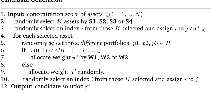
Candidate Generation

1.Input:concentration score of assetsci(i= 1, ..., N)

2. randomly selectKassets byS1,S2,S3orS4.

3. randomly select an indexifrom thoseKselected and assignitojandχ

4. foreach selected asset

5. randomly select threedifferentportfolios: p1,p2,p3∈P

6. if r(0,1)< CR || j==χ

7. allocate weightw0byW1,W2orW3

8. else

9. allocate weightw0randomly.

10. randomly select an indexifrom thoseKselected and assignitoj

12.Output:candidate solutionp0.

Figure 3: The procedure of generating a candidate solution.

4.6. Constraint handling

When using an evolutionary algorithm to solve constrained optimization problems, there are various methods proposed in the literature [15] for han-dling constraints in evolutionary optimization, such as penalty function method, special representations and operators, repair methods and multi-objective meth-ods. Among those methods, repair method is one of the effective approaches to locate feasible solutions.

During the population sampling, each constructed individual portfolio is re-paired if it does not satisfy all considered constraints. As described in Section 4.5, the new solution generated by our proposed MODEwAwL already satisfies the cardinality and pre-assignment constraints.

Hence, the following repair mechanism stated in [50,54] is applied:

1. All weights of selected assets in the candidate solution are adjusted by settingw0_i=i+

w0 i−i

P_(w0 i−i).

2. The weights are then adjusted to the nearest round lot level by setting

w0_i=w_i0−(w_i0 mod υi). The remaining amount of capital is redistributed

in such a way that the largest amount of (w0_i mod υi) is added in lot of

υiuntil all the capital is spent.

4.7. Selection scheme

The proposed MODEwAwL applies the elitist selection scheme based on Pareto optimality (see Fig.2). During the evolution, the population is extended by adding the newly found non-dominated solutions. Hence, at each genera-tion, the number of portfolios in the current population will be betweenN P

4.8. Truncate population

In each generation, if the number of portfolios in the current population exceeds its limit N P, it needs to identify those which need to be removed. The individuals in the population are sorted based on the non-dominance and crowding distance measures. Then the current population is truncated by keep-ing the bestN P individuals for the next generation.

4.9. Maintaining the external archive

The main objective of the external archiveAis to keep all the non-dominated solutions encountered along the search process. This approach is adopted in order to save and update all well spread non-dominated solutions generated by the algorithm during the search.

In each generation, the archive A is updated with the non-dominated so-lutions from the trial population. The computational time of maintaining the archive increases with the archive size [14, 32, 60]. The size of the archive is therefore restricted to a pre-specified value. When the external archive has reached its maximum capacityM, the crowding distances of the solutions are calculated to determine the most crowded archive members which need to be discarded.

5. Performance evaluation

In this section, we first introduce the test problems and performance metrics used for evaluating the proposed MODEwAwL. We then study the effectiveness of the two components extended for MODEwAwL, i.e. the external archive and the learning-guided solution generation scheme, respectively. Finally, we compare the proposed MODEwAwL with four state-of-the-art multi-objective evolutionary algorithms in terms of the performance metrics.

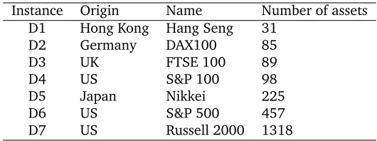
5.1. Dataset

Seven test problems based on well-known major market indices for the port-folio optimization problems from the publicly available OR-library [4] is used to evaluate the performance of the algorithms. Table1 shows the details of these benchmark indices and their sizes. The first five datasets (D1 – D5) built from weekly price data from March 1992 to September 1997 are available at:

http://people.brunel.ac.uk/~mastjjb/jeb/orlib/portinfo.html.

They were first introduced by Chang et al [11].

The remaining two datasets were built based on the index tracking problem and they were first introduced by Canakgoz and Beasley [9]. These two datasets (D6 and D7) are available at:

http://people.brunel.ac.uk/~mastjjb/jeb/orlib/indtrackinfo.html.

Instance Origin Name Number of assets

D1 Hong Kong Hang Seng 31

D2 Germany DAX100 85

D3 UK FTSE 100 89

D4 US S&P 100 98

D5 Japan Nikkei 225

D6 US S&P 500 457

D7 US Russell 2000 1318

Table 1: The benchmark instances from OR-library.

5.2. Quality indicators

To evaluate the performance of the multi-objective evolutionary algorithms from various aspects, several performance metrics have been proposed in the literature which mainly consider proximity, diversity and distribution. In this study we use four widely adopted performance evaluation metrics namely gen-erational distance, inverted gengen-erational distance, diversity and hypervolume.

5.2.1. Inverted generational distance (IGD)

The inverted generational distance [48] uses the true Pareto front as a ref-erence and measures the distance of each of its elements from the true Pareto front to the non-dominated front obtained by an algorithm. It is mathematically defined as:

IGD=

s

Q

P

i=1

d2

i

Q

whereQ is the number of solutions in the true Pareto front anddi is the

Eu-clidean distance between each of the solution and the nearest member from the set of non-dominated solutions found by the algorithm. This metric measures both the diversity and the convergence of an obtained non-dominated solution set. The smaller the value of this metric, the closer the obtained front is to the true Pareto front.

The true Pareto front for highly constrained multi-objective portfolio opti-mization problem considered in this work is unknown. We use the best known unconstrained efficient frontier (UCEF) provided by the OR-library [4] as the true Pareto front reference set. This has been widely adopted in the literature.

5.2.2. Generational distance (GD)

5.2.3. Diversity metric (∆)

The diversity metric (∆) [19] measures the performance indices of distribu-tion and spread simultaneously for two-objective optimizadistribu-tion problems. The diversity metric (∆) is defined as follows:

∆ =

df+dl+

|Q|−1

P

i=1

|di−d|

df+dl+ (|Q| −1)d

wheredi is the Euclidean distance in the objective space between consecutive

solutions in the obtained non-dominated frontQ, andd¯is the average of these distances. The parametersdf anddl are the Euclidean distance between the

extreme solutions and the boundary solutions of the obtained non-dominated frontQ. The lower value of the spread (∆) indicates a better diversity.

5.2.4. Hypervolume (HV)

Hypervolume metric [61], also known as S-metric or Lebesgue measure, is widely recognized as a unary value which is able to measure both convergence and diversity. This metric calculates the normalized volume of the objective space covered by the obtained Pareto set Q bounded by a reference point r. Therefore, higher values are preferable. For each solutioni∈Q, a hypercubeci

from solutioniand the reference pointris measured. The hypervolume HV is calculated as:

HV =volume(∪|_iQ₌₁|ci)

An accurate calculation of HV requires a normalized objective space and we used the linear normalization technique proposed by Knowles et al [31] as fol-lows:

fi=

fi−fimin

fmax i −fimin

where fmin

i and fimax are the minimum and maximum value of the ith

ob-jective. The value offmin

i andfimax are set as the minimum and maximum

value obtained from running all algorithms. The reference point was chosen as r={1,0}.

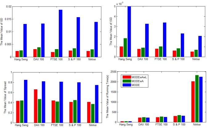
5.3. Effectiveness of the learning-guided solution generation and archive

Figure 4: Effectiveness of the learning-guided solution generation scheme and archive.

5.4. The Overall Performance Evaluation

In order to evaluate the overall performance of the proposed MODEwAwL, we compare it with four state-of-the-art multi-objective evolutionary algorithms in the literature.

• NSGA-II: the Non-dominated Sorting Genetic Algorithm II was proposed by Deb et al. [19]. The algorithm uses binary tournament selection based on the crowding distance. It performs crossover and mutation by simu-lated binary crossover and polynomial mutation operators.

• SPEA2: the Strength Pareto Evolutionary Algorithm was proposed by Zit-zler et al. [60]. The algorithm employs fine-grained fitness assignment, density estimation techniques and archive truncation methods. Like NSGA-II, it uses binary tournament selection, simulated binary crossover and polynomial mutation evolutionary operators.

• PESA2: the Pareto Envelope-based Evolutionary Algorithm was proposed by Corne et al. [16]. The algorithm uses hyper-boxes to assign fitness and employs the simulated binary crossover and polynomial mutation opera-tions.

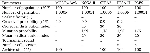
In order to ensure a fair comparison, we have used the same population size and archive size (if applicable) for all the algorithms tested in this work. We have chosen to run all the algorithms run for the same stopping criteria (i.e. the same number of evaluations) to generate the Pareto front. Each algorithm also uses the same encodings (see Section4.2) and repair mechanism (see Section4.6) when a newly constructed portfolio violates the considered constraints. Before the experiments were performed, parameters are tuned for all algorithms using the smallest problem instance, i.e. Hang Seng. Table2shows the best parameter values of the algorithms.

Parameters MODEwAwL NSGA-II SPEA2 PESA-II PAES Number of population (N P) 100 100 100 100 100 Number of generation 1,000N 1,000N 1,000N 1,000N 1,000N

Scaling factor (F) 0.3 – – – –

Crossover probability (CR) 0.9 0.9 0.9 0.9 – Crossover distribution index – 20 20 20 – Mutation probability – 1/N 1/N 1/N 1/N Mutation distribution index – 20 20 20 20

Tournament round – – 1 – –

Number of bisection – – – 5 5

Archive size (M) 100 – 100 100 100

Table 2: Parameter setting of five algorithms.

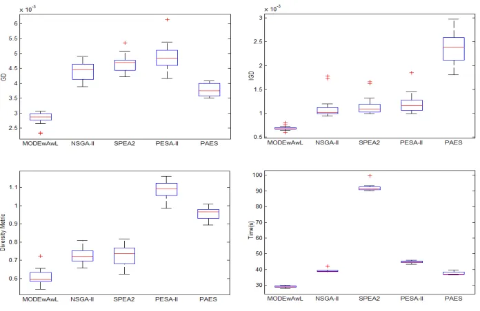
Figure 6: Performance comparisons of five algorithms in term of GD, IGD and∆metrics for DAX 100 dataset.

Figure 8: Performance comparisons of five algorithms in term of GD, IGD and∆metrics for S & P 100 dataset.

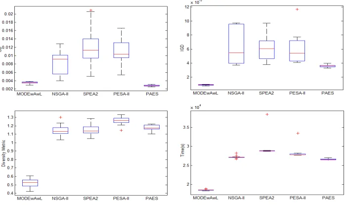
Figure 10: Performance comparisons of five algorithms in term of GD, IGD and∆metrics for S & P 500 dataset.

5.5. Comparisons of the algorithms

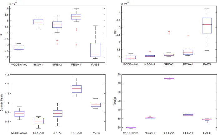
In this section, we have performed a number of experiments. The results of GD, IGD and∆and running time of the five algorithms performed on seven datasets from OR-library are shown in Figs. [5,6,7,8,9,10,11]. For example in Fig. 11, top left boxplot represents the performance of each algorithm con-sidered in terms of GD metric, top right boxplot represents the performance of each algorithm considered in terms of IGD metric, bottom left shows the perfor-mance of each algorithm in terms of Diversity metric and bottom right boxplot displays the computational time for each algorithm considered. These results are obtained for the constrained portfolio optimization problem with cardinality

K= 10, floori = 0.01, ceilingδi= 1.0, pre-assignmentz30= 1and round lot

υi= 0.008.

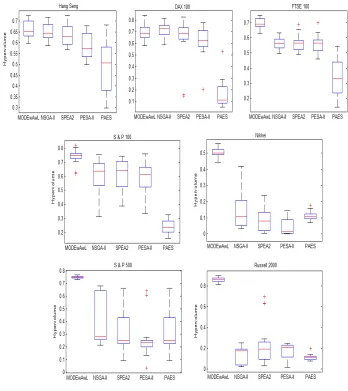
The results show that for most of the problem instances, the MODEwAwL obtains the smallest mean values for GD, IGD and ∆ , compared with the other four algorithms, demonstrating the best performance among the five al-gorithms. NSGA-II comes at the second and SPEA2 comes at the third places. NSGA-II and SPEA2 seem to have almost comparable results for most problem instances. However, SPEA2 is the most computationally expensive algorithm in terms of CPU time. The results also confirm that PAES is the worst algorithm for the portfolio optimization with considered constraints. However, PAES is the second fastest algorithm after MODEwAwL. For most of the problem instances, the proposed algorithm MODEwAwL is also computationally efficient compared to the others. Fig. 12shows the hypervolume (HV) calculation performed on seven datasets and for each problem instance, the results reconfirm the superi-ority of MODEwAwL since it outperforms in six out of seven datasets.

For illustrative purpose, the obtained efficient frontiers of the algorithms for seven instances along with the true unconstrained efficient frontier (UCEF) are provided in Fig. 13. When the problem sizes are small, the Pareto sets obtained by the considered algorithms are very competitive to each other such that it would be hard to differentiate visually. As the problem sizes increase, the proposed algorithm obtained significantly better efficient frontier than those obtained by other MOEAs considered in this work. Based on the analysis, we conclude that the proposed MODEwAwL is able to solve large-scale real-world portfolio optimization efficiently. The results also demonstrate that NSGAII and SPEA2 loose their effectiveness when the problem dimension increases.

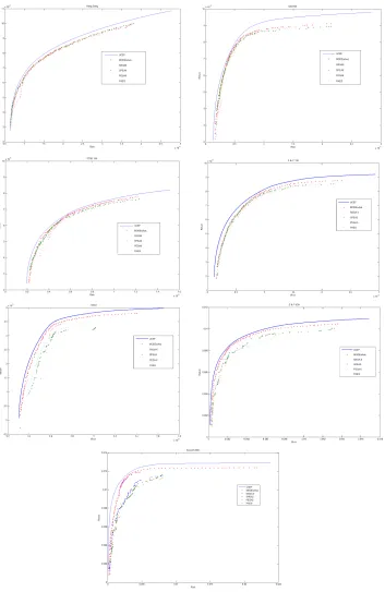
To gain an intuitive view of the five algorithms over generations, we plot the GD, IGD and∆metrics over generations on five selected instances in Fig. 14where the results are averaged over 20 runs. The results confirm that all algorithms considered are able to converge and MODEwAwL is able to converge the fastest in most problem instances.

Experiments are also performed for different cardinality values withK= 15

andK= 5. The results are made publicly accessible at:

http://cs.nott.ac.uk/~ktl/results/MODEwAwL-results.pdf. On the

Figure 12: Performance comparisons of five algorithms in term of HV metric.

algorithm is efficient for various search spaces with different values ofK. The proposed MODEwAwL is thus more robust than the compared MOEAs.

Algorithm1↔Algorithm2 Hang Seng DAX 100 FTSE 100 S & P 100 Nikkei S & P 500 Russell 2000

MODEwAwL↔NSGA-II ∼ + + + + + +

MODEwAwL↔SPEA2 − + + + + + +

MODEwAwL↔PESA-II ∼ + + + + + +

MODEwAwL↔PAES + + + + + + +

NSGA-II↔SPEA2 − + ∼ ∼ + + ∼

NSGA-II↔PESA-II + + + ∼ + + ∼

NSGA-II↔PAES + + + + ∼ + −

SPEA2↔PESA-II + ∼ ∼ ∼ + ∼ ∼

SPEA2↔PAES + + + + − ∼ −

PESA-II↔PAES + + + + − ∼ −

Table 3: Student’s t-test results of different algorithms on seven problem instances with K=10, i= 0.01,δi= 1.0,z30= 1andυi= 0.008.

statistical results obtained by a two-tailed t-test with 38 degrees of freedom at a 0.05 level of significance are given in Table [3,4,5]. The result of Algorithm-1

↔Algorithm-2 is shown as “+”, “−”, or “∼” when Algorithm-1 is significantly better than, significantly worse than, or statistically equivalent to Algorithm-2, respectively. Results show that MODEwAwL outperforms other algorithms in most of the problem instances except Hang Seng dataset. For Hang Seng test problem, the performance of SPEA2 outperforms MODEwAwL whenK = 10. We therefore can conclude that the proposed MODEwAwL has the best opti-mization performance for the portfolio optiopti-mization problem with considered constraints.

Algorithm1↔Algorithm2 Hang Seng DAX 100 FTSE 100 S & P 100 Nikkei S & P 500 Russell 2000

MODEwAwL↔NSGA-II ∼ + + + + + +

MODEwAwL↔SPEA2 ∼ + + + + + +

MODEwAwL↔PESA-II + + + + + + +

MODEwAwL↔PAES + + + + + + +

NSGA-II↔SPEA2 + ∼ + + + ∼ ∼

NSGA-II↔PESA-II + + + + + ∼ ∼

NSGA-II↔PAES + + + + + + ∼

SPEA2↔PESA-II + ∼ ∼ ∼ + ∼ ∼

SPEA2↔PAES + + + + − ∼ ∼

PESA-II↔PAES + + + + − ∼ ∼

Table 4: Student’s t-test results of different algorithms on 5 problem instances with K=15,i= 0.01,

δi= 1.0,z30= 1andυi= 0.008.

Algorithm1↔Algorithm2 Hang Seng DAX 100 FTSE 100 S & P 100 Nikkei S & P 500 Russell 2000

MODEwAwL↔NSGA-II + + + + + + +

MODEwAwL↔SPEA2 + + + + + + +

MODEwAwL↔PESA-II + + + + + + +

MODEwAwL↔PAES + + + + + + +

NSGA-II↔SPEA2 − + ∼ + + ∼ ∼

NSGA-II↔PESA-II + + ∼ + + ∼ ∼

NSGA-II↔PAES + + + + − − −

SPEA2↔PESA-II + ∼ ∼ ∼ + ∼ ∼

SPEA2↔PAES + + ∼ ∼ − − −

PESA-II↔PAES ∼ + ∼ + − − −

6. Conclusion and future work

In this work, we investigated the portfolio selection problem with four prac-tical constraints which limit the number of assets in a portfolio, restrict the min-imum and maxmin-imum proportions of assets held in the portfolio, require some specific assets to be included in the portfolio and require to invest the assets in units of a certain size respectively.

We have demonstrated that maintaining a secondary population of solution set in combination with learning-guided candidate solution generation scheme contribute to better performance over four existing well-known MOEAs, NSGA-II, SPEA2, PEAS-II and PAES. The experimental results not only show that the quality of the generated Pareto set approximations significantly improved, but also that the overall computation time can be reduced. As to the Pareto set approximation, the proposed solution generation scheme embedding learning mechanism, problem specific heuristics and direction-based search methods plays a major role, while the efficiency is mainly because the proposed algorithm is computationally cheap as it only uses a single update at each generation. Per-formance wise, the proposed MODEwAwL algorithm is not only capable to de-liver high-quality portfolios enriched with additional constraints but also able to efficiently solve a reasonable size of asset up to 1318. The proposed algorithm could be applied to other practical applications such as knapsack problems with relevant constraints. For future work, the proposed algorithm can be extended to include constraints such as transaction cost and short selling.

Acknowledgements

This research was supported by the School of Computer Science, The Univer-sity of Nottingham. The authors would also like to thank anonymous reviewers for their helpful comments.

References

[1] K. Anagnostopoulos and G. Mamanis. A portfolio optimization model with three objectives and discrete variables. Computers & Operations Research, 37(7):1285–1297, 2010.

[2] K. Anagnostopoulos and G. Mamanis. The mean–variance cardinality con-strained portfolio optimization problem: an experimental evaluation of five multiobjective evolutionary algorithms. Expert Systems with Applica-tions, 38(11):14208–14217, 2011.

[3] R. Armananzas and J. A. Lozano. A multiobjective approach to the port-folio optimization problem. In The 2005 IEEE Congress on Evolutionary Computation, volume 2, pages 1388–1395. IEEE, 2005.

[5] D. Bertsimas and R. Shioda. Algorithm for cardinality-constrained quadratic optimization. Computational Optimization and Applications, 43(1):1–22, 2009.

[6] D. Bienstock. Computational study of a family of mixed-integer quadratic programming problems. Mathematical programming, 74(2):121–140, 1996.

[7] J. Branke, B. Scheckenbach, M. Stein, K. Deb, and H. Schmeck. Portfolio optimization with an envelope-based multi-objective evolutionary algo-rithm. European Journal of Operational Research, 199(3):684–693, 2009.

[8] R. Brito and L. Vicente. Efficient Cardinality/Mean-Variance Portfolios. 2012.

[9] N. Canakgoz and J. E. Beasley. Mixed-integer programming approaches for index tracking and enhanced indexation.European Journal of Operational Research, 196(1):384–399, 2009.

[10] M. Castillo Tapia and C. Coello. Applications of multi-objective evolution-ary algorithms in economics and finance: a survey. In IEEE Congress on Evolutionary Computation, 2007. CEC 2007, pages 532–539. IEEE, 2007.

[11] T. Chang, N. Meade, J. Beasley, and Y. Sharaiha. Heuristics for cardinality constrained portfolio optimisation. Computers and Operations Research, 27(13):1271–1302, 2000.

[12] S. Chiam, K. Tan, and A. Al Mamum. Evolutionary multi-objective portfo-lio optimization in practical context. International Journal of Automation and Computing, 5(1):67–80, 2008.

[13] C. Coello. Evolutionary multi-objective optimization and its use in finance. Handbook of Research on Nature Inspired Computing for Economy and Man-agement. Idea Group Publishing, 2006.

[14] C. A. C. Coello, G. T. Pulido, and M. S. Lechuga. Handling multiple objec-tives with particle swarm optimization. Evolutionary Computation, IEEE Transactions on, 8(3):256–279, 2004.

[15] C. A. Coello Coello. Theoretical and numerical constraint-handling tech-niques used with evolutionary algorithms: a survey of the state of the art. Computer methods in applied mechanics and engineering, 191(11):1245– 1287, 2002.

[17] T. Cura. Particle swarm optimization approach to portfolio optimization. Nonlinear Analysis: Real World Applications, 10(4):2396–2406, 2009.

[18] K. Deb. Multi-objective optimization. Multi-objective Optimization Using Evolutionary Algorithms, pages 13–46, 2001.

[19] K. Deb, A. Pratap, S. Agarwal, and T. Meyarivan. A fast and elitist mul-tiobjective genetic algorithm: NSGA-II. IEEE Transactions on Evolutionary Computation, 6(2):182–197, 2002.

[20] G. Deng, W. Lin, and C. Lo. Markowitz-based portfolio selection with car-dinality constraints using improved particle swarm optimization. Expert Systems with Applications, 2011.

[21] G. Di Tollo and A. Roli. Metaheuristics for the portfolio selection problem. International Journal of Operations Research, 5(1):13–35, 2008.

[22] L. Diosan. A multi-objective evolutionary approach to the portfolio op-timization problem. In Computational Intelligence for Modelling, Control and Automation, 2005 and International Conference on Intelligent Agents, Web Technologies and Internet Commerce, International Conference on, vol-ume 2, pages 183–187. IEEE, 2005.

[23] J. E. Fieldsend, J. Matatko, and M. Peng. Cardinality constrained portfo-lio optimisation. InIntelligent Data Engineering and Automated Learning– IDEAL 2004, pages 788–793. Springer, 2004.

[24] C. Fonseca and P. Fleming. An overview of evolutionary algorithms in multiobjective optimization. Evolutionary computation, 3(1):1–16, 1995.

[25] L. D. Gaspero, G. D. Tollo, A. Roli, and A. Schaerf. Hybrid metaheuris-tics for constrained portfolio selection problems. Quantitative Finance, 11(10):1473–1487, 2011.

[26] N. Gulpinar, L. T. H. An, and M. Moeini. Robust investment strategies with discrete asset choice constraints using dc programming. Optimiza-tion, 59(1):45–62, 2010.

[27] M. Hirschberger, Y. Qi, and R. E. Steuer. Large-scale MV efficient fron-tier computation via a procedure of parametric quadratic programming. European Journal of Operational Research, 204(3):581–588, 2010.

[28] C. Israelsen. The benefits of low correlation.Journal of Indexes, 10(6):18– 26, 2007.

[30] J. Knowles and D. Corne. The Pareto archived evolution strategy: a new baseline algorithm for pareto multiobjective optimisation. InProceedings of the 1999 Congress on Evolutionary Computation, 1999. CEC 99, vol-ume 1. IEEE, 1999.

[31] J. Knowles, L. Thiele, and E. Zitzler. A Tutorial on the Performance Assess-ment of Stochastic Multiobjective Optimizers. No. 214, Computer Engi-neering and Networks Laboratory (TIK), ETH Zurich, Switzerland, 2006. (revised version).

[32] J. D. Knowles and D. W. Corne. Approximating the nondominated front using the Pareto archived evolution strategy. Evolutionary computation, 8(2):149–172, 2000.

[33] G. A. Kochenberger et al. Handbook of Metaheuristics. Springer, 2003.

[34] T. Krink and S. Paterlini. Multiobjective optimization using differential evolution for real-world portfolio optimization. Computational Manage-ment Science, 8(1-2):157–179, 2011.

[35] D. Li, X. Sun, and J. Wang. Optimal lot solution to cardinality constrained mean–variance formulation for portfolio selection. Mathematical Finance, 16(1):83–101, 2006.

[36] C.-C. Lin and Y.-T. Liu. Genetic algorithms for portfolio selection problems with minimum transaction lots.European Journal of Operational Research, 185(1):393–404, 2008.

[37] K. Lwin and R. Qu. A hybrid algorithm for constrained portfolio selection problems. Applied Intelligence,DOI:10.1007/s10489-012-0411-7, 2013.

[38] R. Mansini and M. G. Speranza. Heuristic algorithms for the portfolio selection problem with minimum transaction lots. European Journal of Operational Research, 114(2):219–233, 1999.

[39] D. Maringer. Portfolio Management with Heuristic Optimization, volume 8. Springer Verlag, 2005.

[40] H. Markowitz. Portfolio selection.The Journal of Finance, 7(1):pp. 77–91, 1952.

[41] H. Markowitz. Portfolio Selection: Efficient Diversification of Investments. John Wiley and Sons, New York, 1959.

[42] S. Mishra, G. Panda, S. Meher, R. Majhi, and M. Singh. Portfolio manage-ment assessmanage-ment by four multiobjective optimization algorithm. InRecent Advances in Intelligent Computational Systems (RAICS), 2011 IEEE, pages 326–331. IEEE, 2011.

[44] A. Ponsich, A. Jaimes, and C. Coello. A survey on multiobjective evolu-tionary algorithms for the solution of the portfolio optimization problem and other finance and economics applications. IEEE Transactions on Evo-lutionary Computation, 17(3):321–344, 2013.

[45] G. R. Raidl. A unified view on hybrid metaheuristics. InHybrid Meta-heuristics, pages 1–12. Springer, 2006.

[46] T. Robiˇc and B. Filipiˇc. DEMO: differential evolution for multiobjective optimization. In Evolutionary Multi-Criterion Optimization, pages 520– 533. Springer, 2005.

[47] D. X. Shaw, S. Liu, and L. Kopman. Lagrangian relaxation procedure for cardinality-constrained portfolio optimization. Optimisation Methods & Software, 23(3):411–420, 2008.

[48] M. R. Sierra and C. A. C. Coello. Improving PSO-based multi-objective op-timization using crowding, mutation and epsilon-dominance. InEMO’05, pages 505–519, 2005.

[49] P. Skolpadungket and K. Dahal. A survey on portfolio optimisation with metaheuristics. SKIMA 2006, page 103, 2006.

[50] P. Skolpadungket, K. Dahal, and N. Harnpornchai. Portfolio optimization using multi-obj ective genetic algorithms. InIEEE Congress on Evolutionary Computation, 2007. CEC 2007, pages 516–523. IEEE, 2007.

[51] E. D. Smith, Y. J. Son, M. Piattelli-Palmarini, and A. Terry Bahill. Ameliorating mental mistakes in tradeoff studies. Systems Engineering, 10(3):222–240, 2007.

[52] M. Stein, J. Branke, and H. Schmeck. Efficient implementation of an active set algorithm for large-scale portfolio selection. Computers & Operations Research, 35(12):3945–3961, 2008.

[53] R. Storn and K. Price. Differential Evolution–a simple and efficient adap-tive scheme for global optimization over continuous spaces. Technical Report TR-95-012, Berkeley, CA, 1995.

[54] F. Streichert, H. Ulmer, and A. Zell. Evaluating a hybrid encoding and three crossover operators on the constrained portfolio selection prob-lem. InCongress on Evolutionary Computation, 2004. CEC2004, volume 1, pages 932–939. IEEE, 2004.

[55] F. Streichert, H. Ulmer, and A. Zell. Evolutionary algorithms and the cardi-nality constrained portfolio optimization problem. InOperations Research Proceedings 2003, pages 253–260. Springer, 2004.

[57] D. A. Van Veldhuizen and G. B. Lamont. Multiobjective evolutionary algo-rithm research: a history and analysis. Technical report, Citeseer, 1998.

[58] R. E. Walpole, R. H. Myers, S. L. Myers, and K. Ye.Probability and Statistics for Engineers and Scientists, volume 8. Prentice Hall Upper Saddle River, NJ:, 1998.

[59] E. Zitzler, K. Deb, and L. Thiele. Comparison of multiobjective evolution-ary algorithms: empirical results. Evolutionary computation, 8(2):173– 195, 2000.

[60] E. Zitzler, M. Laumanns, L. Thiele, E. Zitzler, E. Zitzler, L. Thiele, and L. Thiele. Spea2: Improving the Strength Pareto Evolutionary Algorithm, 2001.