Numerical Approximation of Real Finite Nonnegative Function by the Modulus of Discrete Fourier Transform

doi:10.4236/am.2010.11008 Published Online May 2010 (http://www.SciRP.org/journal/am)

Numerical Approximation of Real Finite Nonnegative

Function by the Modulus of Discrete Fourier

Transform

Petro Savenko, Myroslava Tkach

Pidstryhach Institute for Applied Problems of Mechanics and Mathematics, National Academy of Sciences of Ukraine, Lviv, Ukraine

Email:{spo, tmd}@iapmm.lviv.ua

Received March 15, 2010; revised April 21, 2010; accepted April 28, 2010

Abstract

The numerical algorithms for finding the lines of branching and branching-off solutions of nonlinear prob-lem on mean-square approximation of a real finite nonnegative function with respect to two variables by the modulus of double discrete Fourier transform dependent on two parameters, are constructed and justified.

Keywords:Mean-Square Approximation, Discrete Fourier Transform, Two-Dimensional Nonlinear Integral Equation, Nonuniqueness And Branching of Solutions.

1. Introduction

The mean-square approximation of real finite nonnega-tive function with respect to two variables by the mod-ulus of double discrete Fourier transform dependent on physical parameters, is widely used, in particular, at modeling and solution of the synthesis problems of dif-ferent types of antenna arrays, signal processing etc. [1-3]. Nonuniqueness and branching of solutions are essential features of nonlinear approximation problem which remains unexplored. The problem on finding the set of branching points, in turn, is not adequately ex-plored nonlinear spectral two-parametric problem. The methods of investigation and numerical finding the solu-tions of one-parametric spectral problems at presence of discrete spectrum [4-8] are most well-developed. The existence of coherent components of spectrum, which are spectral lines for the case of real parameters [9], is essen-tial difference of nonlinear two-parametric spectral problems.

In the work a variational problem on the best mean- square approximation of a real finite nonnegative func-tion by the module of double discrete Fourier transform is reduced to finding the solutions of Hammerstein type nonlinear two-dimensional integral equation. Using the Schauder principle the existence of solutions is proved. The existence theorem of coherent components of spec-trum of holomorphic matrix functions dependent on two spectral parameters is proved. It justifies the application of implicit functions methods to multiparametric spectral problems [9]. The applicability of this theorem to the

analysis of spectrum of two-dimensional integral homo-geneous equation to which is reduced the problem on finding the lines of possible branching of solutions of the Hammerstein equation, is shown. Algorithms for numer-ical finding the optimum solutions of an approximation problem are constructed and justified. Numerical exam-ples are presented.

2. Problem Formulation, Basic Equations

and Relations

Consider the special case of double discrete Fourier transform

(

)

2 2

1 1 ( )

1 2 1 1 2 2

( )

( , ) exp

N M n

nm nm nm

n N m M n

f s s I i c x s c y s

=− =−  

=

∑ ∑

_ % +% _

setting here x_nm = ∆n _x (n= − ÷N N) , ynm = ∆m y

(m= − ÷M M); c1= ∆c%1 x, c2= ∆c%2 y. If it is necessary

for the accepted assumptions we shall consider the for-mula

(

)

1 2 1 1 2 2

( , ) exp

N M

nm n N m M

f s s A I i c ns c ms

=− =−

= I≡

∑ ∑

_ + _ (1)

as a linear operator, acting from complex finite-dimensional space N2 M2

I

H =£ × ₍N₂=2N+1_, M₂=2M+1) into the space of complex-valued continuous functions with respect to two real variables determined in the domain

(

)

{

s s1, 2 : s1 c1, s2 c2

}

Here c1, c2 are any real non-dimensional numerical

parameters belonging to

(

)

{

1, 2 : 0 1 , 0 2

}

c c c c a c b

Λ = < ≤ < ≤ .

The function f s s( ,1 2) is 2π c1 - periodic function

on argument s₁ and 2π c₂ - periodic on s₂.

In considered spaces we introduce scalar products and generable by them norms

(

1 2

)

2

1 2

4 ,

I

N M

nm nm H

n N m M I I c c =− =−

π

=

∑ ∑

I I ,

( )

1/ 2

,

I H

=

I I I , (2)

(

)

( )( 2)

(

) (

)

1, 2 C 1 1, 2 2 1, 2 1 2

f f f s s f s s ds ds

Ω =

∫∫

_Ω

,

(

)

_{( )}( 2) 1/ 2

, _C

f f f

Ω

= . (3) Denote an augmented space of continuous functions with entered scalar product and norm (3) as C(2)_{( )Ω} and notice that its augmentation coincides with the Hilbert space L₂( )Ω [10].

By direct check we are sure that such equality

(

)

2 2 2

2

1 2 1 2

,

, nm

n m

AI f s s ds ds I I

Ω

=

_∫∫

=

∑

= (4)

is valid. From here follows, that A is isometric opera-tor in sense (4).

Using the entered scalar products (2) and (3) we find the conjugate operator required later on

(

)

(

)

1 2

1 2 1 1 2 2 1 2

2 , exp

4

c c

A f∗ f s s i c ns c ms ds ds

Ω

= _− + _

π

∫∫

(

n= − ÷N N m, = − ÷M M

)

. (5) Let such function be given

1 2 1 2

1 2

1 2

( , ), ( , ) ,

( , )

0, ( , ) \ ,

F s s s s G

F s s

s s G

 ∈ ⊆ Ω



=  _∈Ω



% (6)

where F s s( ,_{1 2}) is a real continuous and nonnegative in the domain G function.

Consider a problem on the best mean-square approxi-mation of the function F s s( ,1 2) in the domain Ω by

the module of double discrete Fourier transform (1) ow-ing to select of coefficients of the vector I. We shall formulate it as a minimization problem of the functional

( )( 2) ( )( 2)

2 2

( ) F A F f

C C

I I

Ω Ω

σ = − ≡ − (7)

in the Hilbertian space HI. Taking into account (4) and

(5), we write the functional σ( )I in a simplified form

( )

(

)

( )

( 2) ( 2) 2

2 2

( ) 2 ,

I H

F F A

C C

I I I

Ω Ω

σ = − + . (8)

On the basis of necessary condition of functional minimum we obtain a nonlinear system of equations re-lating to the components of vector I in the space H_I

that are represented in the vector and expanded forms, respectively:

( )

{

exp arg

}

A F i A

I= ∗ _ I _ , (9)

(

)

1 2

1 2

2 , exp arg

4

N M

nm nm

k N l M c c

I F s s i I

=− =− Ω

  



= _{  } ×

π

∫∫

_{  }

∑ ∑

(

1 1 2 2

)

)

(

1 1 2 2

)

}

1 2

exp i c ks c ls c ns c ms  ds ds

× _ + _ − + _

(

n= − ÷N N m, = − ÷M M

)

. (9′) Acting on both parts of (9) by operator A we obtain equivalent to (9) the Hammerstein type nonlinear integral equation relating to f :

(

)

[

]

( ) , , ( ) exp arg ( )

f Q Bf K Q Q c F Q i f Q dQ

Ω

′ ′ ′ ′

= ≡

_∫∫

, (10)

where Q′=( ,s s1′ ′2),dQ′=ds ds1′ ′2,c=

(

c c1, 2

)

;

(

, ,

)

1

(

1, 1, 1

)

2

(

2, 2, 2

)

K Q Q′c =K s s c′ ⋅K s s c′ , (11)

(

)

1

(

)

1 1, 1, 1 exp 1 1 1

2

N

n N c

K s s c ic n s s

=−

′ = _ − ′ _≡

π

∑

(

)

(

)

2 1 1 1 1

1

1 1

sin 2 2

2

N c

s s

c c

s s

 _{− ′} 

 

 

≡

π _{− ′} ,

(

)

2

(

)

2 2, 2, 2 exp 2 2 2

2

M

m M c

K s s c ic m s s

=−

′ = _ − ′ _≡

π

∑

(

)

(

)

2 2

2 2

2 2

2 2

sin 2 2

2

M c

s s

c c

s s

 _{− ′} 

 

 

≡

π _{− ′} .

Note, that the kernel (11) of Equation (10) is degene-rate and real.

We shall consider one of the properties of function

(

)

exp iarg (f Q′) entering into (10) at f Q( ′ →) 0. Ob-viously that the function

(

)

(

_{2 2}

)

1 2

( ) ( ) ( )

exp arg ( )

( ) _{( ) ( )}

f Q u Q iv Q

i f Q

f Q _{u Q v Q}

′ ′ + ′

′ = ≡

′ _{′ + ′}

is continuous if u Q( ′)=Re (f Q′) and v Q( ′)=Im (f Q′) ( ) Im ( )

v Q′ = f Q′ are continuous functions, where exp

(

iarg (f Q) 1

)

complex zero [11, p. 20]. On this basis we redefine

(

)

exp iarg (f Q′) at u Q( ′ →) 0 and v Q( ′ →) 0 as a function which has module equal to unit and undeter-mined argument.

The equivalence of (9) and (10) follows from the fol-lowing lemma.

Lemma 1. Between solutions of Equations (9) and (10)

there exists bijection, i.e., if I_∗ is a solution of (9) then f_∗=AI_∗ is the solution of (10); on the contrary, if f_∗ is the solution of (10) then

[

]

{

exp arg( )

}

A F i f

I_∗= ∗ _∗ (12)

is the solution of (9).

Proof. Let I_∗ be a solution of (9). Then I_∗−A∗ F i AI_∗ ≡

( )

{

exp arg

}

0

A∗ F i A

∗−  ∗  ≡

I I . Acting on this identity by the

linear operator A, we have AI_∗−AA∗

{

Fexp_iarg

(

AI_∗ _ ≡0

( )

}

exp arg 0

AI_∗−AA F _i AI_∗ _ ≡ . Since the operator A acts from the space

2 2 N M I

H =£ × into the space C(2)( )Ω and accordingly into

the space H%f =L2( )Ω , and the set of its nulls consists

of only null element from the last identity follows, what

f

AI_∗= ∈f_∗ H% is a solution of (10).

On the contrary, let f_∗∈H%_f solves the Equation (10). The operator A∗ acts from the space H%∗_f =L∗₂( )Ω into the space N2 M2

I

H =£ × [10] and the Hilbertian space L∗₂ coincides with the space L₂ [10]. From here follows, that A∗ acts from the space H%_f =L₂( )Ω into the space N2 M2

I

H =£ × . Taking into account that F is a finite function determined by (6), and f_∗ is conti-nuous, the function Fexp

(

iarg(f_∗)

)

is quadratic inte-grability in the domain Ω, i.e. Fexp arg(

(

i f∗)

)

∈Hf.

Thus A

(

Fexp

(

iarg(f )

)

)

HI

∗

∗ = ∈I∗ and the right part

of (10) is the result of action of operator A on an ele-ment I_∗, i.e. AI_∗=AA∗

(

Fexp arg(

(

i f_∗)

)

)

= f_∗. Writ-ing this equality as A

(

I_∗−A∗

(

Fexp

(

iarg(AI_∗)

)

)

)

=0 and taking into account that a set of operator nulls con-sists of only a null element we obtain

(

)

(

exp arg( )

)

A F i A

I_∗= ∗ I_∗ . So, I_∗= A∗

(

Fexp

(

iarg(f_∗)

)

)

exp arg( )

A F i f

∗ ∗ solves the Equation (9). Lemma is proved.

Thus owing to the equivalence of (9) and (10) we con-sider simpler of them, namely (10). The Equation (9) is a more complicated equation in sense that in its right part the operator A is in an index of the power of exponent.

Besides taking into account that a set of values of opera-tor A is a set of continuous functions in the domain

Ω belonging to the space L2

( )

Ω and this set is a

compact in the space L2( )Ω [12], we shall investigate

solutions of (10) in the space C( )Ω .

Formulate the important properties of (10), which are checked directly.

1) If function f Q( ) is a solution of (10) then the conjugate complex function f Q( ) is also the solution of (10).

2) If function f Q( ) is a solution of (10), then

( )

exp iβ f Q( ) is also the solution of (10) (β is any real constant).

3) For even on two arguments (or on one argument) functions F s s( ,_{1 2}) the nonlinear operator B that is in the right part of (10), is an invariant concerning the type of parity of the function arg ( ,f s s1 2) on two arguments

(or on that argument on which F s s( ,_{1 2}) is an even function).

Below taking into account the property 2) for unique-ness of solutions we set the parameter β =0.

Consider the operator

(

, ,

)

( )

Df K Q Q c f Q dQ

Ω

′ ′ ′

≡

_∫∫

(13)

and corresponding to it quadratic form

(

Df f,

)

K Q Q( , , ) (c f Q dQ f Q dQ) ( )

Ω Ω

′ ′ ′

=

_∫∫∫∫

=

(

)

2

1 1 2 2 1 2 1 2

exp ( , )

N M

n N m M

i c ns c ms f s s ds ds

=− =− _Ω

=

∑ ∑ ∫∫

_ + _ =

2

1 2

2 2

0

c c

 π π

=_{  } ≥

   I .

Obviously that this inequality modifies into equality only as I=0. From here follows that the kernel

(

, ,

)

K Q Q′c is positively defined [13]. Accordingly op-erator D is positive on nonnegative functions cone K

of the space C( )Ω [14]. According to it D leaves invariant the cone K, i.e. DK⊂K.

Complex decomplexified space C( )Ω [10] we con-sider as a direct sum of two real spaces of continuous functions C( )Ω = Ω ⊕ ΩC( ) C( ) in the domain Ω. The elements of this space are written as f =( , )u vT ∈ ΩC( ),

( )

u∈ ΩC , v∈ ΩC( ). Norms in these spaces have the form:

( ) max ( )

C _Q

u _Ω u Q

∈Ω

= , _{C( )} max ( )

Q

v _Ω v Q

∈Ω

(

)

( ) max C( ), C( )

f _CΩ = u _Ω v _Ω .

The Equation (10) in the decomplexified space C( )Ω we reduce to equivalent to it system of the nonlinear eq-uations

(

)

1 _{2 2}

( )

( ) ( , ) , , ( )

( ) ( )

u Q

u Q B u v K Q Q F Q dQ

u Q v Q

c Ω ′ ′ ′ ′ = ≡ ′ + ′

∫∫

,

(

)

2 _{2 2}

( )

( ) ( , ) , , ( )

( ) ( )

v Q

v Q B u v K Q Q F Q dQ

u Q v Q

c Ω ′ ′ ′ ′ = ≡ ′ + ′

∫∫

. (14) Denote the closed convex set of continuous functions as SR ⊂ ΩC( ) supposing that

u v

R R R

S =S ⊕S ,

{

: _{( )}

}

u

R C

S = u u _Ω ≤R ,

{

: ( )

}

v

R _C

S = v v _Ω ≤R ,

max ( , , ) ( )

Q

R K Q Q c F Q dQ

∈Ω _Ω ′ ′ ′

=

_∫∫

.

Theorem 1. The operator B=(B B₁, ₂)T determined by the Formula (14) maps a closed convex set S of the _R Banach space C( )Ω in itself and it is completely con-tinuous.

Proof. At first we show that B C: ( )Ω → ΩC( ). Let ( , )T

f = u v be any function belonging to C( )Ω . At

(

c c1, 2

)

∈ Λc the kernel K Q Q

(

, ′,c

)

is a continuous

function with respect to its arguments in the closed do-main Ω×Ω. Then accordingly to the Cantor theorem [15] K Q Q

(

, ′,c

)

is a uniformly continuous function in

Ω×Ω. From here follows: for any points (Q Q₁, ₁′),

2 2

(Q Q, ′) such that whenever

(

Q Q1, 1′

) (

− Q Q2, 2′

)

< δ ,

then K Q Q

(

₁, ₁,

)

K Q Q

(

₂, ₂,

)

a

ε

′c − ′ c < , where a= F Q dQ

( )

a F Q dQ

Ω

′ ′

=

_∫∫

. On this basis we obtain

(

)

(

)

1 2 1 2

( ) ( ) ( ) , , , ,

u Q u Q F Q K Q Q c K Q Q c

Ω ′ ′ ′ − =

_∫∫

_ − _× 2 2 ( ) ( )

( ) ( ) G

u Q

dQ F Q dQ

a

u Q v Q

′ _′ ε _{′ ′}

× ≤ = ε

′ + ′

∫∫

, (15)

since 2 2 ( ) max 1 ( ) ( ) Q u Q

u Q v Q

′∈Ω

′

≤

′ + ′ .

Analogously we have that v Q( 1)−v Q( 2) ≤ ε

when-ever

(

Q Q1, 1′

) (

− Q Q2, 2′

)

< δ , i.e. ( , ) ( ) T

u v ∈ ΩC and

: ( ) ( )

B CΩ → ΩC .

To prove the property of a complete continuity of the operator ( 1, 2)

T B B

B= it is necessary to prove its com-pactness and continuity [12]. Show a continuity

1 2

(B B, )T

B= . Let f₁=( , )u v_{1 1}T ∈S_R be any fixed function and 2 ( 2, 2)

T

f = u v be any function belonging to SR. It is necessary to show that Bf1−Bf2 _{C( )Ω} →0

as f₁−f_{2 C( )Ω} →0. Set u₂ = + ∆u₁ u, v₂= + ∆v₁ v. Taking into account these equalities we obtain

2 1

2 2 2 2

2 2

2 2 1 1

1 1 2 2

1 1

2 2

1

u u u

u v u u v v u v

u v u v + ∆ = + _{+ +} ∆ + ∆ + ∆ + ∆ + .

At ∆u_{C( )Ω} →0, ∆v_{C( )Ω} →0 we have

1 2

2 2 2 2

0,

1 1 2 2

0 ( )

( ) ( )

lim

( ) ( ) ( ) ( )

u v

u Q u Q

u Q v Q u Q v Q

C

∆ →

∆ → Ω

− ≤ + +

(

)

1 2 2 0, 1 1 1 1 0

( ) 1

lim max 1

( ), ( )

( ) ( )

u Q

v

u Q

P u Q v Q

u Q v Q

∆ → ∈Ω ∆ →  _{ }  ≤  _ − _+ +   

(

)

2 2

1 1 1 1

( )

0

( ) ( ) ( ), ( )

u Q

u Q v Q P u Q v Q



∆ 

+ _=

+ _ , (16)

where

(

1( ), ( )1

)

P u Q v Q =

2 2

1 1

2 2

1 1

2 ( ) ( ) 2 ( ) ( ) ( ) ( )

1

( ) ( )

u Q u Q v Q v Q u Q v Q

u Q v Q

∆ + ∆ + ∆ + ∆

= +

+ ,

since

(

1 1

)

0, 0

lim max ( ), ( ) 1

u Q

v

P u Q v Q

∆ → ∈Ω ∆ →

= .

Similarly we obtain

1 2

2 2 2 2

0,

1 1 2 2

0

( ) ( )

lim max 0

( ) ( ) ( ) ( )

u Q

v

v Q v Q

u Q v Q u Q v Q

∆ → ∈Ω ∆ →

− =

+ + . (17)

Thus, from (16) and (17) follows

1 1 1 1 2 2 ( ) 0,

0

lim ( , ) ( , )

u v

B u v B u v _Ω

∆ → ∆ →

− _C =

(

)

0, 0

lim max ( ) , ,

u Q

v

F Q K Q Q

∆ → ∈Ω _Ω ∆ →

′ ′

=

∫∫

c ×

1 2

2 2 2 2

1 1 2 2

( ) ( )

0

( ) ( ) ( ) ( )

u Q u Q

dQ

u Q v Q u Q v dQ Q

( ) ( )

2 1 1 2 2 2 _{( )}

0, 0

lim ( , ) ( , ) 0

C C u v

B u v B u v _C

Ω Ω

Ω ∆ →

∆ →

− = .

So, ( 1, 2) T B B

B= is continuous operator from C( )Ω into C( )Ω .

We show that a set of functions Sg =BSR satisfies

conditions of the Arzela theorem [12], i.e. we show that functions of the set Sg are uniformly bounded and

equipotentially continuous. Furthermore BS_R ⊂S_R. Let

(

,

)

(

1( , ), 2( , )

)

T T

g= wω =Bf ≡ B u v B u v , where f = u v

( , )T

f = u v is any function of the set S_R . Then as

(

Q Q1, ′

) (

− Q Q2, ′

)

< δ analogously with (15) we have

1 2

1 2

( )

( ) ( )

( ) ( )

( )

F Q dQ a

w Q w Q

Q Q

F Q dQ a

Ω

Ω

ε

 _{′ ′}

 

 − _{≤ =} ε

  _{ }

_{ω − ω}  _ε  _{ ε}

  _ ′ ′_

 

∫∫

∫∫

.

Thus functions of the set S_g =BS_R are equipoten-tially continuous.

The uniform boundedness of the set Sg =BSR

fol-lows from an inequality

{

(

)

( ) max max_Q ( ) , ,

g _Ω F Q K Q Q

∈Ω _Ω ′ ′

=

_∫∫

×

C c

2 2

( )

( ) ( )

u Q

dQ

u Q v Q

′ _′

× ≤

′ + ′

(

)

₂ ( )₂

max ( ) , ,

( ) ( )

Q

v Q

F Q K Q Q dQ R

u Q v Q

c

∈Ω _Ω



′ 

′ ′ ′

≤ _≤

′ + ′ _

∫∫

,

where f =( , )u vT is any function of the set SR and

(

1( , ), 2( , )

)

T

g=Bf ≡ B u v B u v . From the last inequality we have also BSR⊂SR. So, the operator ( 1, 2)

T B B B=

is completely continuous mapping a closed convex set

( )

R

S ⊂C Ω into itself. Theorem is proved.

From the Theorem 1 follows satisfaction of conditions of the Schauder principle [16] according to which the operator ( 1, 2)

T B B

B= has a fixed point f_∗=( ,u v_{∗ ∗})T belonging to the set S_R. This point is a solution of a system of Equation (14) and Equation (10), respectively. Substituting f_∗=( ,u v_{∗ ∗})T into (12), we obtain a solu-tion of (9) being a stasolu-tionary point of the funcsolu-tional (7).

The solutions of a system of equations analogous with (14) in a case of one-dimensional domains Ω were

investigated for the synthesis problem of linear antenna array in particular in [17]. The obtained there results show that for equations of the type (10) and (14) non-uniqueness and branching of solutions dependent on the size of physical parameter are characteristic. Directly the results [17] cannot be transferred on the two-dimensional two-parametric problem (8) and (14). Here, as unlike the points of branching [17], the branch-ing lines of solutions exist and a problem on findbranch-ing the lines of branching is a nonlinear two-parametrical spec-tral problem.

Easily to be convinced that function

(

)

0( , ) ( ) , ,

G

f Qc =

∫∫

F Q K Q Q′ ′c dQ′ (18) is one of solutions of (10) in the class of real functions. Since, as shown before, the operator D determined by (13), is positive on the nonnegative functions cone

C( )

∈ Ω

K , DK⊂K and F⊂K, then f₀=DF also is a nonnegative function in the domain Ω.

To find the lines of branching and complex solutions of (10), branching-off from real solution f Q0( , )c , we

consider a problem on finding such set of values of pa-rameters c(0) =

(

c₁(0),c₂(0)

)

and all distinct from

0( , )

f Q c solutions of the system (14) which for

(0)

0

c c− → (where c₁≥c₁(0), c₂≥c₂(0)) satisfy con-ditions

( )

(

(0)

)

max , , 0

Q G∈ u Qc − f Qc → , maxQ G∈ v Q

( )

,c →0. (19)

These conditions indicate the need to find small con-tinuous in G solutions

( ) ( )

(

(0)

)

0

, , ,

w Qc =u Q c − f Qc , ω

( ) ( )

Q,c =v Q,c , which converge uniformly to zero as _c→_c(0)_.

Set

(0)

1 1

c =c + µ, c₂=c₂(0)+ ν (20) and desired solutions we find in the form

( )

(

(0)

)

(

)

0

, , , ,

u Qc = f Qc +w Qµ ν , v Q

( )

,c = ω

(

Q, ,µ ν

)

. (21) Further we omit dependence of the functions

(

, ,

)

w Q µ ν and ω

(

Q, ,µ ν

)

on parameters µ and ν. Notice the properties of integrand in the system (14). They are continuous functions with respect to the argu-ments. After substitution (20) and (21) into (14) the inte-grand develop in equiconvergent power series by func-tional arguments w and ω, numerical parameters µ and ν in the vicinity of a point

(

c(0),f₀

(

Q,c(0)

)

, 0

)

:

(

)

₂ ( )₂

( ) , ,

( ) ( )

u Q F Q K Q Q

u Q v Q

′

′ ′ =

′ + ′

(

(0)

)

0

, , m( ) n( ) p q

mnpq m n p q

A Q Q w Q Q

+ + + ≥

′ ′ ′

=

∑

c ω µ ν ,

(

)

₂ ( )₂

( ) , ,

( ) ( )

v Q F Q K Q Q

u Q v Q

′

′ ′ =

′ + ′

c

(

(0)

)

1

, , m( ) n( ) p q

mnpq m n p q

B Q Q w Q Q

+ + + ≥

′ ′ ′

=

∑

c ω µ ν . (22)

Here Amnpq

(

Q Q, ′,c(0)

)

,

(

)

(0)

, ,

mnpq

B Q Q′c are coeffi-cients of expansion continuously dependent on the ar-guments. Substituting (20) and (22) into (14) and taking into account that f0

(

Q′,c(0)

)

solves the system (14) we

obtain a system of nonlinear equations with respect to small solutions w, ω:

(

(0)

)

(

(0)

)

10 01

( ) , ,

u Q =a Q c µ +a Qc ν +

(

(0)

)

2

, , ( ) ( )

p q m n

mnpq m n p q

A Q Q w Q Q dQ

+ + + ≥ Ω

′ ′ ′ ′

+

∑

µ ν

∫∫

c ω ,

(23)

(

(0)

_{) ( )}

(0) 0

( )

( ) ( ) , ,

,

Q

Q F Q K Q Q dQ

f Q

Ω

′ ω

′ ′

ω − =

′

∫∫

c

c

(

(0)

)

2

, , ( ) ( )

p q m n

mnpq m n p q

B Q Q w Q Q dQ

+ + + ≥ Ω

′ ′ ′ ′

=

∑

µ ν

_∫∫

c ω ,

(24) where

(

(0)

)

(

(0)

)

10 , 0010 , ,

G

a Qc =

∫∫

A Q Q′c dQ′,

(

(0)

)

(

(0)

)

01 , 0001 , ,

G

a Qc =

∫∫

A Q Q′c dQ′.

3. Nonlinear Two-Parametric Spectral

Problem

For further application of methods of the branching theory of solutions of nonlinear equations [18] to a sys-tem (23) and (24) it is necessary to find solutions of dis-tinct from trivial of the linear homogeneous integral equ-ation obtained equating to zero the left part of (24)

(

)

1 2 1 2

0 1 2

( )

( ) ( , ) , , , ( )

( , , )

G F Q

Q T c c K Q Q c c Q dQ

f Q c c

′ _{′ ′ ′}

ϕ = ϕ≡ ϕ

′

∫∫

(25) under condition _{f Q0(} ′_{, )c >0}. Indicate that the operator

( ) : ( ) ( )

T c CΩ → ΩC is completely continuous. Proof of

this property is similar to the proof of a complete conti-nuity of the operator

1 1

(B B, )T

B= in the Theorem 1.

According to [18] such values of parameters

(0) (0) 2

1 2

(c ,c )∈¡ at which linear homogeneous Equation (25) has distinct from identical zero solutions are points

of possible branching of solutions of a system of nonli-near Equations (23) and (24). The eigenfunctions of (25) are used at construction branching-off solutions of (23) and (24).

The spectral parametersc1andc2are included non-

li-nearly into the kernel of the integral operator. Therefore a problem on finding the distinct from f Q c c₀( , ,_{1 2}) solutions of (25) is a nonlinear two-parametric spectral problem. It consists in finding such values of real para-meters

(

c c₁, ₂

)

∈ Λ_c at which (25) has distinct from identical zero solutions.

In operational form a nonlinear two-parametric prob-lem is presented as

(

)

1 2 1 2

( ,c c x) ≡ E T c c− ( , ) x=0

A . (26)

Here E is an identical operator and T c c( ,1 2) is a

linear integrated operator acting in the Banach space ( )

C Ω . It is necessary to find eigenvalue

(

(0) (0)

)

1 , 2 c

c c

c= ∈Λ and corresponding eigenvectors

( )

(0)

x ∈C Ω (x(0) ≠0) such that A(c1(0),c2(0))x(0) =0.

By direct check we ascertain that for any values of parameters

(

c c1, 2

)

∈Λc the function

(

)

0

ˆ ( , )Q F Q K Q Q( ) , , dQ

Ω

′ ′ ′

ϕ c =

_∫∫

c (27)

is one of eigenfunctions.

Write a conjugate to (25) equation required in later

(

)

0

( )

( ) ( ) , , ( )

( , )

F Q

Q T K Q Q Q dQ

f Q

∗

Ω

′ ′ ′

ψ = cψ ≡

_∫∫

c ψ

c . (28)

At arbitrary

(

c c₁, ₂

)

∈Λ_c the function

0

ˆ ( )Q F Q( )

ψ = . (29) is one of eigenfunctions of (28)

The existence of distinct from identical zero solutions of (25) at arbitrary

(

c c₁, ₂

)

∈Λ_c testifies to the

exis-tence of coherent components of a spectrum contermin-ous with the domain Λ_c.

For finding the distinct from ϕˆ0( , )Q c solutions we

exclude from the kernel of integral Equation (25) the eigen function (27), namely: consider the equation

(

)

( , )Qc T( )c Q Q, ,c (Q dQ)

Ω

′ ′ ′

ϕ = % ϕ ≡

_∫∫

K ϕ , (30)

where

(

)

₍

_{) (}

)

0 0

(

)

0

( )

, , , , ( ) ,

,

F Q

Q Q K Q Q Q Q

f Q

c c c

c

′

′ = _′ ′ − ψ ϕ ′

K ,

(31)

2 0 0

0

ˆ ( )

( )

ˆ

L Q

Q ψ

ψ =

ψ ,

(

)

(

)

2 0 0

0

ˆ ,

,

ˆ

L Q

Q′ ϕ ′

ϕ =

ϕ

c

From Schmidt Lemma [18] follows that ϕ0( , )Qc

will not be an eigenfunction of this equation for any val-ues

(

c c₁, ₂

)

∈Λ_c. Thus from a spectrum of operator there is excluded coherent component coinciding with the domain Λ_c and corresponding to the function

0( , )Q

ϕ c .

Using the property of degeneration of the kernel

(

Q Q c c, ′, ,1 2

)

K , we reduce (25) to equivalent system of linear algebraic equations having coefficients analytical-ly dependent on parameters c₁, c₂. We write (25) as

(

)

1 2 1 1 2 2

( , ) exp

N M

nm n N m M

s s x i c ns c ms

=− =−

ϕ =

∑ ∑

_ + _−

0 0( ,1 2)

x s s

− ψ , (33) where x_nm, x₀ are constants determined by the formu-las

(

)

1 2 1 2

1 1 2 2

0 1 2 1 2

( , ) exp

2 2 ( , , , )

nm

c c F s s

x i c ns c ms

f s s c c

Ω

′ ′ _{′ ′}

= _{′ ′} _− + _×

π π

∫∫

1 2 1 2

( ,s s ds ds′ ′) ′ ′

×ϕ

(

n= − ÷N N m, = − ÷M M

)

,

0 0( ,1 2, ,1 2) ( ,1 2) 1 2

x s s c c s s ds ds

Ω

′ ′ ′ ′ ′ ′

= ϕ

_∫∫

ϕ .

From the Formula (33) follows, that the function

1 2

( ,s s )

ϕ will become known, if will be found xnm, 0

x .

Multiplication of both parts of (33) by

(

)

1 2

1 1 2 2 0 1 2 1 2

( , ) exp ( , , , )

F s s

i c ks c ls f s s c c

′ ′ _{′ ′}

− +

 

 

′ ′ at k= − ÷N N ,

l= − ÷M M and by ϕ0( ,s s1′ ′2), and integration over

Ω gives a homogeneous system of the linear algebraic equations for finding xnm, x0

(

)

( ) 1, 2

N M

kl

kl nm nm

n N m M

x a c c x

=− =−

=

∑ ∑

k N N,

l M M

= − ÷

 

 _{= − ÷} 

 . (34)

Here

(

)

(

)

( )

(

₍

1 2

)

₎

(

)

( ) ( )

1 2 1 2 1 2

0 1 2

,

, , ,

1 ,

kl

kl kl

nm nm nm

b c c

a c c t c c d c c

d c c

 

 

= − ₊ 

 

 

,

( )

₍

₎

1 2 1 2

1 2 2

0 1 2 1 2

( , ) ,

( , , , ) 4

kl nm

c c F s s

t c c

f s s c c

Ω

= ×

π

∫∫

(

)

(

)

{

1 1 2 2

}

1 2

exp i c n k s c m l s ds ds

× _ − + − _ ,

(

)

( ) 1 2 1 2

1 2 2 0 1 2

0 1 2 1 2

( , )

, ( , )

( , , , ) 4

kl c c F s s

b c c s s

f s s c c

Ω

= ψ ×

π

∫∫

,

(

1 1 2 2

)

1 2

exp i c ks c ls ds ds

× _− + _ ,

(

1, 2

)

0( ,1 2) exp

(

1 1 2 2

)

1 2 nm

d c c s s i c ns c ms ds ds

Ω

= ϕ

_∫∫

_ + _ ,

(

)

0 1, 2 0( ,1 2) 0( ,1 2, ,1 2) 1 2

d c c s s s s c c ds ds

Ω

= ψ

_∫∫

ϕ .

For coefficients of the matrix A_M

(

c c₁, ₁

)

= a_nm c c₁, ₁

(

)

( )

1 1 1 1 ,

,

, kl ,

M nm k n N N

m l M M

c c a c c _{=− ÷}

=− ÷

= the equality ( )

(

1, 1

)

lk mn

a c c =

(

)

( ) 1, 1 kl nm

a c c

= is valid, i.e. A_M is the Hermitian or self-adjoint matrix.

Write the equivalent to (26) nonlinear two-paramet— rical spectral problem, corresponding to a system of Eq-uation (34), as

(

)

1 2 1 2

( , ) ( , ) 0

M c c x≡ EM −AM c c x=

A , (35)

where E_M is a unit matrix of dimension N₂×M₂. In order that the system (34) should have distinct from zero solutions, it is necessary

(

)

1 2 1 2

( ,c c ) det E_M A_M( ,c c ) 0

Ψ = − = . (36)

It is easy to be convinced, that Ψ( ,c c_{1 2})is a real function. Really as T_M( ,c c_{1 2}) is the Hermitian matrix then it is obvious that

(

E−A_M( ,c c_{1 2})

)

is also the Hermitian matrix. It is known [19] that the determinant of the Hermitian matrix is a real number. So, Ψ( ,c c1 2)

is a real function with respect to the real arguments c₁

and c2.

Therefore, the problem on finding the set of eigenva-lues of (25) or equivalent linear algebraic system (34) is reduced to finding the nulls of the function Ψ( ,c c1 2).

Consider a necessary later on auxiliary one-dimen- sional spectral problem (as a special case of the problem (35)) on the ray c₂= γc₁ (γ is a real coefficient,

(

c c1, 2

)

∈ Λc). Introduce into consideration the matrix -

function A%_M( )c₁ ≡A _M

(

c₁,γc₁

)

and connected with it the one-dimensional spectral problem

(

1, 1

) (

( ,1 1)

)

0

M c γc x= EM −AM c γc x= %

A . (37)

It is easy to be convinced, that from the properties of coefficients of matrix A_M( ,c c_{1 2}) follows, that the ma-trix function AM( ,c c1 2) is continuous and

differentia-ble on the variadifferentia-bles in any open and limited domain

2 c

Λ ⊂ Λ ⊂¡ . In other words A M( ,c c1 2) is a

holo-morphic matrix - function, if c c1, 2 to continue into the

domain of complex variables.

Corresponding to (37), Equation (36) has the form

(

)

1 1 1 1

( ,c c) det _{M M}( ,c c) 0

Ψ γ = E −A γ = . (38) We denote the spectrums of the problems (35) and (37) as s(A ) and s(A%), respectively, and the parameter

domain c₁ as

{

}

1 1: 0 1

c c c a

proper-ties of the spectrum of (35) the Theorem 1 from [9] is applied which relatively to (35) is formulated thus:

Theorem 2. Let at each c=( ,c c_{1 2})∈ Λ_c the matrix

2 2 2 2 1 2

( , ) ( N M , N M )

M c c

× ×

∈ £ £

A L be the Fredholm

oper-ator with a zero index, the matrix - function

(

2 2 2 2

)

( , ) : c N M , N M

× ×

⋅ ⋅ Λ → £ £

A L be holomorphic in the

domain Λ_c and

1

( ) _c

s A% ≠ Λ . Moreover, let function

(

c c1, 2

)

Ψ be continuously differentiable in Λc. Then:

1) Each point of a spectrum c1(0)∈s( )A% is isolated

and it is eigenvalue of the matrix - function

(

)

1 1 1

( )c ≡ c,γc %

A A , to it is corresponding the fi-nite-dimensional eigensubspace N

(

A%

( )

c1(0)

)

and

fi-nite-dimensional root subspace;

2) Each point c(0) =

(

c1(0),γc1(0)

)

∈ Λc is a point of

spectrum of the matrix - function A( ,λ λ_{1 2});

3) If

(

)

2

(0) (0)

1 , 2 0

c c c

′

Ψ ≠ then in some vicinity of the point c1(0) there is a unique continuous differentiable

function c₂=c₂

( )

c₁ solving the Equation (36), i.e. in

some bicircular domain Λ =₀

{

(

c c₁, ₂

)

: c₁−c₁(0) < ε₁,c₂−c₂(0) < ε₂

}

(0) (0)

0 c c1, 2 : c1 c1 1,c2 c2 2

Λ = − < ε − < ε there exists a connected component of

spectrum of the matrix-function A( ,c c_{1 2})( where ε₁,

2

ε are small real constants).

Proof of this theorem concerning the nonlinear two-parametrical spectral problem of the type (35) for more general case (when the operators E and T c( ,1

2)

c act in the infinite dimensional Banach space) is presented in [9]. For satisfaction of conditions of Theo-rem 1 from [9] it is necessary to show that the matrix - function A

(

c c1, 2

)

is the Fredholm matrix at

1 2

( ,c c )∈ Λc. This property follows from the known

equality [19] _{dim ker}

(

_A

)

_{=dim ker}

(

_A∗

)

_.

The existence of connected components of spectrum of the matrix - function A

(

c c1, 2

)

, under condition of

(

)

2

(0) (0)

1 , 2 0

c c c ′

Ψ ≠ , follows from the existence theorem of implicitly given function [20, 21].

Let ( ) 1

i

c be a root of (38). Then

(

1( ), 2( ) 1( )

)

i i i

c

c c = γc ∈ Λ

is eigenvalue of the problem (33). Consider the equation

1 2

( ,c c ) 0

Ψ = as a problem on finding the implicitly given function c2 =c c2( )1 in the vicinity of a point ( )

1 i

c

for which the conditions of existence theorem [21] are satisfied. Hence we have the Cauchy problem

1

2 1 2 2

1 1 2

( , ) ( , )

c

c

c c dc

dc c c

′ Ψ = −

′

Ψ , (39)

( )

( ) ( ) ( )

2 1 1

i i i

c c = γc . (40)

Solving numerically (39) and (40) in some vicinity of a point ( )

1 i

c , we find the i-th connected component of spectrum (spectral line) of the matrix - function

1 2

( , )

M c c

A .

By found solutions of the Cauchy problem at the fixed values

(

( ) ( )

)

1 , 2 i i

c c the eigenfunctions of (25) are deter-mined through the eigenvectors of the matrix

(

( ) ( )

)

1 , 2 i i M c c

A obtained by the known methods. Thus four-dimensional matrix AM is reduced to

two-dimensional one by means of corresponding renum-bering of elements.

4. Numerical Algorithm of Finding the

Solutions of a Nonlinear Equation

Show one of iterative processes for numerical finding the solutions of the system (14) based on the successive ap-proximations method [2]:

1( ) 1( , ) ( , , ) ( )

n n n

u₊ Q B u v K Q Q F Q

Ω

′ ′

= ≡

_∫∫

c ×

2 2

( )

( ) ( )

n

n n

u Q

dQ

u Q v Q

′ _′

×

′ + ′ ,

1( ) 2( , ) ( , , ) ( )

n n n

v+ Q B u v K Q Q F Q

Ω

′ ′

= ≡

_∫∫

c ×

2 2

( )

( ) ( )

n

n n

v Q

dQ

u Q v Q

′ _′

×

′ + ′ (n=0, 1, ...). (41)

After substituting the function arg f Q_n( )=arctg(v Q u Q_n( ) _n( ))

argf Qn( ) arctg(v Q u Qn( )/ n( )) (obtained on the basis of successive approxima-tions (41)) into (12), we denote the obtained sequence of function values as { }In . For the sequence { }In the

Theorem 4.2.1 from [3] is fulfilled. From here follows, that the sequence { }I_n is a relaxation one for the func-tional (7) and numerical sequence {σ( )In } is

conver-gent.

At realization of the iterative process (41) in the case of even on both arguments function F s s( ,1 2) and

symmetric domains G and Ω it is expedient to use the property of invariance of integral operators B u v₁( , ),

2( , )

B u v in the system (14) concerning the type of parity of functions u s s( ,1 2), v s s( ,1 2). The functions u, v

having certain type of evenness on corresponding argu-ments belong to the appropriate invariant sets U_ij, V_kl

values 0 or 1. In particular, if u s s( ,_{1 2})∈U₀₁ then

1 2 1 2

( , ) ( , )

u −s s =u s s and u s( ,1 −s2)= −u s s( ,1 2) . By

direct check we are convinced that such inclusions take place:

1 ij k ij, 2 ij k k

B U( UV_l)⊂U B U( UV_l)⊂V_l,

ij k ij k

U V ⊂U V

B( U _l) U _l.

The possibility of existence of fixed points of the op-erator B belonging to appropriate invariant set (i.e.

solutions of system (14) and, respectively, Equation (10)) follows from these relations.

5. Numerical Example

Consider an example of approximation of the function

(

) ( )

1 2 1 2

( , ) cos 2 sin

F s s = πs πs (Figure 1), given in

the domain G=

{

(

s s1, 2

)

: s1 ≤1, s2 ≤ ⊂ Ω1

}

, for

2 2 11 11

N ×M = × and values of parameters c₁=1.6 and c₂=1.2 belonging to the rayc₂=0.75c₁. The possible branching lines of solutions of the system (14) and accordingly the Equation (10), as solutions of two-dimensional spectral problem (25), are shown in

Figure 2. Here the first branching lines are denoted by numbers 1 and 2. To the solutions branching-off at the points of these lines there correspond the odd on s2

functions arg ( ,f s s_{1 2}) and the coefficients of transfor-mation In m, (n= − ÷N N m, = − ÷M M) are real, but

nonsymmetrical concerning to the plane XOZ.

In Figure 3 in logarithmic scale are presented values of the functional σ obtained on the solutions of two types at values of parameter c2=0.75c1: the curve 1

Figure 1. The function

(

) ( )

1 2 1 2

[image:9.595.339.507.77.239.2]

( , ) cos 2 sin F s s = πs πs given in the domain G=

{

(

s s1, 2

)

:s1 ≤1, s2 ≤ ⊂ Ω1

}

.

Figure 2. The branching lines of solutions

corresponds to solutions in a class of real functions

0( )

f Q , curve 2 – to the branching-off solution with odd on s₂ argument argf s s

(

₁, ₂

)

. From analysis of Figure 3 follows that at the point c₁≈0.77 from real solution branch-off more effective complex-conjugate between themselves solutions, on which the functional σ ac-cepts smaller values, than on the real solution. If to in-troduce into consideration parameter C2=Mc2

charac-terizing the quantity of basic functions in transformation (1), the identical efficiency of approximation (identical values of the functional σ on real and branching-off solutions) is reached with use of the branching-off solu-tion at decrease of the quantity of basic funcsolu-tions on the value ∆C2=0.75∆c1.

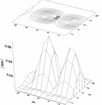
An amplitude (а) and argument (b) of approximate function are given in Figure 4 for c₁=1.6 and

2 1.2

c = . The amplitude values of the Fourier Transform coefficients corresponding to this solution are shown in

Figure 5. As we see in figure, the values of amplitudes of coefficients are nonsymmetrical concerning the plane

[image:9.595.100.245.495.673.2] [image:9.595.343.505.537.689.2]

(a)

[image:10.595.96.243.77.477.2]

(b)

Figure 4. The modulus (а) and argument (b) of approxima-tion funcapproxima-tion.

Figure 5. The optimum amplitude of Fouier transform coefficients.

YOZ, but the amplitude of approximate function (Figure 4,а) is symmetric.

For comparison of approximate functions, ponding to different solutions of (10), the curves corres-ponding to different types of the presented solutions in the section s₁≡0 are given in Figure 6. The curve 1 corresponds to the given function F(0,s2), the curve 2

– to branching-off solution, the curve 3 − to real solution

0(0, 2)

f s . Obviously that the branching-off solution bet-ter (in meaning of the functional σ) approaches the prescribed function by the module.

6. Conclusion

Mark the basic features and problems arising at investi-gation of the considered class of tasks:

The basic difficulty to solve this class of problems is study of nonuniqueness and branching of existing solu-tions dependent on the parameters c c₁, ₂ entering into the discrete Fourier Transform.

As follows from investigations, presented, in particu-lar, in [3,17] (for a special case, whenF s s( ,_{1 2})=

1( )1 2( )2

F s ⋅F s ), the quantity of the existing solutions grows considerably with increase of the parameters

1, 2

c c . Let us indicate, that in many practical applica-tions, in particular, in the synthesis problems of radiating systems, it is important to obtain the best approximation to the given function F s s( ,_{1 2}) at rather small values of parameters c c1, 2. This allows limiting by investigation

of several first points (lines) of branching.

To find the branching points (lines) of solutions of (8), it is necessary, as opposed to [3, 17], to solve not enough studied multiparametric spectral problem. The offered in this work approaches allow to find the solutions of a nonlinear two-parametric spectral problem for homoge-neous integral equations with degenerate kernels analyt-ically dependent on two spectral parameters.

0 0.2 0.4 0.6 0.81 1.2

-1 -0.5 030.512 1

| f |

s2

[image:10.595.90.255.521.691.2]

When finding the solutions to a system of Equation (14) by successive approximations method, to obtain the solutions of a certain type of parity of the function

(

1 2

)

arg f s s, it is necessary to choose an initial approxi-mation argf0

(

s s1, 2

)

of the same type of parity

ac-cording to (42).

To obtain the irrefragable answer concerning the branching-off solutions for certain values of parameters

1, 2

c c it is necessary to use the branching theory of so-lutions [18]. It is the object of special investigations.

7. References

[1] B. M. Minkovich and V. P. Jakovlev, “Theory of Synthesis of Antennas, ” Soviet Radio, Moscow, 1969.

[2] P. A. Savenko, “Numerical Solution of a Class of Nonlinear Problems in Synthesis of Radiating Systems,”Computational Mathematics and Mathematical Physics, Vol. 40, No. 6, 2000, pp. 889-899.

[3] P. O. Savenko, “Nonlinear Problems of Radiating Systems Synthesis (Theory and Methods of the Solution),” Institute for Applied Problems in Mechanics and Mathematics, Lviv, 2002.

[4] G. M. Vainikko, “Analysis of Discretized Methods,”Таrtus Gos. University of Tartu, Tartu, 1976.

[5] R. D. Gregorieff and H. Jeggle, “Approximation von Eigevwertproblemen bei nichtlinearer Parameterabhängi- keit,” Manuscript Math, Vol. 10, No. 3, 1973, pp. 245- 271.

[6] O. Karma, “Approximation in Eigenvalue Problems for Holomorphic Fredholm Operator Functions I,” Numerical Functional Analysis and Optimization, Vol. 17, No. 3-4, 1996, pp. 365-387.

[7] M. A. Aslanian and S. V. Kartyshev, “Updating of One Numerous Method of Solution of a Nonlinear Spectral Problem,”Journal of Computational Mathematics and Mathe- matical Physics, Vol.37, No. 5, 1998, pp. 713-717.

[8] S. I. Solov’yev, “Preconditioned Iterative Methods for a Class of Nonlinear Eigenvalue Problems,”Linear Algebra and its Applications, Vol. 41, No. 1, 2006, pp. 210-229.

[9] P. A. Savenko and L. P. Protsakh, “Implicit Function Method in Solving a Two-dimensional Nonlinear Spectral Problem,”

Russian Mathematics (Izv. VUZ), Vol. 51, No. 11, 2007, pp. 40-43.

[10] V. A. Trenogin, “Functional Analysis,” Nauka, Moscow ,1980. [11] I. I. Privalov, “Introduction to the Theory of Functions of

Complex Variables,” Nauka, Moscow, 1984.

[12] A. N. Kolmogorov and S. V. Fomin, “Elements of Functions Theory and Functional Analysis,” Nauka, Moscow, 1968. [13] P. P. Zabreiko, А. I. Koshelev and М. А. Krasnoselskii,

“Integral Equations,” Nauka, Moscow, 1968.

[14] М. А. Krasnoselskii, G. М. Vainikko, and P. P. Zabreiko,

“Approximate Solution of Operational Equations,” Nauka, Moscow, 1969.

[15] I. I. Liashko, V. F. Yemelianow and A. K. Boyarchuk, “Bases of Classical and Modern Mathematical Analysis,” Vysshaya Shkola Publishres, Kyiv, 1988.

[16] E. Zeidler, “Nonlinear Functional Analysis and Its Appli- cations I: Fixed-Points Theorem,” Springer-Verlag, New York, Berlin, Heidelberg, Tokyo, 1985.

[17] P. A. Savenko, “Synthesis of Linear Antenna Arrays by Given Amplitude Directivity Pattern,” Izv. Vysch. uch. zaved. Radiophysics, Vol. 22, No. 12, 1979, pp. 1498-1504.

[18] М. M. Vainberg and V. А. Trenogin, “Theory of Branching of Solutions of Nonlinear Equations,”Nauka, Moscow, 1969. [19] V. V. Voyevodin and Y. J. Kuznetsov, “Matrices and Calcu-

lations,” Nauka,Moscow, 1984.

[20] A. Gursa, “Course of Mathematical Analysis, Vol. 1, Part 1,” Moscow-Leningrad, Gos. Technical Theory Izdat, 1933.