1
Disentangling the Influence of Knowledge on Attribute Non-Attendance.
Erlend Dancke Sandorf a*, Danny Campbellb and Nick Hanleyc
a* The Norwegian College of Fishery Science, Faculty of Biosciences, Fisheries and Economics, University of Tromsø – The Arctic University of Norway, NO 9037 Tromsø, Corresponding Author: [email protected] b Economics Division, University of Stirling, Stirling, FK9 4LA, United Kingdom, e-mail: [email protected] c Department of Geography and Sustainable Development, University of St. Andrews, St. Andrews, KY16 9AL, United Kingdom, email: [email protected]
Abstract:
We seek to disentangle the effect of knowledge about an environmental good on respondents’ propensity to ignore one or more attributes on the choice cards in a discrete choice experiment eliciting people’s preferences for increased protection of cold-water corals in Norway. We hypothesize that a respondent’s level of knowledge influences the degree to which she ignores attributes. Respondents participated in a quiz on cold-water coral prior to the valuation task and we use the result of the quiz as an ex-ante measure of their knowledge. Our results suggests that a high level of knowledge, measured by a high quiz score, is associated with higher probabilities of attendance to the three non-cost attributes, although this effect is only significant for one of them. A higher quiz score is also associated with a significantly lower probability of attending to the cost attribute. Furthermore, although being told your score has mixed directional effects on attribute non-attendance, it does not significantly affect the probability of attending to any of the attributes. Finally, allowing for attribute non-attendance leads to substantially lower conditional willingness-to-pay estimates. This highlights the importance of measuring how much people know about the goods over which they are choosing, and underlines that more research is needed to understand how information influences the degree to which respondents ignore attributes.
Keywords: Attribute Non-Attendance, Discrete Choice Experiment, Knowledge, Attribute Processing Strategies,
2
1. Introduction:In environmental economics, it is common to use stated preference methods to elicit people’s preferences for environmental goods. For some such goods, scientific knowledge is limited and public awareness is low. This lack of familiarity poses a problem for the use of stated preference in cost-benefit analysis of public policy choice, since it implies making policy recommendation based on the preferences of “uninformed” respondents. For goods such as biodiversity conservation, it is therefore necessary to provide information about the relevant aspects of the environmental good prior to the valuation task, and do so in a manner that is meaningful to respondents (Álvarez-Farizo and Hanley, 2006, MacMillan et al., 2006). In the following, we make a distinction between exogenous information leading to objective knowledge, e.g. provided by the survey instrument, and endogenous information leading to subjective knowledge, e.g. gained through experience (Cameron and Englin, 1997). Information from both sources determines a respondent’s knowledge about the environmental good.
3
cards. As such, we investigate the connection between three important strands of the choice modeling literature.
The first concerns the effects of information and experience on stated preferences, an issue that has been of interest to practitioners since the first applications of contingent valuation to environmental goods. Early contributions to this literature are summarized in Munro and Hanley (2001). For example, Cameron and Englin (1997) found that experience with fishing significantly increased willingness-to-pay (WTP) for a doubling of the trout abundance in the North East United States. Recent studies have connected information and experience to how deterministic the choice process appears from an econometrician’s perspective. For example, Czajkowski et al. (2014a) find, in a stated preference study on biodiversity conservation management of Red Grouse in the UK uplands, that respondents receiving more complete and positive information have a more deterministic choice process, as seen from a practitioner’s perspective, but they observe only minor differences in WTP. In another study on the willingness-to-pay for beach water quality improvement among recreational beach users, Czajkowski et al. (2014b) find that as experience increase, preferences become more deterministic from a practitioners point of view, where experience is measured as number of days visiting the beach per year.
4
as text makes comparison of alternatives more difficult compared to a tabular presentation, and that the former leads to larger variance estimates and greater use of heuristics, in particular attribute elimination.
A related stream of research highlights the role of experience on being predisposed to different cognitive biases. For example, more experienced traders in a market for sports memorabilia were less prone to the endowment effect and likely to engage in more trades relative to inexperienced traders (List, 2003, List, 2011). Similarly, Feng and Seasholes (2005) found that experienced stock traders are less likely to suffer from the disposition effect, which is a reluctance to realize losses and an eagerness to realize gains. In other words, keeping a losing stock too long and selling a winning one too quickly. Trader experience significantly reduced loss sensitivity, but had limited effect on gains. A study of NY cab drivers show that experienced drivers work more on days where the earning potential is higher and less on days when it is worse, suggesting that these drivers are less prone to the bias of fixed working hours (Camerer et al., 1997).
The third relevant strand of the literature is that concerned with the nature of the utility function and whether people are indeed willing to make trade-offs between all attributes which are used to describe their choices (Colombo et al., 2013). Several papers within the stated preference literature have considered the implications of lexicographic preferences, where individual refuse to accept any increase in one desirable attribute to compensate for a decrease in a second desirable attribute (Rekola, 2003). Or, individuals may only be willing to make trade-offs between a pair of desirable attributes within certain ranges of values for these attributes – the cut-offs model (Bush et al., 2009). If the individual is unwilling to accept trade-offs (if they have “non-compensatory” preferences), then this may manifest as an unwillingness to pay attention to these attributes.
5
corals. We can thus explore how knowing how well or how badly you did on the quiz influences the likelihood of being predicted to have attended to or to have ignored an attribute.
Our results suggest a link between knowledge and attribute non-attendance. We find that scoring above the average in the cold water coral quiz is associated with a higher probability of attending to three environmental and ecological attributes of cold water coral conservation, although the effect is only significant for one out of three. A higher quiz score also results in a significantly lower probability of attending to the Cost attribute. This result holds irrespective of whether a respondent was informed about her score. Furthermore, we find that being told your score causes mixed effects on attribute non-attendance: for three out of four attributes, knowing your score is linked to smaller differences in predicted probabilities of attendance between low- and high-scoring respondents, although this effect is insignificant. Finally, we find that allowing for attribute non-attendance leads to substantially lower willingness-to-pay estimates, a result which others have obtained.
2. Data
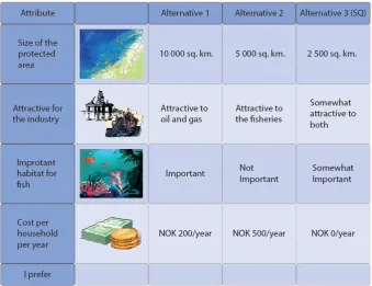
We use data from a discrete choice experiment (DCE) aimed at eliciting the Norwegian population’s preference for increased protection of cold-water coral off the coast of Norway (Aanesen et al., 2015). In the DCE we asked respondents to choose between two alternatives for increased cold-water coral protection and the situation today of only limited protection, which comes at zero additional cost. Each policy alternative was described by four attributes: the size of the protected area (Size), whether the area is important for the oil- and gas industries and/or commercial fisheries (Industry), whether the area is an important habitat for fish (Habitat), and the cost of each management scenario measured as a lump sum increase in annual national taxes (Cost). For example, the attribute Industry – Fisheries takes on the value of one if the area being protected is important for the fisheries. If true, then that means fishermen will have to relocate to other fishing grounds. As such, this attribute captures the likely impact of increased protection on industry. The Habitat attribute, on the other hand, takes on the value of one if the protected area is important habitat for fish and zero otherwise1. We show a sample choice card in Figure 1. The choice cards were constructed using a Bayesian efficient design where efficiency
6
was determined based on minimizing the d-error (Scarpa and Rose, 2008). The design was optimized for the multinomial logit model and updated based on two pilot studies to obtain more precise priors.
The data was gathered using a series of 24 valuation workshops in 22 municipalities in Norway in the spring of 2013. The selected municipalities are considered representative with regards to rural/urban and coastal/inland as well as general location within Norway. A professional survey company recruited participants to be representative with respect to age and gender in the chosen locations. Each valuation workshop consisted of between 12 and 23 participants. In total, usable responses from 397 participants were obtained. The main results and a detailed discussion of the data are found in Aanesen et al. (2015). This data has also been used by Sandorf et al. (2016) to compare valuation workshops with a probability based internet panel to assess the suitability of such panels to value complex and unfamiliar goods, and by La Riviere et al. (2014) to examine the effect of knowledge and objective signals on willingness-to-pay.
7
Figure 1 - Sample Choice Card (Translated into English)
3. Empirical Approach
In this section we describe the empirical approach and outline the discrete mixture random parameter logit model. We use a discrete mixture to probabilistically sort respondents into classes where attributes are either considered or ignored, and combine this with a random parameter logit model to uncover preference heterogeneity among respondents. We chose this approach for two reasons. First, it is computationally simpler (i.e. fewer estimated parameters) to estimate four probability functions, i.e. the probability of attending to each attribute as a function of the quiz score, and then construct a discrete mixing distribution as opposed to estimate separate probability functions for each class. Second, it makes the interpretation of the coefficients pertaining to hypothesis testing easier.
We test the following two hypotheses:
8
H2: being provided with an external signal about the extent of knowledge about the environmental good affects the attribute processing strategy adopted.
To introduce the notation we start by specifying a linear utility function that is separable in cost and other attributes. We assume that respondent i’s utility from choosing alternative j in choice situation t can be expressed as:
𝑈𝑖𝑗𝑡= 𝛽′𝑥𝑖𝑗𝑡+ 𝜀𝑖𝑗𝑡, (1)
where 𝛽 is a vector of parameters to be estimated, 𝑥𝑖𝑗𝑡 are the levels of the attributes and 𝜀𝑖𝑗𝑡 is an i.i.d. type I
extreme value distributed error term with constant variance π2/6. Given these assumptions, the probability of the sequence of choices made by respondent i is given by the multinomial logit model in Equation 2.
Pr(𝑦𝑖|𝑥𝑖) = ∏
exp (𝛽′𝑥𝑖𝑗𝑡) ∑𝑄 exp (𝛽′𝑥𝑖𝑞𝑡)
𝑞=1
𝑇
𝑡=1 , (2)
where 𝑦𝑖= < 𝑗𝑖1, 𝑗𝑖2, … , 𝑗𝑖𝑇 > and Q is the total number of alternatives.
Respondents may use a number of different attribute processing strategies, but in this paper, we focus on one: attribute non-attendance. For simplicity, we assume that an attribute is either fully attended to or not, rather than including cases where people only partly attend to an attribute (Erdem et al., 2015, Colombo et al., 2013). With four attributes, we end up with 24=16 possible combinations of attributes being attended to or not, i.e. 16 AN-A classes. We consider AN-A by assuming that we can probabilistically classify each respondent into one of the sixteen classes, where each class corresponds to one combination of attending to or ignoring attributes. Instead of specifying and estimating the probabilistic membership for each of the sixteen classes independently, we use a discrete mixture modelling framework. In a discrete mixture model, the parameters can only take on a finite number of values (see e.g. Hess et al., 2007, Hole, 2011). In our case, we use this to estimate the share of respondents who attend to or ignore each attribute. The (unconditional) probability that respondent i attends to attribute k is denoted by 𝜋𝑖𝑘1, and we estimate separate probabilities for each subgroup (defined on the basis
9
probability that respondent i ignores the attribute k, denoted by 𝜋𝑖𝑘0, is therefore 𝜋𝑖𝑘0 = 1 − 𝜋𝑖𝑘1. Next, we use
these probabilities to define the discrete mixing distribution. Let 𝑠 = 1, … , 𝑆 be an index over all possible combinations of the probabilities 𝜋𝑖𝑘1 and 𝜋𝑖𝑘0, which represents the discrete mixing distribution.
𝑆 =
{
𝑠 = 1 → 𝜔𝑖1= 𝜋𝑖 size0 × 𝜋𝑖 industry0 × 𝜋𝑖 habitat0 × 𝜋𝑖 cost0
𝑠 = 2 → 𝜔𝑖2= 𝜋𝑖 size0 × 𝜋𝑖 industry0 × 𝜋𝑖 habitat0 × 𝜋𝑖 cost1
𝑠 = 3 → 𝜔𝑖2= 𝜋𝑖 size0 × 𝜋𝑖 industry0 × 𝜋𝑖 habitat1 × 𝜋𝑖 cost0
𝑠 = 4 → 𝜔𝑖3= 𝜋𝑖 size0 × 𝜋𝑖 industry0 × 𝜋𝑖 habitat1 × 𝜋𝑖 cost1
⋮
𝑠 = 16 → 𝜔𝑖16= 𝜋𝑖 size1 × 𝜋𝑖 industry1 × 𝜋𝑖 habitat1 × 𝜋𝑖 cost1
(3)
We consider attribute non-attendance by restricting the parameter on the ignored attribute to zero in the likelihood function (Hensher et al., 2005). We accommodate this by introducing a vector of dummy variables,
𝛿𝑠, that take on the value zero for classes in which the corresponding value of 𝜋𝑖𝑘0 is used to determine the class
probability, 𝜔𝑖𝑠, and one otherwise.
Pr(𝑦𝑖|𝑥𝑖, 𝜔𝑖) = ∑𝑆𝑠=1𝜔𝑖𝑠 ∏
exp (𝛿𝑠𝛽′𝑥𝑖𝑗𝑡)
∑𝑄𝑞=1exp (𝛿𝑠𝛽′𝑥𝑖𝑞𝑡) 𝑇
𝑡=1 (4)
So far, we have assumed that all respondents (who consider the attributes) have the same marginal utilities. However, this is unlikely to be the case. For this reason, we allow for heterogeneous preferences, i.e. different marginal utilities of attributes across respondents, by allowing for random variations in the parameters. Let Θ represent the vector of random parameters and Ω denote the mean and variance of these parameter distributions, then we can denote the joint density of the parameters 𝛽 by 𝑓(Θ|Ω). The unconditional probability becomes the weighted integral over the logit formula over all possible values of the parameters as seen in Equation 5.
Pr(𝑦𝑖|𝑥𝑖, 𝜔𝑖, Ω) = ∑𝑆𝑠=1𝜔𝑖𝑠 ∫ ∏
exp (𝛿𝑠𝛽′𝑥𝑖𝑗𝑡)
∑𝑄𝑞=1exp (𝛿𝑠𝛽′𝑥𝑖𝑞𝑡)
𝑇
10
This integral does not have an analytical solution, but is approximated through simulation. Thus, our model represents a combination of a discrete and a continuous mixing model. Such models have previously been applied by e.g. Hole (2011), Doherty et al. (2013), Campbell and Doherty (2013) and Campbell et al. (2014).
Finally, we can obtain the conditional (i.e. individual specific) class membership probabilities (Equation 6) and conditional willingness-to-pay estimates (Equation 7) using Bayes’ theorem as follows (see e.g. Train, 2009):
𝜔𝑠|𝑖=∑ 𝜔𝑖𝑠𝜔Pr (𝑦𝑖|𝑥𝑖,𝜔𝑖,Ω)
𝑖𝑠 𝑆
𝑠=1 Pr (𝑦𝑖|𝑥𝑖,𝜔𝑖,Ω) (6)
wtp̂𝑖= ∑ 𝜔𝑠|𝑖∫ 𝜈 Pr(𝑦∫ Pr(𝑦𝑖|𝑥𝑖,𝜔𝑖,Ω)𝑓(Θ|Ω)𝑑(Θ)
𝑖|𝑥𝑖,𝜔𝑖,Ω)𝑓(Θ|Ω)𝑑(Θ)
𝑆
𝑠=1 (7)
where 𝜐 = −𝛽/𝛽cost. Notice that we weight the estimates by the conditional probability of being in a particular
class. It is important to stress that when we calculate willingness-to-pay from an attribute non-attendance model, we only include classes in which both the non-cost and cost attributes are considered. In the case where either is ignored, willingness-to-pay is undefined. The mean of a conditional distribution gives an indication as to where a given respondent is most likely to lie on the willingness-to-pay distribution (Hess, 2010).
4. Results:
4.1. Sample Description and Quiz Responses
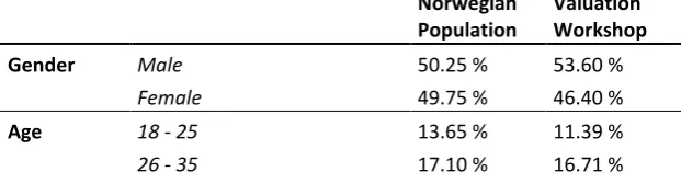
[image:10.595.72.383.682.771.2]Participants in the valuation workshop were sampled to be representative with respect to age and gender within the geographic locations. Looking at the composition of the sample (Table 1), we see that in terms of these characteristics, the sample matches the Norwegian population fairly well, albeit is skewed towards more educated and higher income individuals.
Table 1 - Demographic Composition of the sample
Norwegian Population
Valuation Workshop
Gender Male 50.25 % 53.60 %
Female 49.75 % 46.40 %
Age 18 - 25 13.65 % 11.39 %
11
36 - 45 18.26 % 19.49 %
46 - 55 17.22 % 19.75 %
56 - 65 14.80 % 14.43 %
66+ 18.98 % 18.23 %
Geographic Oslo and Akershus 23.69 % 20.40 % location Hedemark and Oppland 7.48 % 8.31 %
South-East Norway 18.98 % 14.36 % Agder and Rogaland 14.72 % 14.61 %
Western - Norway 17.14 % 19.40 %
Trøndelag 8.64 % 9.57 %
Northern Norway 9.36 % 13.35 %
Education Middle School or less 27.90 % 6.85 %
3 year high school 41.70 % 35.79 %
More than high school 30.40 % 57.36 % Personal Less than NOK 200.000 25.26 % 16.24 % Income 200.000 - 300.000 17.49 % 16.75 %
301.000 - 400.000 18.01 % 22.68 %
401.000 - 500.000 15.31 % 20.88 %
501.000 - 600.000 9.11 % 10.31 %
601.000 - 700.000 5.02 % 5.93 %
701.000 - 800.000 2.99 % 2.32 %
801.000 - 900.000 1.91 % 1.80 %
901.000 - 1.000.000 1.28 % 1.29 %
More than NOK 1.000.000 3.62 % 1.80 %
[image:11.595.72.383.77.437.2] [image:11.595.71.509.678.727.2]The maximum attainable quiz score was eight correct answers. We show the distribution of the quiz scores in Table 22. The mean score is 6.5 and the median score is seven correct answers. This means that 56 percent scored above the mean, i.e. median or higher. Approximately half of the sample were told their score prior to completing the valuation tasks. Interacting the dummies indicating score and treatment, we get four groups of roughly the same size: 27 percent scored above the mean and were told their score, 22 percent scored below the mean and were told their score, 29 percent scored above the mean and were not told their score and 22 percent scored below the mean and were not told their score.
Table 2 - Distribution of quiz scores
Distribution of respondents by quiz score
Score 1 2 3 4 5 6 7 8
Percent 0.00 % 1.50 % 1.80 % 3.30 % 12.90 % 24.50 % 27.50 % 28.50 %
12
Before we continue with the results of the estimation it is prudent to draw some comparisons to the paper by La Riviere et al. (2014) who use the same data, quiz and treatment. They investigate how knowledge about a good affects WTP and scale, and furthermore how an objective signal (receive one’s score) causes changes in WTP and scale. Using a heteroskedastic multinomial logit model they find that higher knowledge is associated with a more consistent choice process, but that receiving an objective signal had no significant impact. Using a multinomial logit model with interaction effects they find that scoring above the average and being told your score, significantly increase willingness-to-pay, although this result is driven by the Size attribute. While using the same data, the investigations in this paper departs from La Riviere et al. (2014) in one important way: We explore how knowledge about the good under consideration affects the probability of ignoring one or more attributes on the choice cards, and how receiving an external signal about your score cause changes in this probability. As such, we do not consider the same hypotheses as La Riviere et al. (2014).
4.2. Estimation results
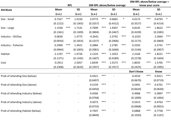
In order to test our hypotheses, we consider three models. Model 1 is a random parameters logit model, which serves as a reference for comparison and Model 2 and Model 3 are combinations of discrete and continuous mixture models to reveal attribute non-attendance and preference heterogeneity. In Model 2, we retrieve separate probabilities of attending to an attribute for respondents who scored below and above the average on the quiz. Model 3 is similar to Model 2, but with probabilities broken down for respondents who were and who were not told their quiz score. We report the unconditional probabilities of attendance to each attribute. We assume that the parameters on the non-Cost attributes follow a normal distribution and that the Cost parameter follows a lognormal distribution (with sign change). All three models are estimated using Ox version 7 (Doornik, 2007). Specifying the Cost parameter to follow a lognormal distribution implies that all respondents have a positive marginal utility of income and the willingness-to-pay distributions have defined moments (Daly et al., 2012). The models were estimated using 1000 scrambled Halton draws (Bhat, 2003). We report the results of the estimation in Table 33.
13
First, we look at the random parameters logit model (Model 1). In this model, we assume that a respondent attends to all the attributes. From Table 3, we see that the mean parameter estimates on the attributes Size, Industry – Fisheries and Habitat are significant at the one percent level, and that the mean parameter estimates on Industry – Oil/Gas and Cost are insignificant. Furthermore, a large increase in the protected area is preferred to a small increase. Results for the industry attribute are interesting. On average, whether an area is important for the oil- and gas industry does not influence utility, but if the area is important for fisheries, we have a positive influence on utility as such sites are designated for protection. One possible explanation is that during the presentation, respondents received information that the biggest threat to the cold-water coral reefs is bottom trawling. Protecting the area means reduced fishing pressure and hence reduced damage to the reefs. Furthermore, people have a strong preference for protecting an area that is important habitat for fish. The standard deviations of the parameter distributions are all highly significant for all attributes and, except for Habitat, larger than the corresponding mean values, indicating considerable preference heterogeneity.
14
Table 3 - Estimation results
Parameters of the Utility Functions
RPL DM-RPL above/below average
DM-RPL above/below average + know your score
Attribute Mean SD Mean SD Mean SD
(s.e.) (s.e.) (s.e.) (s.e.) (s.e.) (s.e.)
Size - Small 0.7327 *** 1.4150 3.9773 *** 0.6665 * 4.0173 *** 0.6793 *
(0.1222) (0.1363) (0.3257) (0.4312) (0.3527) (0.4214)
Size - Large 1.1558 *** 1.7141 4.7699 *** 1.9307 *** 4.8145 *** 1.8622 ***
(0.1361) (0.1309) (0.3804) (0.2467) (0.4109) (0.2385)
Industry - Oil/Gas 0.0630 1.3773 -0.2641 2.3742 *** -0.2325 2.2664 ***
(0.0934) (0.1053) (0.2237) (0.2906) (0.2175) (0.2869)
Industry - Fisheries 0.2969 *** 1.3421 0.2884 * 2.2785 *** 0.2593 2.2741 ***
(0.0964) (0.1005) (0.2081) (0.2668) (0.2146) (0.2907)
Habitat 2.1197 *** 1.9726 2.1224 *** 1.1023 *** 2.2164 *** 1.8221 ***
(0.1371) (0.1345) (0.1607) (0.4189) (0.2278) (0.1604)
Cost -0.2911 2.5057 1.8439 *** 1.5573 *** 1.8033 *** 1.5705 ***
(0.2308) (0.2633) (0.1937) (0.1917) (0.2425) (0.1995)
Don't Know Know
Prob of attending Size (below) - - 0.4321 *** - 0.4310 *** 0.4411 ***
(0.0497) (0.0670) (0.0719)
Prob of attending Size (above) - - 0.5159 *** - 0.5491 *** 0.4761 ***
(0.0450) (0.0620) (0.0630)
Prob of attending Industry (below) - - 0.4266 *** - 0.4968 *** 0.3897 ***
(0.0768) (0.1009) (0.1064)
Prob of attending Industry (above) - - 0.5073 *** - 0.5413 *** 0.4763 ***
(0.0733) (0.0968) (0.0952)
Prob of attending Habitat (below) - - 0.7507 *** - 0.6868 *** 0.7758 ***
15
Prob of attending Habitat (above) - - 1.0000 *** - 0.9813 *** 0.9503 ***
(0.0783) (0.0916) (0.0941)
Prob of attending Cost (below) - - 0.6329 *** - 0.6716 *** 0.6060 ***
(0.0633) (0.0866) (0.0830)
Prob of attending Cost (above) - - 0.4724 *** - 0.4945 *** 0.4659 ***
(0.0543) (0.0738) (0.0737)
Model Characteristics
Adj. Pseudo R - Squared 0.333 0.356 0.354
LL(0) -5144.8 -5144.8 -5144.8
Log Likelihood value -3417.6 -3295.5 -3295.1
AIC 6859.1 6631.1 6646.1
K 12 20 28
N 4683 4683 4683
*** Significant at the 1 % level
** Significant at the 5 % level
16
In Model 2, we test whether attribute non-attendance differs between low- and high knowledge individuals. We estimate the (unconditional) probabilities of attending to each of the attributes as a function of whether a given respondent scored above the average on the quiz4, and consider attribute non-attendance by restricting the parameter on the ignored attribute to zero in the likelihood function in the class in which the attribute was assumed ignored (Hensher et al., 2005). From Table 3, we see that the mean parameter estimates on Size, Habitat and Cost are significant at the one percent level, the estimate on Industry – Oil/Gas is significant at the ten percent level and the estimate on Industry – Fisheries is insignificant. The unconditional probabilities provides clear evidence that a large share of the sample did not consider all attributes. Importantly, we draw attention to the fact that considering AN-A has a bearing on the means and standard deviations uncovered for the attributes. In particular, we see that the Cost attribute is now highly significant (note that the parameters relate to the underlying Normal distribution). Moreover, while evidence of substantial preference heterogeneity among respondents remains, we now find that the standard deviations are relatively smaller compared to their respective means for all attributes, except for Industry. Crucially, this gives a clear signal that the preference heterogeneity retrieved in the naïve model is confounded with non-attendance. This is consistent with Hess et al. (2013), and further highlights the need to disentangle preference and processing heterogeneity.
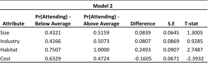
A comparison of the retrieved (unconditional) probabilities of attending to the attributes for respondents scoring below and above the average on the quiz (i.e., low and high levels of knowledge) reveals an interesting finding. For all non-Cost attributes we see a higher incidence of attribute non-attendance among respondents whose quiz score was below average. However, we find the reverse pattern for the Cost attribute—high scoring respondents are less likely to attend to Cost (recall that the quiz did not cover issues over costs). To further shed light on the issue and to corroborate our first hypothesis, in Table 4, we present test statistics of the differences in unconditional probabilities of attribute attendance. From this, we can see that the differences in rates of attendance between the two subgroups are only statistically significant for the Habitat and Cost attributes.
17
Table 4 - Testing for difference in (unconditional) probabilities of attendance
Model 2
Attribute
Pr(Attending) - Below Average
Pr(Attending) -
Above Average Difference S.E T-stat
Size 0.4321 0.5159 0.0839 0.0645 1.3005
Industry 0.4266 0.5073 0.0807 0.0869 0.9285
Habitat 0.7507 1.0000 0.2493 0.0907 2.7487
Cost 0.6329 0.4724 -0.1605 0.0671 -2.3932
18
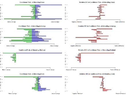
Figure 2- Conditional Probabilities of Attendance (Model 2)
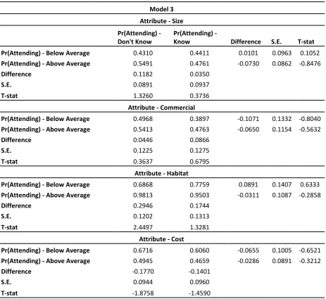
In Model 3, we test how receiving an external signal about the extent of knowledge about the environmental good affects the probability of attending to the attributes. We uncover different probabilities of attending to each of the attributes based on whether a respondent scored below or above the average and were and were not informed of their score. From Table 3, we notice that the estimated distributions of preferences in the sample are very similar to those obtained in Model 2, with a marginal improvement in model fit. However, the AIC statistic and pseudo R-squared, suggests that the model is less parsimonious. Still, we find evidence of preference heterogeneity as evident by the significant standard deviations.
19
[image:19.595.74.538.263.688.2]for respondents who did not know their score (Table 5). We observe a mixed directional effect in the probability of attendance between respondents scoring below the mean and were/were not told their score and scoring above the mean and were/were not told their score, although none of these differences are significant. This suggests that being told your score does not affect attribute non-attendance rates. A final observation, except for the Industry attribute, the difference in the probability of attendance between low- and high-scoring respondents is smaller, in absolute terms, for respondents who were told their score.
Table 5 - Testing for difference in (unconditional) probabilities of attendance
Model 3
Attribute - Size
Pr(Attending) - Don't Know
Pr(Attending) -
Know Difference S.E. T-stat Pr(Attending) - Below Average 0.4310 0.4411 0.0101 0.0963 0.1052 Pr(Attending) - Above Average 0.5491 0.4761 -0.0730 0.0862 -0.8476
Difference 0.1182 0.0350
S.E. 0.0891 0.0937
T-stat 1.3260 0.3736
Attribute - Commercial
Pr(Attending) - Below Average 0.4968 0.3897 -0.1071 0.1332 -0.8040 Pr(Attending) - Above Average 0.5413 0.4763 -0.0650 0.1154 -0.5632
Difference 0.0446 0.0866
S.E. 0.1225 0.1275
T-stat 0.3637 0.6795
Attribute - Habitat
Pr(Attending) - Below Average 0.6868 0.7759 0.0891 0.1407 0.6333 Pr(Attending) - Above Average 0.9813 0.9503 -0.0311 0.1087 -0.2858
Difference 0.2946 0.1744
S.E. 0.1202 0.1313
T-stat 2.4497 1.3281
Attribute - Cost
Pr(Attending) - Below Average 0.6716 0.6060 -0.0655 0.1005 -0.6521 Pr(Attending) - Above Average 0.4945 0.4659 -0.0286 0.0891 -0.3212
Difference -0.1770 -0.1401
S.E. 0.0944 0.0960
20
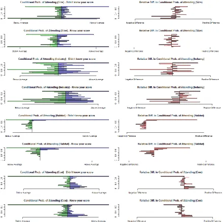
[image:20.595.77.518.271.709.2]A visual inspection of the conditional probabilities of attendance provides additional insight. For the Size attribute, we see that scoring above the average and not knowing your score is associated with a higher probability of attendance, whereas knowing your score yields mixed results. For the Industry attribute, it seems that scoring above the average is associated with higher probability of attendance, but the results are mixed. Looking at the conditional probability of attending to the Habitat attribute, we see that scoring above the average is associated with a higher probability of attendance irrespective of whether or not the respondent knew, but that the relationship is stronger if they did. For the Cost attribute, we observe that the conditional probability of attendance is lower for high-scoring respondents irrespective of being told their score.
21
So far, our results show that scoring above the average in the cold water corals quiz is associated with a higher probability of attending to the non-cost attributes and a lower probability of attending to the Cost attribute, irrespective of being told your score, although this effect is only significant for the Habitat and Cost attributes. Receiving information about how well you did on the quiz causes mixed impacts on attribute non-attendance, but in general it reduces the difference between respondents scoring above and below the average on the quiz. While we provide exogenous information to respondents, which should translate into objective knowledge, the presentation of information and our measure of knowledge could influence results5. However, we took every measure to make sure that the presentation of information about cold-water coral was balanced and that the information about the discrete choice experiment gave equal weight to each of the attributes. The quiz was only concerned with knowledge about the ecosystem itself and as such was neutral with respect to the attributes used in the discrete choice experiment. Taking a closer look at the connection between our measure of knowledge and education we find that scoring above the average on the quiz is practically uncorrelated with university education (0.087). Furthermore, we ran a probit model with scoring above the average as the dependent variable and included several socio-economic indicators as the independent variables. The results show that university level education does not significantly influence scoring above the average on the quiz6. As such, our measure of knowledge should be independent of education level7.
The question still remains, why we observe that scoring above the average is associated with a lower probability of attending to the cost attribute. A few possibilities come to mind. First, respondents have firsthand experience with money and, as such, are familiar with it. It is possible that they understood the cost attribute better than they understood the environmental attributes. Consequently, variations in their knowledge of the good might influence the probability of attendance to the non-Cost attributes differently. Second, the fact that they receive information about cold-water coral might give the impression that these ecosystems are particularly important and that we need to protect them, even though we made every effort to provide balanced and objective
5 We thank a reviewer for pointing this out.
6 These results are available from the corresponding author upon request.
22
information. Thus, we observe the tendency that increased knowledge reduces the probability of attending to the cost attribute. Third, we know that a substantial share of our respondents have higher education. Although our measure of knowledge is independent of education, higher education is associated with higher income, and given diminishing marginal returns on income, money might be of less importance to high income respondents. Fourth, it is possible that it simply reflects a higher preference for cold-water coral protection for this group.
4.3. Willingness-to-pay
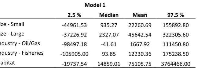
Here we report descriptive statistics of the means of the conditional (i.e. individual-specific) willingness-to-pay distributions. The mean of a conditional distribution gives an indication as to where a given respondent is most likely to lie on the willingness-to-pay distribution. We report the mean, median and 2.5 and 97.5 quantiles of the conditional willingness-to-pay distributions derived from Model 1, Model 2 and Model 3 in Table 6, Table 7 and Table 8, respectively. The willingness-to-pay estimates are conditional on the respondent’s choices, the distribution parameters and attribute levels and, importantly, on respondents considering both the non-Cost and Cost attributes. Note that in the case where the respondent ignored either the Cost or the non-Cost attribute, we have no information on the marginal utilities and consequently WTP is undefined.
Willingness-to-pay is reported in Norwegian Kroner (NOK) and at time of writing the exchange rate is € 1 = 8.63 NOK8. We see that the willingness-to-pay estimates from Model 1 are relatively high (Table 7)9. This high willingness-to-pay is possibly the result of attribute non-attendance and some respondents not considering cost. Furthermore, the lognormal distribution forces a large mass to be close to zero, a point that is underscored by the mean estimate on cost for the underlying normal distribution in Model 1 being insignificant, but becomes highly significant in Model 2 and Model 3 when attribute non-attendance is considered. From follow-up questions after the choice tasks, we know that 12 percent of respondents stated that the Cost attribute was not important when they made their choices between alternatives. Furthermore, the average conditional probability of being in a class where Cost was predicted to be ignored is 44.41 percent under the specification in Model 2
8 http://www.xe.com, 24-03-2015
23
[image:23.595.81.404.218.330.2]and 43.91 percent under the specification in Model 3. Not surprisingly, a large share of respondents is predicted to have extremely small marginal utility of money under Model 1. For this dataset, the implications of overlooking non-attendance of cost are clear to see, since we get very high willingness-to-pay estimates (because the denominator is very close to zero).
Table 6 - Willingness-to-pay estimates (Model 1)
Model 1
2.5 % Median Mean 97.5 %
Size - Small -44961.53 935.27 22260.69 155892.80 Size - Large -37226.92 2327.07 45642.54 322305.60 Industry - Oil/Gas -98497.18 -41.61 1667.92 111450.80 Industry - Fisheries -105905.00 93.85 12230.36 175238.50 Habitat -19737.54 14859.01 75105.75 3764466.00
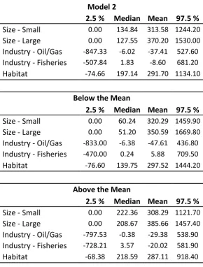
When we look at the willingness-to-pay derived from Model 2 (Table 7) and Model 3 (Table 8), we see that they are substantially lower, a result that is in line with the majority of studies looking at attribute non-attendance (see e.g. Colombo et al., 2013, Scarpa et al., 2013, Hensher et al., 2005, Campbell et al., 2008). Because we accommodate different class memberships, the conditional willingness-to-pay distributions differ for respondents above/below the median (Model 2) as well as for those being told/not being told their quiz score (Model 3). From the results in Table 7 we observe that scoring above the mean is associated with lower mean WTP, except for a large increase in the protected area and whether the protected area is important for the oil- and gas industry. From Table 8, when we also consider whether respondents received their score, we observe that scoring above the mean is associated with higher mean conditional WTP, except for industry-fisheries for treated individuals. In general, receiving your score is associated with lower mean conditional WTP for size-small and size-large irrespective of your score. Scoring below the mean and receiving your score is associated with higher mean conditional WTP for both the industry and habitat attributes. Scoring above the mean is associated with a slight increase in mean conditional WTP for industry-oil/gas, a slight decrease for industry-fisheries and marginal change in mean conditional WTP for habitat10.
24
Table 7 - Willingness-to-pay estimates (Model 2)
Model 2
2.5 % Median Mean 97.5 %
Size - Small
0.00
134.84 313.58 1244.20
Size - Large
0.00
127.55 370.20 1530.00
Industry - Oil/Gas
-847.33
-6.02
-37.41 527.60
Industry - Fisheries
-507.84
1.83
-8.60
681.20
Habitat
-74.66
197.14 291.70 1134.10
Below the Mean
2.5 % Median Mean 97.5 %
Size - Small
0.00
60.24
320.29 1459.90
Size - Large
0.00
51.20
350.59 1669.80
Industry - Oil/Gas
-833.00
-6.38
-47.61 436.80
Industry - Fisheries
-470.00
0.24
5.88
709.50
Habitat
-76.60
139.75 297.52 1444.20
Above the Mean
2.5 % Median Mean 97.5 %
Size - Small
0.00
222.36 308.29 1121.70
Size - Large
0.00
208.67 385.66 1457.40
Industry - Oil/Gas
-797.53
-0.38
-29.38 538.90
Industry - Fisheries
-728.21
3.57
-20.02 581.90
25
Table 8 - Willingness-to-pay estimates (Model 3)
Model 3
2.5 % Median Mean 97.5 %
Size - Small
0.00
131.26 313.05 1161.00
Size - Large
0.00
116.37 380.20 1535.50
Industry - Oil/Gas
-728.20
-6.08
-17.35 517.90
Industry - Fisheries
-522.20
-1.11
3.99
545.00
Habitat
-127.80
196.02 292.88 1198.20
Below the Mean - Don't know
Below the Mean - Told
2.5 % Median Mean 97.5 %
2.5 %
Median Mean
97.5 %
Size - Small
0.00
59.59
329.64 1704.10
Size - Small
0.00
70.24
258.45
950.30
Size - Large
0.00
56.13
376.19 1830.50
Size - Large
0.00
44.92
309.43
1402.80
Industry - Oil/Gas
-814.10
-6.89
-40.23 534.40
Industry - Oil/Gas
-480.10
-6.26
-34.62
262.20
Industry - Fisheries
-567.00
-3.47
8.38
534.30
Industry - Fisheries
-320.40
-2.44
10.18
318.60
Habitat
-144.50
111.64 279.72 1186.60
Habitat
-114.60
115.86
294.85
1595.20
Above the Mean - Don't know
Above the Mean - Treatment
2.5 % Median Mean 97.5 %
2.5 %
Median Mean
97.5 %
Size - Small
0.00
318.02 368.97 1102.80
Size - Small
0.00
141.27
283.04
1056.30
Size - Large
0.00
343.99 452.56 1440.10
Size - Large
0.00
111.26
362.64
1553.50
Industry - Oil/Gas
-734.10
-2.85
-13.85 529.10
Industry - Oil/Gas
-509.87
-2.80
11.78
519.90
Industry - Fisheries
-519.00
-3.94
9.18
673.30
Industry - Fisheries
-614.00
3.68
-10.23
430.20
26
5. Conclusion:We set out to disentangle the effect of knowledge about an environmental good on attribute non-attendance, using data from a discrete choice experiment on cold-water coral protection in Norway. Specifically we tested two hypotheses. First, that the probability of attending to an attribute differs between the low- and high-knowledge groups, and second, that being provided with an external signal about the extent of high-knowledge about the environmental good affects the probability of attendance. We undertook these tests by estimating a combination of discrete and continuous mixture models, where we probabilistically classified respondents into 16 classes, each describing one combination of attending to or ignoring a particular attribute.
Four attributes described each alternative in the discrete choice experiment: The size of the area, the importance of the area for two different industries, the importance of the area as habitat for marine life and the cost of the management scenario. Our results indicate that there is a link between knowledge and attendance (non-attendance). We observe that scoring above the average on the quiz, a measure of high knowledge, is associated with an increase in the predicted probability of attending to the Size, Industry and Habitat attributes, and a decrease in the predicted probability of attending to the Cost attribute. The difference in predicted probability of attendance is significant for the Habitat and Cost attribute.
27
In our dataset, we find that attribute non-attendance is prevalent and that failing to consider this leads to rather high willingness-to-pay estimates. We consider it important to be aware of respondents’ propensity to ignore attributes because it might lead the researcher to draw the wrong conclusion regarding respondents’ willingness-to-pay.
This paper shows that knowledge about the environmental good may influence a respondent’s propensity to ignore attributes on the choice cards and use a simplifying choice heuristic. A higher level of knowledge regarding the good significantly affected the probability of attending to two out of four attributes, but in different directions. Our results imply that choice modelling practitioners should be aware that information provided prior to the discrete choice experiment increases knowledge, which could affect the degree to which attributes are ignored. More research is needed to fully understand a priori what type of information affects attendance and in which direction. Understanding this is crucial to reduce attribute non-attendance and obtain more precise willingness-to-pay estimates.
Acknowledgements:
The data from the cold-water coral survey was collected as part of the project “Habitat-Fisheries interactions – Valuation and Bio-Economic Modeling of Cold-Water Coral”, funded by the Norwegian Research Council (grant no 216485). We thank Margrethe Aanesen for input, and Mikolaj Czajkowski and Jacob LaRiviere for major inputs to survey design. In addition, we thank two referees for helpful comments on an earlier version. We also thank the Marine Alliance Science and Tehcnology (MASTS: www.masts.ac.uk) for part funding this research. Any remaining errors are the sole responsibility of the authors.
References:
28
ALEMU, M. H., MØRKBAK, M. R., OLSEN, S. B. & JENSEN, C. L. 2013. Attending to the reasons for
attribute non-attendance in choice experiments. Environmental and resource economics,
1-27.
ÁLVAREZ-FARIZO, B. & HANLEY, N. 2006. Improving the process of valuing non-market benefits:
combining citizens’ juries with choice modelling. Land economics, 82, 465-478.
ALVAREZ-FARIZO, B., HANLEY, N., BARBERAN, R. & LAZARO, A. 2007. Choice modeling at the “market
stall”: Individual versus collective interest in environmental valuation. Ecological economics,
60, 743-751.
BHAT, C. R. 2003. Simulation estimation of mixed discrete choice models using randomized and
scrambled Halton sequences. Transportation Research Part B: Methodological, 37, 837-855.
BLAMEY, R. K., BENNETT, J. W., LOUVIERE, J. J., MORRISON, M. D. & ROLFE, J. C. 2002. Attribute
causality in environmental choice modelling. Environmental and Resource Economics, 23,
167-186.
BUSH, G., COLOMBO, S. & HANLEY, N. 2009. Should all choices count? Using the cut-offs approach to
edit responses in a choice experiment. Environmental and Resource Economics, 44, 397-414.
CAMERER, C., BABCOCK, L., LOEWENSTEIN, G. & THALER, R. 1997. Labor supply of New York City
cabdrivers: One day at a time. The Quarterly Journal of Economics, 407-441.
CAMERON, T. A. & ENGLIN, J. 1997. Respondent experience and contingent valuation of
environmental goods. Journal of Environmental Economics and Management, 33, 296-313.
CAMPBELL, D. & DOHERTY, E. 2013. Combining discrete and continuous mixing distributions to identify
niche markets for food. European Review of Agricultural Economics, 40, 287-312.
CAMPBELL, D., HENSHER, D. A. & SCARPA, R. 2011. Non-attendance to attributes in environmental
choice analysis: a latent class specification. Journal of environmental planning and
management, 54, 1061-1076.
CAMPBELL, D., HENSHER, D. A. & SCARPA, R. 2014. Bounding WTP distributions to reflect the
‘actual’consideration set. Journal of choice modelling, 11, 4-15.
CAMPBELL, D., HUTCHINSON, W. G. & SCARPA, R. 2008. Incorporating discontinuous preferences into
the analysis of discrete choice experiments. Environmental and resource economics, 41,
401-417.
CARLSSON, F., KATARIA, M. & LAMPI, E. 2010. Dealing with ignored attributes in choice experiments
on valuation of Sweden’s environmental quality objectives. Environmental and resource
economics, 47, 65-89.
C
CAUSSADE, S., ORTÚZAR, J. D. D., RIZZI, L. I. & HENSHER, D. A. 2005. Assessing the influence of design
dimensions on stated choice experiment estimates. Transportation research part B:
Methodological, 39, 621-640.
COLOMBO, S., CHRISTIE, M. & HANLEY, N. 2013. What are the consequences of ignoring attributes in
choice experiments? Implications for ecosystem service valuation. Ecological Economics, 96,
25-35.
CZAJKOWSKI, M., HANLEY, N. & LARIVIERE, J. 2014a. Controlling for the effects of information in a
public goods discrete choice model. Environmental and Resource Economics, 1-22.
CZAJKOWSKI, M., HANLEY, N. & LARIVIERE, J. 2014b. The effects of experience on preferences: theory
and empirics for environmental public goods. American Journal of Agricultural Economics,
aau087.
DALY, A., HESS, S. & TRAIN, K. 2012. Assuring finite moments for willingness to pay in random
coefficient models. Transportation, 39, 19-31.
DOHERTY, E., CAMPBELL, D., HYNES, S. & VAN RENSBURG, T. M. 2013. Examining labelling effects
within discrete choice experiments: An application to recreational site choice. Journal of
environmental management, 125, 94-104.
29
EDINGER, E. N., WAREHAM, V. E. & HAEDRICH, R. L. 2007. Patterns of groundfish diversity and
abundance in relation to deep-sea coral distributions in Newfoundland and Labrador waters.
Bulletin of Marine Science, 81, 101-122.
ERDEM, S., CAMPBELL, D. & HOLE, A. R. 2015. Accounting for Attribute‐Level Non‐Attendance in a
Health Choice Experiment: Does it Matter? Health economics, 24, 773-789.
FENG, L. & SEASHOLES, M. S. 2005. Do investor sophistication and trading experience eliminate
behavioral biases in financial markets? Review of Finance, 9, 305-351.
FOSSÅ, J., MORTENSEN, P. & FUREVIK, D. 2002. The deep-water coral Lophelia pertusa in Norwegian
waters: distribution and fishery impacts. Hydrobiologia, 471, 1-12.
FREIWALD, A., FOSSÅ, J. H., GREHAN, A., KOSLOW, T. & ROBERTS, J. M. 2004. Cold-water coral reefs.
UNEP-WCMC, Cambridge, UK, 84.
HENSHER, D. A. 2006. How do respondents process stated choice experiments? Attribute
consideration under varying information load. Journal of Applied Econometrics, 21, 861-878.
HENSHER, D. A., ROSE, J. & GREENE, W. H. 2005. The implications on willingness to pay of respondents
ignoring specific attributes. Transportation, 32, 203-222.
HESS, S. 2010. Conditional parameter estimates from Mixed Logit models: distributional assumptions
and a free software tool. Journal of Choice Modelling, 3, 134-152.
HESS, S., BIERLAIRE, M. & POLAK, J. W. 2007. A systematic comparison of continuous and discrete
mixture models. European Transport, 37, 35-61.
HESS, S., STATHOPOULOS, A., CAMPBELL, D., O’NEILL, V. & CAUSSADE, S. 2013. It’s not that I don’t
care, I just don’t care very much: confounding between attribute non-attendance and taste
heterogeneity. Transportation, 40, 583-607.
HOEHN, J. P., LUPI, F. & KAPLOWITZ, M. D. 2010. Stated choice experiments with complex ecosystem
changes: the effect of information formats on estimated variances and choice parameters.
Journal of Agricultural and Resource Economics, 568-590.
HOLE, A. R. 2011. A discrete choice model with endogenous attribute attendance. Economics Letters,
110, 203-205.
HOVLAND, M. & MORTENSEN, P. B. 1999. Norske korallrev og prosesser i havbunnen [Norwegian coral
reefs and processes in the ocean floor], Bergen, Norway, John Grieg Forlag.
HUSEBØ, Å., NØTTESTAD, L., FOSSÅ, J., FUREVIK, D. & JØRGENSEN, S. 2002. Distribution and
abundance of fish in deep-sea coral habitats. Hydrobiologia, 471, 91-99.
KOSENIUS, A.-K. 2013. Preference discontinuity in choice experiment: Determinants and implications.
The Journal of Socio-Economics.
LA RIVIERE, J., CZAJKOWSKI, M., HANLEY, N., AANESEN, M., FALK-PETERSEN, J. & TINCH, D. 2014. The
value of familiarity: Effects of knowledge and objective signals on willingness to pay for a
public good. Journal of Environmental Economics and Management, 68, 376-389.
LIST, J. A. 2003. Does market experience eliminate market anomalies? Quarterly Journal of Economics,
118, 41-72.
LIST, J. A. 2011. Does market experience eliminate market anomalies? The case of exogenous market
experience. American Economic Review, 101, 313-317.
MACMILLAN, D., HANLEY, N. & LIENHOOP, N. 2006. Contingent valuation: Environmental polling or
preference engine? Ecological economics, 60, 299-307.
MACMILLAN, D. C., PHILIP, L., HANLEY, N. & ALVAREZ-FARIZO, B. 2002. Valuing the non-market
benefits of wild goose conservation: a comparison of interview and group based approaches.
Ecological Economics, 43, 49-59.
MUNRO, A. & HANLEY, N. D. 2001. Information, uncertainty, and contingent valuation. In: BATEMAN,
I. J. & WILLIS, K. G. (eds.) Valuing Environmental Preferences: Theory and Practice of the
Contingent Valuation Method in the US, EU, and Developing Countries Oxford University Press,
Oxford.
30
SANDORF, E. D., AANESEN, M. & NAVRUD, S. 2016. Valuing unfamiliar and complex environmental
goods: A comparison of valuation workshops and internet panel surveys with videos.
Ecological Economics, 129, 50-61.
SCARPA, R., GILBRIDE, T. J., CAMPBELL, D. & HENSHER, D. A. 2009. Modelling attribute non-attendance
in choice experiments for rural landscape valuation. European Review of Agricultural
Economics, 36, 151-174.
SCARPA, R. & ROSE, J. M. 2008. Design efficiency for non‐market valuation with choice modelling: how
to measure it, what to report and why. Australian journal of agricultural and resource
economics, 52, 253-282.
SCARPA, R., ZANOLI, R., BRUSCHI, V. & NASPETTI, S. 2013. Inferred and stated attribute
non-attendance in food choice experiments. American Journal of Agricultural Economics, 95,
165-180.
STONE, R. 2006. Coral habitat in the Aleutian Islands of Alaska: depth distribution, fine-scale species
associations, and fisheries interactions. Coral reefs, 25, 229-238.
TRAIN, K. E. 2009. Discrete Choice Methods with Simulation, New York, Cambridge University Press.
Appendix A – A quiz on Cold-Water Corals (correct answer is underlined)
Q1: What is a coral?
1. An animal 2. A plant 3. A fungus 4. I do not know
Q2: At which depths do we find most cold-water corals?
1. < 30 meters 2. 30 – 100 meters 3. > 100 meters 4. I do not know
Q3: How much do cold-water corals grow annually?
31
Q4: What do cold-water corals eat?1. They emit secretions that attract fish that they catch and eat
2. They filter small organisms and suspended matter that happens to pass by 3. They photosynthesize with the help of a symbiotic algae
4. I do not know
Q5: What is the main threat to cold-water corals?
1. Predation by fish
2. Destruction by wave action 3. Bottom trawling
4. I do not know
Q6: At what temperature range do cold-water corals grow?
1. 0 °C – 4 °C 2. 4 °C – 13 °C 3. 13 °C – 18 °C 4. I do not know
Q7: How do cold-water corals reproduce?
1. Asexually through budding where a polyp divides into two genetically identical pieces 2. Sexually where a sperm fertilizes an egg that develops into a larva
3. Both sexually and asexually 4. I do not know
Q8: How old is the oldest cold-water coral reef found off the Norwegian coast?
1. Less than 1000 years old