Mixed effect models in distance sampling

(1)

-KMJBHF> 9>?MFJ> 6BABGKQBJ

, ;EBNFN 9P?IFOOBA CKM OEB .BDMBB KC 7E. >O OEB

<JFQBMNFOT KC 9O ,JAMBRN

&$%'

0PHH IBO>A>O> CKM OEFN FOBI FN >Q>FH>?HB FJ 8BNB>M@E+9O,JAMBRN*0PHH;BSO

>O*

EOOL*##MBNB>M@E!MBLKNFOKMT"NO!>JAMBRN">@"PG#

7HB>NB PNB OEFN FABJOFCFBM OK @FOB KM HFJG OK OEFN FOBI*

EOOL*##EAH"E>JAHB"JBO#%$$&'#'(%)

(2)

MIXED EFFECT MODELS IN DISTANCE SAMPLING

Cornelia Sabrina Oedekoven

Thesis submitted for the degree of DOCTOR OF PHILOSOPHY in the Schools of Mathematics and Statistics

UNIVERSITY OF ST ANDREWS ST ANDREWS

JANUARY 2013

c

(3)

(4)

(5)

Diese Arbeit ist meinen Eltern Herta und Peter Oedekoven gewidmet, von denen eine(r) das Talent hatte, Klassenbeste(r) im Statistikkurs an der Universität zu Köln zu sein, und der/die andere die Ausdauer, sich durch den selben Statistikkurs zu kämpfen, um weiterhin gemeinsam Kurse besuchen zu können.

This thesis is dedicated to my parents Herta and Peter Oedekoven, of whom one had the skills to be the best student in their statistics class at University of Cologne and one had the perseverance to struggle through the same statistics class so that they could continue their classes together.

Herta und Peter Oedekoven

(6)

Abstract

Recently, much effort has been expended for improving conventional distance

sam-pling methods, e.g. by replacing the design-based approach with a model-based

ap-proach where observed counts are related to environmental covariates (Hedley and

Buckland, 2004) or by incorporating covariates in the detection function model

(Mar-ques and Buckland, 2003).

While these models have generally been limited to include fixed effects, we propose

four different methods for analysing distance sampling data using mixed effects

mod-els. These include an extension of the two-stage approach (Buckland et al., 2009),

where we include site random effects in the second-stage count model to account for

correlated counts at the same sites. We also present two integrated approaches which

include site random effects in the count model. These approaches combine the

analy-sis stages for the detection and count models and allow simultaneous estimation of all

parameters. Furthermore, we develop a detection function model that incorporates

random effects.

We also propose a novel Bayesian approach to analysing distance sampling data which

(7)

tainty. Lastly, we propose using hierarchical centering as a novel technique for

improv-ing model miximprov-ing and hence facilitatimprov-ing an RJMCMC algorithm for mixed models.

We analyse two case studies, both large-scale point transect surveys, where the

in-terest lies in establishing the effects of conservation buffers on agricultural fields. For

each case study, we compare the results from one integrated approach to those from

the extended two-stage approach. We find that these may differ in parameter

es-timates for covariates that were both in the detection and the count model and in

model probabilities when model uncertainty was included in inference. The

perfor-mance of the random effects based detection function is assessed via simulation and

when heterogeneity in the data is present, one of the new estimators yields improved

results compared to conventional distance sampling estimators.

(8)

Acknowledgements

• Many thanks to my supervisors

I am most thankful to my supervisors Steve Buckland and Monique Macken-zie for fruitful discussions during out meetings, for being a great inspiration in terms of statistical methods and teaching, and, particularly to Steve, for amaz-ingly quick and kind revisions of the various chapter drafts with, oftentimes, same day returns.

• Many thanks to my colleagues within CREEM

Ruth King for her advice on Bayesian methods. Len Thomas for various dis-cussions on different statistical and ecological topics. Yuan Yuan for her help with the Latex text editor. Rhona Rodgers for her organisational skills. Phil Le Feuvre for his IT skills and rescuing me out of two hard drive meltdowns. The open door policy of all staff (including senior staff) at CREEM in general.

• Many thanks to my colleagues outside CREEM

Jeff Laake, NOAA, for his advice on chapter 6. David Miller, University of Rhode Island, for advice on variance estimation within program Distance. William Browne, University of Bristol, for his thoughts that inspired me to the methods from chapter 5. Kristine Evans and Loren W. Burger, Mississippi State University, for allowing me to use the indigo bunting and the covey data as case studies and Kristine for insights into the data collection process for both case studies.

• Many thanks to my friends at CREEM

Glenna Evans, Calum Brown, Danielle Harris, Yuan Yuan, Darren Kidney,

(9)

Data acknowledgements

The National CP-33 Monitoring Program was funded by the Multistate Conservation Grant Program (Grant MS M-1-T), which is supported by the Wildlife and Sport Fish Restoration Program and managed by the Association of Fish and Wildlife Agencies and US Fish and Wildlife Service. Further support was provided by the US Department of Agriculture (USDA) Farm Service Agency and USDA Natural Resources Conservation Service Conservation Effects Assessment Project. Collabo-rators included the AR Game and Fish Commission, GA Department of Natural Re-sources (DNR), IL DNR/Ballard Nature Center, IN DNR, IA DNR, KY Department of Fish and Wildlife Resources/KY Chapter of The Wildlife Society, MS Depart-ment of Wildlife, Fisheries and Parks, MO DepartDepart-ment of Conservation, NE Game and Parks Commission, NC Wildlife Resources Commission, OH DNR, SC DNR, TN Wildlife Resources Agency, TX Parks and Wildlife Department, Southeast Quail Study Group and Southeast Partners In Flight.

Institutional funding acknowledgements

For this PhD project I was supported by a studentship jointly funded by the University of St Andrews and EPSRC, through the National Centre for Statistical Ecology.

(10)

List of Figures

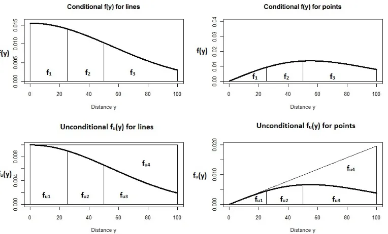
3.1 Examples for a conditional and unconditional likelihood with a

half-normal model using the same scale parameter (σ = 55) plotted between

0 and w = 100 including three distance intervals. The f1, f2, f3 and

fu1, fu2, fu3, fu4 refer to the cell probabilities. For the conditionalf(y) :

P3

i=1fi = 1, while for the unconditional fu(y) :P4i=1fui = 1. . . 37

6.1 Half-normal detection functions for which the scale parameter was

modelled with random effects. Shown are the functions resulting from

the minimum, maximum, 2.5 and 97.5 percentiles and the mean of

randomly sampled 200 coefficients be. In addition, the mean of all

detection functions is plotted in green. . . 118

(15)

2.1 Maximum likelihood estimates (MLE), analytic (ASE) and bootstrap

(BSE) standard errors for model parameters obtained by the two-stage

approach for best models. Shape parameters for the one-parameter

hazard-rate detection function were fixed. . . 25

2.2 Models and their probabilities resulting from bootstrap analysis. Each

count model included a fixed effect intercept and a random effect for

site in addition to shown covariates (JD = Julian day). Model

prob-abilities refer to the percentage of times the respective models were

chosen during 999 bootstrap iterations. . . 29

2.3 Maximum likelihood estimates (MLE), bootstrap standard errors (BSE)

and 95% confidence intervals (CI) using the two-stage approach for the

models with the highest probabilities (see Table 2.2 for model

proba-bilities). Units of measurements were metres for the detection function

model and square metres for the count model. . . 30

(16)

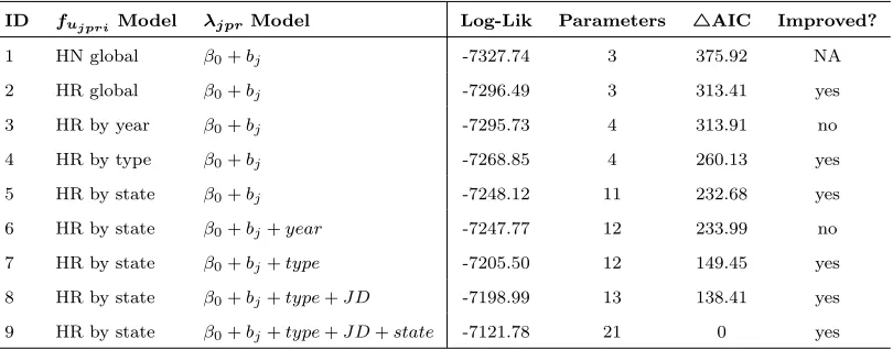
3.1 Models included in the forward stepwise model selection for the

inte-grated approach including the half-normal (HN) and the global and

stratified hazard-rate (HR) detection functions for fujpri and the

in-clusion of four covariates for λjpr in addition to the intercept β0 and

the random effects bj. 4AIC is given in relation to the overall best

model (model 9). Improved? refers to whether in this iterative model

selection process starting with model 1 the respective model yielded

an improved AIC compared to the previous and whether it should be

retained. . . 43

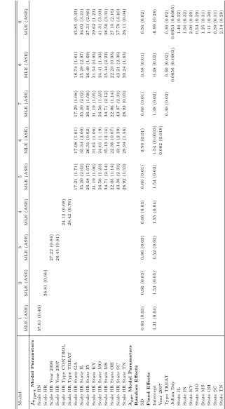
3.2 Maximum likelihood estimates (MLE) and analytical standard errors

(ASE) for parameters of contending models for the integrated approach

(models 1 through 9, Table 1). For the fujpri model, HN and HR refer

to the half-normal and hazard-rate detection functions respectively. . 45

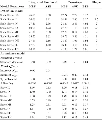
3.3 Maximum likelihood estimates (MLE), analytic (ASE) and bootstrap

(BSE, two-stage approach only) standard errors for model parameters

obtained by the integrated and the two-stage approach for best models.

Shape parameters for the one-parameter hazard-rate detection function

were fixed. . . 47

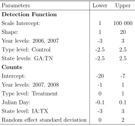
4.1 Lower and upper bounds for uniform prior distributions for all model

parameters. The different states included GA, IA, IL, IN, KY, MO,

MS, NC, SC, TN and TX. . . 67

(17)

the RJMCMC algorithm. All parameters were categorical, except for

continuous Julian day. . . 69

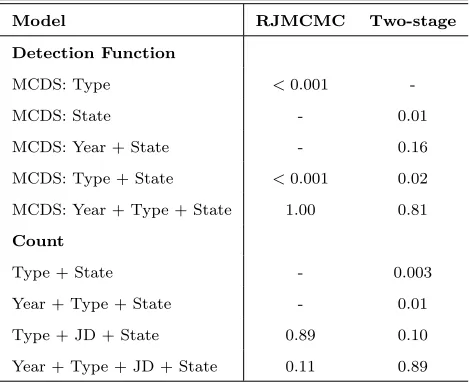
4.3 Models and their probabilities resulting from RJMCMC and bootstrap

analyses. Each count model included a fixed effect intercept and a

random effect for site in addition to shown covariates (JD = Julian

day). Model probabilities refer to the percentage of times the respective

models were chosen during 90 000 iterations (after 10 000 iterations of

burn-in) for RJMCMC and during 999 bootstrap iterations. . . 70

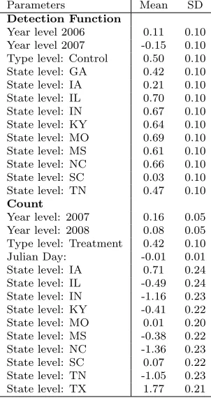
4.4 Mean, standard deviation (SD) and 95% credible intervals (CRI) from

the RJMCMC analysis along with maximum likelihood estimates (MLE),

bootstrap standard errors (BSE) and 95% confidence intervals (CI)

us-ing the two-stage approach for the models with the highest

probabil-ities (see Table 4.3 for model probabilprobabil-ities). Units of measurements

were metres for the detection function model and square metres for

the count model. . . 72

5.1 Means and standard deviations (SD) of normal proposal distributions

for model parameters as well as their lower and upper boundaries for

uniform prior distributions. HN and HR refer to the half-normal and

the hazard-rate detection functions respectively. . . 95

5.2 Posterior model probabilities for the analyses of the indigo bunting

data. GZM and the HC analyses did not include state in the initial

model. GZM-state and HC-state did include state in the initial model. 96

(18)

5.3 Mean and 95% credible intervals for models with highest posterior

support from the respective analyses. State level GA is absorbed in

the intercept. . . 98

5.4 Effective sample sizes for model parameters from the four RJMCMC

analyses. . . 100

6.1 Settings for the four sets of simulations: K and N respectively refer

to the total number of lines and animals in the study area, w is the

truncation distance, β0 and σb are the detection function parameters

and πa is the proportion of the study area covered. Also shown are

the resulting means (and standard deviations) of the total number of

detections, detections per line and lines with detections. Note that the

size of the study area A varied between sets with A = 2wK/πa. . . . 116

6.2 Mean (and standard deviation) of parameters estimates obtained from

1000 simulations using the half-normal detection function with and

without random effects (RE). . . 121

6.3 Average bias of abundance estimates (and standard errors) yielded by

different estimators. The estimators involving Pa did not include a

random effect in the detection function, those involving Pr did. . . . 122

6.4 Coverage rates of log-normal 95% confidence intervals around estimates

of abundance in the study area yielded by the different estimators. . . 123

6.5 Assessing performance of variance estimators by comparing the

stan-dard deviation of the 1000 abundance estimates (sd) to the mean of the

standard errors associated with the individual abundance estimates ( ¯se).124

(19)

ulations without random effects yielded by the estimators in the left

column. . . 125

(20)

Chapter 1 Introduction

1.1 Conventional distance sampling

Distance sampling is a tool for assessing wildlife abundance that is commonly used

when the interest lies in evaluating how many individuals (or clusters of individuals)

of the species of interest occur in a defined study area (e.g. Buckland et al., 2000;

Ca˜nadas and Hammond, 2006; Marques et al., 2007). Although the methods are also

applicable to plants (Buckland et al., 2007), we will generally speak of animals in the

following.

Distance sampling comprises a suite of methods, e.g. line transect sampling (e.g.

Burnham et al., 1980), point transect sampling (e.g. Buckland, 2006), cue counting

(e.g. Borchers et al., 2009) or trapping point transects (e.g. Buckland et al., 2006;

Potts et al., 2012). We focus on line or point transects in the following.

Tradition-ally, each of these methods requires that samplers such as lines or points are placed

within the study area according to some sampling design and that an observer makes

detections of the species of interest along or at these samplers.

(21)

These methods share an underlying concept which recognises that some of the animals

within the search area are not detected and that the proportion of those that were

missed can be estimated by collecting additional information. This additional

infor-mation usually consists of the distance to the detection, i.e. perpendicular distance

from the line for line transects or radial distance from the point for point transects

(Buckland et al., 2001).

These distances are used to estimate a detection function which models the decay

in detection probabilities with increasing distance from the sampler. This detection

function may then be used to estimate the average detection probability within the

search area, which is used to scale up the number of observed detections to an

esti-mate of the number of individuals in the search area (or number of clusters in the

case that detections are made of clusters of individuals). The latter is converted into

an estimate of abundance in the study area using a design-based approach where the

number of individuals in the search area is divided by the proportion of the study

area that was searched. Estimators of abundance or density of the study species are

summarised in Buckland et al. (2001). These conventional distance sampling (CDS)

methods rely on several assumptions (Buckland et al., 2001; Burnham et al., 1980):

I. All animals on the line or point are detected with certainty. If some animals on

the line are missed, due to perception or availability bias, resulting abundance

estimates are likely to be negatively biased.

II. Samplers are located according to a survey with an element of randomisation.

Meeting this assumption has two main consequences.

A: It insures that the area that was searched is a good representation of the

(22)

3

an encounter rate estimate in the search area to an encounter rate estimate in

the study area.

B: Placement of samplers in the study area is independent from the distribution

of animals. Estimators for the average detection probability in the search area

incorporate a function that describes the expected distribution of animals in the

search area with respect to increasing distance from the line or point. Using

CDS methods, we assume that this distribution is on average uniform for lines

and linearly increasing for points, which requires that this assumption is met.

III. Distances are measured without error. Measurement errors may lead to biased

abundance estimates by over- or underestimating the average detection

proba-bility.

IV. Observation process is a snapshot and animals are detected at their initial

lo-cation. For line and point transects, bias in the estimate of average detection

probability may arise due to animal movement whether the movement is random

or responsive to the observer.

V. Detections are independent.

In addition to these assumptions, reliable estimation of abundance using distance

sampling methods requires that:

i. The detection function is sufficiently flexible to capture the decay in detection

probability well and allow unbiased estimation of the average detection

probabil-ity - often referred to as the pooling robustness property. For CDS methods, a

(23)

from a suite of contending models including different key functions, possibly in

combination with adjustment terms (Buckland et al., 2001).

ii. The detection function has a ‘shoulder’, i.e. that animals out to some distance

from the line are detected with certainty - often referred to as the shape criterion.

iii. The number of samplers is large and that the samplers constitute a good

rep-resentation of the study area. This allows reliable scaling up from number of

animals in the search area to abundance in the study area. In addition, this

en-sures that the distribution of animals with respect to the samplers is on average

as described under assumption II.

iv. Samplers are independent from each other.

1.2 Recent developments in distance sampling

Over the past decade or so, a lot of effort has been invested into developing distance

sampling methods that allow one or more of these assumptions to be relaxed. With

reference to the above lists, these include:

I. Mark-recapture distance sampling

Borchers et al. (1998) developed mark-recapture distance sampling methods

(MRDS) for line transect surveys where detection on the line is not certain.

These authors combined mark-recapture and distance sampling methods where

two independent observers simultaneously conduct the transect survey and set

up mark-recapture trials for each other. This allows the number of animals

(24)

5

heterogeneity in the detection models and explored different levels of

indepen-dence between the two observers (e.g. Borchers et al., 2006; Buckland et al.,

2010). Laake et al. (2011) developed MRDS methods for point transects.

II. Modelling non-independent distribution of animals with respect to samplers

Marques et al. (2010) and Marques et al., in press, developed estimators that

replace the assumed distribution of animals with respect to increasing distance

from the samplers for CDS methods with a model of the estimated distribution of

animals with respect to the linear feature from which the survey was conducted.

III. Models for measurement errors in distance sampling

Borchers et al. (2010) developed estimators for a detection function for distance

data with systematic and with stochastic measurement errors. Marques (2004)

proposed estimators for density in the case of multiplicative errors in distance

measurements.

IV. Dealing with animal movement

Fewster et al. (2008) applied MRDS methods to double observer line transect

data to show that animal movement may constitute a problem for species of high

mobility. DiTraglia (2007) proposed adjusted line transect estimators which

in-corporate movement models. Buckland (2006) showed that for some songbirds,

point transects using the snapshot method may produce results with less bias.

Spear et al. (1992) and Spear and Ainley (1997a,b) proposed methods for

cor-recting abundance estimates for directionally flying seabirds obtained from strip

transects by taking into account the birds’ flight speed and direction in relation

(25)

V. Covariate models for observed counts at the samplers

Hedley and Buckland (2004) replaced the design-based approach from CDS with

a model-based approach using spatial models that relate animal density to

spa-tial and/or habitat covariates. These models may then be used to make

predic-tions on animal densities throughout the study area, including those parts that

were not surveyed. These methods do not require that the survey followed a

random design.

The two-stage approach (Buckland et al., 2009) may be used for those studies

where the interest lies in the relationship between animal densities and the

co-variates, e.g. for designed experiments where a treatment was applied to part of

the study area.

i. Increasing the flexibility of detection functions

Marques and Buckland (2003, 2004) increased the flexibility of detection functions

by modelling heterogeneity in detection probabilities between detected objects.

Their approach incorporates covariates affecting detection probabilities in the

scale parameter of the half-normal or hazard-rate detection function.

Miller and Thomas, unpublished manuscript, proposed using mixture models.

These are composed of two or more detection functions which are scaled using a

(26)

7

1.3 Developments of distance sampling methods

proposed in this thesis

While this list of developments in distance sampling methodology is far from

exhaus-tive, it demonstrates the need to supplement or replace some of the methods within

CDS. However, in most cases (with the exception of Potts (2011) and Yuan et al.,

unpublished manuscript) these approaches do not make use of random effects in their

models. The main objective of this thesis is to develop estimators, likelihood

formula-tions and algorithms for incorporating random effects, for which we generally assume

normality with a zero-mean and unknown standard deviation, into models applied to

distance sampling data. In particular, we address two main areas of incorporating

random effects: the covariate model for counts or densities on the plot (chapters 2 to

5) and the detection function model (chapter 6).

In chapter 2 we begin by describing an extended version of the two-stage approach

(Buckland et al., 2009) where we include random effects in the count model to

accom-modate correlated measurements, e.g. due to closeness of samplers in space or repeat

sampling at the same line or point. Hence, we present methods that do not rely

on assumption V. (the assumption of random placement of samplers) or on item iv.

(independence of samplers) from the above lists. In addition, we incorporate models

for heterogeneity in detection probabilities using MCDS, addressing item i. (flexible

detection functions). Each of these items is further addressed in chapters 3 and 4.

However, like the original approach described by Buckland et al. (2009), the extended

two-stage approach from chapter 2 has the disadvantage that the second-stage density

(27)

latter does not propagate into the density model. We address this issue in chapters

3 and 4 by proposing integrated likelihoods that combine the likelihood components

of the first and second stage into one.

For the integrated likelihood approach presented in chapter 3, counts at the sampler

are divided into countsni by distance interval i= 1, ..., I. The Poisson model for ni

comprises two components: a mixed effect log-linear Poisson model for the expected

number of animals within the search area of the sampler N which is adjusted for

im-perfect detection using the estimated proportion of N that was detected within the

ith interval. The latter is estimated using the unconditional likelihood of observed

distances (Royle et al., 2004). This approach is applicable to interval distance data or

exact distance data. For the latter, however, the exact distance measurements need

to be converted into interval data.

In chapter 4, we propose integrated likelihood formulations that are applicable to

both exact and interval distance data. Here, counts are adjusted for imperfect

detec-tion within the search area by incorporating the effective area into the mixed effect

log-linear Poisson model as an offset. This approach uses the conditional probability

density function of observed distances (Buckland et al., 2001).

Recognising that these integrated likelihoods may be difficult to maximise in some

cases, we present a novel Bayesian approach to distance sampling in chapter 4 which

uses the integrated likelihood formulations presented in the same chapter. This

ap-proach uses a random walk single-update Metropolis-Hasting algorithm (Hastings,

1970; Metropolis et al., 1953) to update model parameters. Model uncertainty may

be assessed using an RJMCMC algorithm (Green, 1995).

(28)

9

difficulties one may encounter using hierarchical models for an RJMCMC algorithm.

The difficulties we refer to may arise when the random effects coefficients absorb the

effect of one or more of the fixed effect covariates and prevent the acceptance of these

covariates into the model as the effects are already accounted for. We use

hierarchi-cal centering to reparameterise the model: the generally assumed zero-mean of the

random effect is replaced with a model incorporating the intercept and one or more

covariates from the Poisson model. Now, the random effects coefficients are supposed

to absorb the effects of the covariates included in the centering, given that they have

an effect, and models with these covariates are favoured over those without.

In chapter 6, we address item i. from the above list (flexibility in detection functions)

and present a new detection function model that models heterogeneity in detection

probabilities between different detections by including random effects in the scale

parameter of the half-normal key function. Two estimators for abundance and

as-sociated variance are described and assessed via simulation in comparison to CDS

methods.

For each of the chapters, we analyse case studies or simulated data and contrast

re-sults from competing methods. In chapter 7, we conclude with a general discussion

(29)

Fitting random effects models to

distance sampling data using a

two-stage approach

2.1 Introduction

Traditionally, inference on abundance from distance sampling data relies on a

model-based component (the estimation of the detection function to account for imperfect

detection) and a design-based component (estimation of the encounter rate in the

study area based on encounter rate estimates along the transect lines or points,

Buck-land et al., 2001). The design-based component assumes that transect lines or points

are randomly distributed within the study area. There is currently much interest in

replacing the design-based component by a modelling approach, for which random

line location is not assumed, and which allows animal density to be related to

spa-tial covariates such as habitat (Burt et al., 2003; Buckland et al., 2004; Hedley and

(30)

11

Buckland, 2004; Royle et al., 2004; K´ery et al., 2005). Commonly, the abundance is

modelled as a function of covariates using a generalized linear model (GLM) or

gen-eralized additive model (GAM) but may also be modelled as a spatial point process

(Johnson et al., 2010).

Increasingly, large-scale experimental studies are needed to assess the effects of some

intervention on numbers of species of conservation interest. The intervention might be

a change in agricultural or forestry practice that may have unintended consequences

on population abundance, or it might be the introduction of a management practice

that is intended to increase population abundance. Buckland et al. (2009) describe

a two-stage model-based approach for analysing distance sampling count data from

such studies. In the first stage, a detection function model is fitted to the distance

data, from which an offset is estimated to account for imperfect detection within the

surveyed strip or circle. In the second stage, this offset is incorporated in a count

model using a log-link and a Poisson error structure in a GLM. The problem arising

then is that an assumption has to be made that the estimate of the detection

func-tion in the first stage represents the true detecfunc-tion funcfunc-tion. However, non-parametric

bootstrapping may be used to quantify precision of parameter estimates, allowing

un-certainty from fitting the detection function to propagate into the second stage.

Buckland et al. (2009) recommended that when the study consists of a large number

of sites, these should be included as a random effect. This has the advantage that

inference is not limited to those sites included in the study (McCulloch and Searle,

2001). Only one site parameter is then required (as opposed to the j−1 parameters

for j sites if treated as fixed), and the approach accommodates positive correlation

(31)

We adopt the suggestion of Buckland et al. (2009), and include site random effects

into the two-stage approach using a generalized linear mixed model (GLMM) for the

counts. In contrast with a GLM, the likelihood of a GLMM includes a random effect

component (McCulloch and Searle, 2001). Although other distributions have been

suggested for random effects (e.g. Kom´arek and Lesaffre, 2008), most commonly a

normal distribution is assumed. In this chapter, we present an extended version of

the two-stage approach of Buckland et al. (2001) which includes random effects in

the second stage count model for which we assume normality with a zero-mean and

unknown standard deviation σb. Our approach is presented for line and point

tran-sect data and applicable to either exact or interval distance data. In the following

section, we present the likelihoods for comparison to the following chapters where

these formulations are modified. We then analyse two case studies, point transects

of indigo buntings (Passerina cyanea L.) and point transects of northern bobwhite

(Colinus virginianus L.) coveys. Results from these analyses are presented here and

are compared to results from analyses in chapters 3 and 4 in the results sections of

those chapters.

2.2 The two-stage approach

Consider a wildlife study carried out at a number of sites, at each of which point or

line transects are placed according to some design. Each site is surveyed at least once

following a distance sampling protocol (Buckland et al., 2001). For line transects the

observer travels down the line and records the perpendicular distances to the line for

(32)

13

the point for a fixed amount of time and records the distances from the point to the

detections. Distances can be recorded either exactly or in intervals. We assume that

animals on the line or point are certain to be detected.

If all animals within the search radius were detectable with certainty, then counts

at the line or point could be modelled via a log-link using a GLMM with a Poisson

or negative binomial error structure. Including site as a random effect allows counts

from the same site to covary. For the two-stage approach, we consider the total

count njpr at visit r to line or pointp of site j to be a Poisson random variable with

E(njpr) = λjpr which can be modelled by a linear predictor via a log-link function

using a GLMM:

λjpr = exp β0+bj+ K

X

k=1

xkjprβk

!

. (2.1)

Hereβ0 represents the fixed effect intercept, bj the random effect coefficient for sitej

with bj ∼N(0, σb2), xkjpr the value of the kth fixed effect covariate measured during

the respective visits to that line (point), andβk the associated coefficients.

In this formulation (eqn (2.1)) we assume perfect detection on the plot. As this is

generally not the case, we need a formulation to allow for detectability decreasing

with distance from the line or point. Hence, in the first stage, a probability density

function f(y) is fitted to the observed detection distances where y represents the

distances from the line or point to the observed detections given that the animal is

in the strip of half-width w centered on the line (lines) or in the circle of radius w

around the point (points) (Buckland et al., 2001). It describes the probability that

an animal was in interval (y,y+dy) given that it was detected within distance wof

the line or point, where Rw

(33)

f(y) = _wπ(y)g(y) R

0

π(y)g(y)dy

. (2.2)

The function π(y) describes the expected distribution of animals (whether detected

or not) with distance from the line or point. When lines or points are randomly

positioned,π(y) = 1/w for line transects and π(y) = 2y/w2 for point transects where

w is the truncation distance as before.

The detection function g(y) may be modelled using a key function and adjustment

terms (Buckland et al., 2001). However, for simplicity, we omit adjustment terms from

the equations presented here and will revert to this topic in chapter 6. Commonly

used key functions include the half-normalg(y) = exp (−y2_/₂_σ2_{) and the hazard-rate}

g(y) = 1−exp(−(y/σ)−τ).

The parameters of the detection function (denoted byθ in the following) are the scale parameter σ and, additionally for the hazard-rate model, the shape parameter τ. If

distances were measured exactly, the parameter estimates are found by maximizing

the following likelihood, which is conditional on the number of detectionsn (Buckland

et al., 2004, p. 16):

Ly(θ) = n

Y

e=1

f(ye) (2.3)

whereye refers to the eth detection.

When detections are made in distance intervals, let fi be the probability that a

detected animal is in interval i. The ith interval is delineated by the cutpoints ci−1

and ci where c0 = 0 unless the data are left-truncated (Buckland et al., 2001), and

(34)

15

integrating f(y) between the cutpoints of the intervals where:

fi = ci

R

ci−1

f(y)dy

w

R

0

f(y)dy

. (2.4)

Then, parameters withinθcan be estimated by maximising the multinomial likelihood (Buckland et al., 2004, ch. 2):

LyG(θ) =

     n! I Q i=1

ni!

     I Y i=1

f_ini (2.5)

where fi is the probability that the detected animal falls in interval i, n the total

number of detections andni the number of detections in theith interval with I being

the outermost interval. Note that in this formulation detections from all sites are

assumed to arise from a single detection function. See below for modelling

hetero-geneity.

f(y) can be used to estimate the effective area ν which is defined as the area

be-yond which as many animals were seen as were missed within (Buckland et al., 2001).

For line transects, the effective strip half-width µ = Rw

0 g(x)dx= 1/f(0) and the

effective area ν = 2ljprµ, where ljpr is the length of the line surveyed at the

re-spective visit to the line (this changes to νjpr = 2ljprµ in case the lengths of the

individual lines differ). Similarly for point transects, the effective area at a point is

ν= 2π w

R

0

yg(y)dy = 2π/h(0), whereh(0) is the slope off(y) evaluated at distance 0.

Consequently, the observed countnjpr divided by an estimate of the effective area at

the line or point ν is a valid estimator of density Djpr at the line or point. Hence,

(35)

the count model from eqn (2.1), giving:

λjpr =E(njpr) = exp β0 +bj+ K

X

k=1

xkjprβk+ ln (ν)

!

. (2.6)

Note that the offset is an estimate, whereas offsets are treated as known constants.

Hence, uncertainty about estimating the detection function parameters does not

nat-urally propagate into the count model. We address this issue in section 2.2.3.

Using the formulation for the expected counts including the offset estimated from the

first-stage detection model from eqn (2.6), the likelihood for the second-stage count

model is given by (modified from McCulloch and Searle, 2001):

Ly,n(β, σb|θ) = J Y j=1 ∞ Z −∞   Pj Y p=1 Rj Y r=1

(λjpr)njprexp (−λjpr) njpr!



 1 q

2πσ2

b

exp − b

2

j

2σ2

b

!

dbj (2.7)

which is conditional on the parameter estimates forθ from the first stage. Parameter vector β combines the coefficients for the fixed effect covariates and intercept from eqn (2.6). J equals the total number of sites and Pj andRj refer to the total number

of lines (or points) at the jth site and total number of visits to the jth site,

respec-tively. Pj and Rj may vary between different sites. The integral in eqn (2.7) denotes

that we integrate out the random effects for which normality is assumed. Inside the

integral we have two main components: the product of the Poisson likelihoods for

all observed counts at thejth site (inside the square brackets) and the normal

den-sity for the random effects coefficient bj. The random effects are integrated out by

integrating the product of these components over all possible values for bj, i.e. from

(36)

17

However, mixed-effect Poisson models of this form including an offset can be fitted

using theglmer function of thelme4 package (Bates, 2009b) in R. This function uses

the adaptive Gauss-Hermite approximation to evaluate the integral in calculating the

marginalized log-likelihood (Bates, 2009a). The number of quadrature points can be

manually chosen with the argumentnAGQ. If the default is used, wherenAGQ equals

one, the approximation corresponds to Laplace (e.g. MacKay, 2003, ch. 27). Lesaffre

and Spiessens (2001), however, recommend using 10 quadrature points. Larger values

may increase the accuracy in the evaluation at the cost of computing time

(Rabe-Hesketh et al., 2002). To determine how many quadrature points to choose, a model

can be fitted with varying values fornAGQ while using the same model of covariates.

For a range of values, the approximated marginalized likelihood may stabilize. Out

of this range, it is recommended to choose a small value fornAGQ and use the same

value for all models.

2.2.1 Heterogeneity in Detection Probabilities

When there is no heterogeneity in the detection probabilities, it is sufficient to include

detections from all sites in one detection function and estimate one common effective

area. However, detection probabilities may vary between different lines or points or

even between different detections. There are two main strategies within distance

sam-pling to account for heterogeneity in detection probabilities (Buckland et al., 2001,

ch. 3.7). One strategy is post-stratification where the observed distances are divided

into different strata based on one of the available covariates. A best fitting detection

(37)

the effective area included in the count model.

A generally more parsimonious approach is multiple covariate distance sampling

(MCDS) (Marques and Buckland, 2003, 2004; Marques et al., 2007). Here, the scale

parameter is modelled as a function of covariates and the conditional density of the

observed distances given the associated covariates z becomes f(y|z). This allows us to model detection probability not only as a function of increasing distance from the

point or line but also with respect to covariates affecting detection conditions and

detectabilities of animals. We thus have (Buckland et al., 2004, p. 33):

f(y|z) = _wπ(y)g(y,z) R

0

π(y)g(y,z)dy

. (2.8)

The conditional likelihood is thus

Ly(θ) = n

Y

e=1

f(ye|ze). (2.9)

Using the same key functions as above, the scale parameter of the detection function

is now modelled as the exponential of a linear function of these covariates:

σ(z) = δ0×exp





Q

X

q=1

zqδq



, (2.10)

where δ0 and the δq represent the intercept and the coefficients for the Q

covari-ates. In turn, the effective area can now be expressed for each visit r to line

(point) p of site j using covariates z: for line transects νjpr = 2ljpr/Fnjpr, where Fnjpr =

h Pnjpr

e=1 f(0|ze)

i

/njpr. For point transects, νjpr = 2π/Hnjpr, where Hnjpr =

h Pnjpr

e=1 h(0|ze)

i

(38)

19

AIC can be used to compare models from the different strategies. When using

strat-ification, the sum of AIC values from all different strata can be compared to the AIC

value from the MCDS model as long as both analyses are based on exactly the same

data.

2.2.2 Model Selection

For the first-stage detection function, a best fitting model may be found by

compar-ing AIC values uscompar-ing Distance software (e.g. Distance 6, Thomas et al., 2010; Newson

et al., 2010). However, an automatic model selection for the detection function based

on AIC values can be set up in R, e.g. by using calls to the MCDS engine of the

Distance software or by using functions from the mrds package. Similarly for the

second-stage count model, a best fitting model may be found using AIC values.

2.2.3 Estimating the Precision

The precision of parameter estimates can be estimated using a non-parametric

boot-strap routine (Buckland et al., 2009). For each bootboot-strap iteration sites are resampled

with replacement until the original number of sites is obtained. Each time a site is

picked, all visits to that site are included to avoid the assumption of independence

be-tween visits to the same site. Models for the detection function and for the counts are

fitted to the bootstrapped data. Here two main strategies can be followed. To obtain

precision estimates conditional on the best fitting models (for detection and counts)

for the original data, the same models selected for the original data are refitted to

(39)

bootstrap standard errors and 95% percentile confidence intervals. To incorporate

model selection uncertainty into inference, the best fitting models for both stages are

found independently within each bootstrap iteration (Buckland et al., 1997). This

can be done by fitting the same set of models that were fitted to the original data

to the bootstrapped data and applying the same model selection routine during each

iteration. Model probabilities are given by the proportion of times the respective

models were selected.

2.3 Case study 1: point transect surveys of indigo

buntings

2.3.1 The data

The National CP-33 Monitoring Program coordinated by the Mississippi State

Uni-versity, Department of Wildlife, Fisheries, and Aquaculture was set up to monitor

beneficial effects of herbaceous buffers around agricultural fields on bird densities in

several Southeastern and Midwestern states (Evans et al., 2013). To set up a

monitor-ing scheme, a minimum of 40 CP-33 contracts per state were randomly selected from

all CP-33 contracts. Buffered treatment fields within these contracts were selected

for monitoring of several priority species. Here, we analyse indigo bunting data.

During the breeding seasons of 2006-2007, point transect surveys were conducted from

one point per field located in the buffer at the edge of the field. Unbuffered control

points on the edge of fields of the same agricultural use, located 1-3km away, were

surveyed concurrently to ensure similar conditions for observing and calling rates of

(40)

21

each site was surveyed between 1-4 times per survey year. The objective was to

eval-uate whether buffers result in higher bird densities.

Observers recorded all male indigo buntings (all singles) detected visually or aurally

in a 10-minute period in predetermined intervals (0-25, 25-50, 50-100, 100-250,

250-500,>500m). Information on wind speed (in km/hr), fog (scaled 0-2 with increasing

amounts of fog) and cloud cover (as a percentage) were collected simultaneously. We

assume that indigo buntings distribute themselves independently of point locations.

Only those sites surveyed at least once in each of the two survey years were included.

An additional criterion was that each state included in the analysis contained>50

de-tections. The 446 sites satisfying these criteria were located in nine states (Georgia,

Illinois, Indiana, Kentucky, Missouri, Mississippi, Ohio, South Carolina and

Ten-nessee).

2.3.2 Analysis using the two-stage approach

The first stage involved fitting a collection of detection function models to the

dis-tance data and selecting the best by minimum AIC. As disdis-tances were collected in

intervals, we used the multinomial likelihood given in eqn (2.5) to find parameter

es-timates for the respective models. Upon visual inspection of the detection functions

fitted by Distance (Thomas et al., 2010), the data were truncated at 100m as

de-tection probabilities were generally below the recommended 0.1 beyond this distance

regardless of the choice of model.

(41)

assessing model fit, we only considered one parameter models for the detection

func-tion. These included the half-normal or hazard-rate models where, for the latter, the

shape parameter was fixed (see below). For the same reason, modelling heterogeneity

in detection probabilities was limited to post-stratification withyear,type (i.e. control

or treatment point) and state as potential covariates. For the stratified models, the

multinomial likelihood for interval distance data from eqn (2.5) changed to:

LyGstrat(θ) = S

Y

s=1

ns! I

Q

i=1

nsi! I

Y

i=1

fsinsi (2.11)

where ns is the total number of detections in stratum s and nsi the number of

de-tections in the ith interval of stratum s. The fsi represent the cell probabilities for

intervali in stratum s and were obtained by integrating the conditionalf(y) for each

stratums between cutpoints of the intervals (see eqn (2.4) on page 15 for details).

To determine an appropriate value for the shape parameter, model fit and AIC

val-ues were compared for each stratum using three different valval-ues: 2.0, 2.5 and 3.0.

Lower and higher values were considered in preliminary analyses. Lower values were

excluded as detection functions were spiked near distance zero with a rapid decline in

detection probabilities as distances increased. Higher values were excluded, although

AIC scores were lower in two cases, as under these models detection probabilities

were nearly uniform out to unreasonable distances and standard errors for the scale

parameter increased.

Using these three values for the shape parameters, 2.0 was selected for the global

and for both strata of each of the detection models stratified by type or year. For

(42)

23

chosen for two and one state, respectively.

Overall, post-stratification bystate using a hazard-rate key function returned a lower

AIC value than other models. Using the estimates for θ, the effective area was cal-culated using νjpr = 2π

Rw

0 yg(y)dy for each of the nine states and incorporated into

the second-stage count model as an offset.

For the second stage count model, eqn (2.7) was maximised using theglmer function

in R. Here,Rj ranged from 2 to 8 visits per site. As each site comprised two points,

one control and one treatment,p equalled 1 or 2. The argument nAGQ was set to 10

for all models fitted with glmer. Potential fixed effects for the count model included

the factor covariates year, type (control or treatment point) and state as well as the

continuous variable Julian day. For the latter, we compared the fit of regression

splines using the B-spline basis from the splines package in R with the fit of a one

parameter linear term. The latter returned better AIC values and was hence used for

formulating the contending models. A total of 16 combinations - all possible

combi-nations of the four covariates - were included in the model selection. In these models,

the parameter of interest was the covariatetype. A significant type term in the model

would indicate a difference in bird densities between the control and treated plots.

The random effects termbj was assumed normal with bj ∼N(0, σbj2).

A non-parametric bootstrap using site as the resampling unit as described in section

2.2.3 was conducted to obtain precision estimates for all parameters. The strategy

followed here was to take the best models identified for the real data and fit these to

bootstrapped data. Hence, precision estimates are conditional on these models and

(43)

2.3.3 Results

During the two survey years included in this study, 2006 and 2007, a total of 2924

counts at control or treatment points of 446 sites were made. During these counts, a

total of 3785 indigo buntings were detected within the three innermost distance

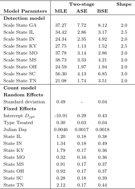
inter-vals. Parameter estimates as well as analytical (ASEs) and bootstrap standard errors

(BSEs) for the best detection and count models are given in Table 2.1. Estimates for

the scale parameter of the hazard-rate detection function stratified by state ranged

between 21.08 (ASE=1.74, BSE=3.51, fixed shape parameter=2.0) for Tennessee and

56.30 (ASE=4.13, BSE=6.85, fixed shape parameter=3.0) for South Carolina.

To calulate a baseline expected number of male indigo buntings within the plot areaa

using the best model, we set the covariates totype = Control,Julian day = 174 (the

mid-point of all days surveyed) andstate = GA. We used the coefficients from Table

2.1 while applying the following transformations (reversing the log-link function of

the Poisson model and convertingbirds/m2 _to_birds/a_{): exp(}₋₁₀_._{91 + 0}_.₀₀₄₆_×_{174 +}

0.5×0.492₎_×_a_{. The last component inside the bracket represents the contribution}

of the random effects term and a = πw2_{. The resulting expected baseline of indigo}

bunting numbers within the plot was 1.43 (BSE=0.59) (or 43.51 (BSE=18.91) birds

perkm2).

The remaining fixed effect coefficients represent proportional changes with respect

to this baseline. The type coefficient for the count model was 0.30 (ASE=0.03,

BSE=0.04) indicating a 35% increase of bird densities on treated fields compared

to control fields. For both models, BSEs were generally larger than ASEs except for

the scale parameters of the detection function for two out of the nine states where

(44)

25

[image:44.612.190.420.247.567.2]

an integrated likelihood approach in chapter 3.

Table 2.1: Maximum likelihood estimates (MLE), analytic (ASE) and bootstrap (BSE) standard errors for model parameters obtained by the two-stage approach for best models. Shape parameters for the one-parameter hazard-rate detection function were fixed.

Two-stage Shape Model Paramters MLE ASE BSE

Detection model

Scale State GA 37.27 7.72 8.12 2.0

Scale State IL 34.42 2.86 3.17 2.5

Scale State IN 24.34 2.35 4.92 2.0

Scale State KY 27.75 1.13 1.52 2.5

Scale State MO 37.78 3.14 2.86 2.0

Scale State MS 38.73 3.33 4.21 2.0

Scale State OH 24.59 1.97 1.94 2.0

Scale State SC 56.30 4.13 6.85 3.0

Scale State TN 21.08 1.74 3.51 2.0

Count model Random Effects

Standard deviation 0.49 - 0.04

Fixed Effects

InterceptDjpr -10.91 0.29 0.43

Type Treated 0.30 0.03 0.04

Julian Day 0.0046 0.0017 0.0018

State IL 1.20 0.18 0.38

State IN 1.34 0.18 0.49

State KY 1.79 0.17 0.36

State MO 0.32 0.16 0.36

State MS 0.91 0.17 0.37

State OH 0.92 0.17 0.37

State SC 0.28 0.18 0.39

(45)

2.4 Case study 2: point transect surveys of

north-ern bobwhite coveys

2.4.1 The data

As part of a study to assess the potential benefits of herbaceous buffers around

agri-cultural fields, Mississippi State University, Department of Wildlife, Fisheries, and

Aquaculture set up a monitoring program using point transects in a number of

Mid-western and Southeastern states in the US (Evans et al., 2013). Similar to case study

1, survey points located at the edge of the field were paired up: one point on a

buffered treatment field and the other on a non-buffered control field of the same

agricultural use and within 1−3km of the treatment point. Each pair of points will

be referred to as a site in the following. Repeat visits were made to each point during

fall of three survey years (2006-2008), and each detected northern bobwhite covey

was recorded along with their estimated radial distance to the point. To facilitate

unbiased distance estimation, observers used satellite images of the point location

and surroundings to mark each detected covey. As this survey did not include

ob-taining estimates of cluster size for each covey, we consider cluster densities (rather

than densities of individuals).

Only those states were included in the analysis that contained more than 50

de-tections of coveys: Georgia, Illinois, Indiana, Iowa, Kentucky, Missouri, Mississippi,

North Carolina, South Carolina, Tennessee and Texas. Within these states, 447 sites

were visited between 1 and 3 times in each survey year. After defining a truncation

distance of 500m following recommendations of Buckland et al. (2001), the analysed

(46)

27

during 2534 counts.

2.4.2 Analysis using the two-stage approach

As distance were measured exactly during the surveys, the first step included fitting

a detection function to observed distances by maximising the likelihood in eqn (2.3).

Preliminary investigation of the distance data indicated that the hazard-rate

detec-tion funcdetec-tion provided a much better fit than the half-normal. In addidetec-tion to the

global model, we included seven different multiple covariate models where the scale

parameter of the hazard-rate detection function was modelled as a function of one,

two or three of the covariates, all possible combinations of including the covariates

state, year and/or type. For these models, the likelihood changed to eqn (2.9) from

page 18.

In a second step, the effective area was incorporated into the density model for λjpr

for which the likelihood is given in eqn (2.7). Parameter estimates were obtained

using the glmer function of the lme4 package (Bates, 2009b) in R. The number of

quadrature points was set to 10 using the argument nAGQ of this function,

follow-ing recommendations of Lesaffre and Spiessens (2001). We explored 16 models that

included a fixed intercept and a random effect for site and combinations of the four

covariates state, type, year and Julian day. Best fitting models for both steps were

found by minimum AIC values.

As the effective area represents an estimate but is included in the model as if it

was a known constant, non-parametric bootstrapping was used to estimate

(47)

estimates. To implement a non-parametric bootstrap routine with 999 repeats, an

automatic model selection was set up in R that included calls to the MCDS engine

from the Distance software (Thomas et al., 2010) for the first step. For each

boot-strap iteration, sites were resampled with replacement until the original number of

sites was obtained (Buckland et al., 2009). To include model uncertainty in inference,

the strategy followed here was to select best fitting models based on minimum AIC

values for each bootstrap iteration (Buckland et al., 1997).

2.4.3 Results

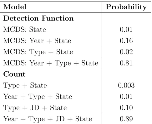
The preferred detection model from the analysis of the original data was the

hazard-rate function that included the covariates year, type and state in the model for the

scale parameter. The preferred count model included all available covariates, i.e.year,

type, Julian day and state. The same models were preferred for the bootstrap

anal-ysis although three other models were selected for both the detection and the count

model with smaller probabilities (Table 2.2). Maximum likelihood estimates as well

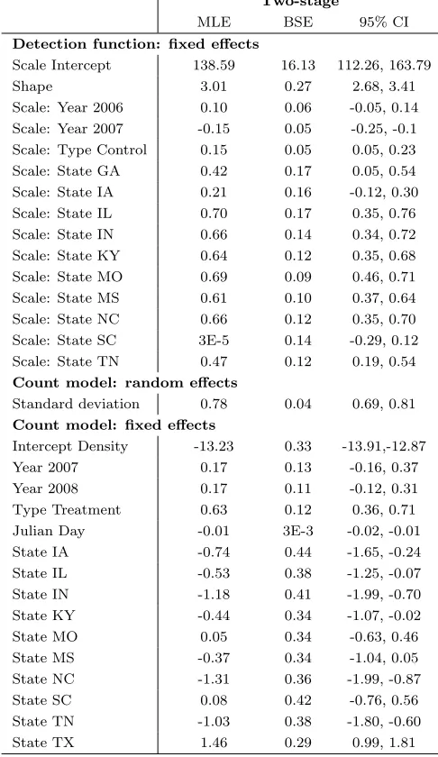
as bootstrap standard errors (BSEs) and 95% confidence intervals are given in Table

2.3. The type coefficient was 0.63 (ASE=0.12) indicating an 88% increase in covey

densities on treated fields compared to control fields. These results will be discussed

(48)

[image:48.612.185.428.344.543.2]

29

Table 2.2: Models and their probabilities resulting from bootstrap analysis. Each count model included a fixed effect intercept and a random effect for site in addition to shown covariates (JD = Julian day). Model probabilities refer to the percentage of times the respective models were chosen during 999 bootstrap iterations.

Model Probability

Detection Function

MCDS: State 0.01

MCDS: Year + State 0.16

MCDS: Type + State 0.02

MCDS: Year + Type + State 0.81

Count

Type + State 0.003

Year + Type + State 0.01

Type + JD + State 0.10

(49)

[image:49.612.182.425.245.665.2]

Table 2.3: Maximum likelihood estimates (MLE), bootstrap standard errors (BSE) and 95% confidence intervals (CI) using the two-stage approach for the models with the highest probabilities (see Table 2.2 for model probabilities). Units of measure-ments were metres for the detection function model and square metres for the count model.

Two-stage

MLE BSE 95% CI

Detection function: fixed effects

Scale Intercept 138.59 16.13 112.26, 163.79

Shape 3.01 0.27 2.68, 3.41

Scale: Year 2006 0.10 0.06 -0.05, 0.14

Scale: Year 2007 -0.15 0.05 -0.25, -0.1

Scale: Type Control 0.15 0.05 0.05, 0.23

Scale: State GA 0.42 0.17 0.05, 0.54

Scale: State IA 0.21 0.16 -0.12, 0.30

Scale: State IL 0.70 0.17 0.35, 0.76

Scale: State IN 0.66 0.14 0.34, 0.72

Scale: State KY 0.64 0.12 0.35, 0.68

Scale: State MO 0.69 0.09 0.46, 0.71

Scale: State MS 0.61 0.10 0.37, 0.64

Scale: State NC 0.66 0.12 0.35, 0.70

Scale: State SC 3E-5 0.14 -0.29, 0.12

Scale: State TN 0.47 0.12 0.19, 0.54

Count model: random effects

Standard deviation 0.78 0.04 0.69, 0.81

Count model: fixed effects

Intercept Density -13.23 0.33 -13.91,-12.87

Year 2007 0.17 0.13 -0.16, 0.37

Year 2008 0.17 0.11 -0.12, 0.31

Type Treatment 0.63 0.12 0.36, 0.71

Julian Day -0.01 3E-3 -0.02, -0.01

State IA -0.74 0.44 -1.65, -0.24

State IL -0.53 0.38 -1.25, -0.07

State IN -1.18 0.41 -1.99, -0.70

State KY -0.44 0.34 -1.07, -0.02

State MO 0.05 0.34 -0.63, 0.46

State MS -0.37 0.34 -1.04, 0.05

State NC -1.31 0.36 -1.99, -0.87

State SC 0.08 0.42 -0.76, 0.56

State TN -1.03 0.38 -1.80, -0.60

(50)

Chapter 3 An integrated likelihood approach

for modelling distance sampling

data with mixed effects

3.1 Introduction

In this chapter, we deal with some of the shortcomings of the two-stage approach

presented in chapter 2 and provide an alternative method, the integrated likelihood

approach. As for the two-stage approach, the motivation for the integrated likelihood

approach also was to replace the design-based component of conventional distance

sampling with a model where animal densities or counts are related to covariates

such as habitat.

However, the shortcoming of the two-stage approach described by Buckland et al.

(2009), and equivalently of the extended version described in chapter 2, is that it

treats the offset, and hence the detection function from the first stage, as known.

(51)

Hence, nonparametric bootstrapping needs to be used to quantify precision of

param-eter estimates, to allow uncertainty from fitting the detection function to propagate

into the second stage.

Royle et al. (2004), on the other hand, developed an integrated likelihood for point

transect data where distances were measured in intervals. These authors combined

a covariate model for the latent variable Np (the true but unknown abundance of

animals at the point) with the cell probabilitiesfi (derived from the detection

func-tion) to model the observed counts npi in the ith distance interval at the pth point.

An advantage of the approach of Royle et al. (2004) is that all model parameters for

both theNp and thefi are estimated in one step. However, Royle et al. (2004) only

assumed a global half-normal detection function where the distance information was

pooled across all points for the respective distance intervals.

Here, we extend the approach of Royle et al. (2004) in the following ways. We model

heterogeneity in detection probabilities and include model selection for thefi model

as well as for the Np. We also extend Royle et al.’s Poisson model by including a

random effect for site in the abundance model to account for correlated counts at the

same sites. This was motivated by our case study 1, the point transects of indigo

buntings, where a large number of sites was included in the analyses and the number

of repeat visits to the same site varied.

In the following we begin by describing our extended version of the integrated

like-lihood of Royle et al. (2004) for both line and point transects (section 3.2), analyse

our case study of indigo buntings using this integrated likelihood and contrast results

with those using the two-stage approach from chapter 2 (section 3.3), and discuss

(52)

33

3.2 Integrated likelihood

As in the previous chapter, we begin by considering a wildlife study that was carried

out at a number of sites, at each of which point or line transects were placed according

to some design and that each site was surveyed at least once following a distance

sampling protocol (see Buckland et al., 2001 or chapter 2 for further details).

If all animals within the search area were detectable with certainty, then observed

counts within the search distance around the line or point would equal the true number

of animals within the search distance around the line (point) and could be modelled

via a log-link using a generalised linear mixed model (GLMM) with a Poisson error

structure (E(Njpr) =λjpr) whereNjpr is the total number of animals present within

the search area ajpr at visitr to line (point) p of site j. The search area ajpr equals

2wljpr for lines (ljpr = length of the respective line) and πw2 for points; in both cases

wrepresents the truncation distance. Combining adjacent lines or points as sites and

including site as a random effect allows (repeat) counts from the same site to covary

without causing bias for the remaining parameters in the model. Theλjpr may then

be modelled by a linear predictor via a log-link function using:

λjpr = exp β0+bj + K

X

k=1

xkjprβk

!

. (3.1)

Here, β0 represents the fixed effect intercept, bj the random effect for site j with

bj ∼ N(0, σb2), xkjpr the observed covariate values for the k = 1,2, ..., K fixed effects

and βk the associated coefficients. In the following β0, ..., βK may be summarised as

Mixed effect models in distance sampling

MIXED EFFECT MODELS IN DISTANCE SAMPLING

Cornelia Sabrina Oedekoven

Abstract

Acknowledgements

Data acknowledgements

Institutional funding acknowledgements

Table of Contents

List of Figures

Chapter 1

Introduction

1.1

Conventional distance sampling

1.2

Recent developments in distance sampling

1.3

Developments of distance sampling methods

proposed in this thesis

Fitting random effects models to

distance sampling data using a

two-stage approach

2.1

Introduction

2.2

The two-stage approach

2.2.1

Heterogeneity in Detection Probabilities

2.2.2

Model Selection

2.2.3

Estimating the Precision

2.3

Case study 1: point transect surveys of indigo

buntings

2.3.1

The data

2.3.2

Analysis using the two-stage approach

2.3.3

Results

2.4

Case study 2: point transect surveys of

north-ern bobwhite coveys

2.4.1

The data

2.4.2

Analysis using the two-stage approach

2.4.3

Results

Chapter 3

An integrated likelihood approach

for modelling distance sampling

data with mixed effects

3.1

Introduction

3.2

Integrated likelihood