Approximate Analysis of Power Offset over Spatially Correlated MIMO Channels

Approximate Analysis of Power Offset over Spatially

Correlated MIMO Channels

Guangwei YU, Xuzhen WANG

School of Information and Communication Engineering, Beijing University of Posts and Telecommunications, Beijing, China

Email:{yuguangwei1982, Gxitao}@gmail.com

Abstract: Power offset is zero-order term in the capacity versus signal-to-noise ratio curve. In this paper, ap-proximate analysis of power offset is presented to describe MIMO system with uniform linear antenna arrays of fixed length. It is assumed that the number of receive antenna is larger than that of transmit antenna. Spa-tially Correlated MIMO Channel is approximated by tri-diagonal toeplitz matrix. The determinant of tri-di-agonal toeplitz matrix, which is fitted by elementary curve, is one of the key factors related to power offset. Based on the curve fitting, the determinant of tri-diagonal toeplitz matrix is mathematically tractable. Conse-quently, the expression of local extreme points can be derived to optimize power offset. The simulation re-sults show that approximation above is accurate in local extreme points of power offset. The proposed ex-pression of local extreme points is helpful to approach optimal power offset.

Keywords: MIMO, multiplexing gain, power offset, high snr region, toeplitz matrix

1. Introduction

Multiple-input multiple-output (MIMO) system is widely used in wireless communication to improve the perform-ance. The spectral efficiency of MIMO channel is much higher than that over the conventional signal antenna channel. The research of MIMO includes two different perspectives: the first one concerns performance analysis in terms of error performance of practical systems, the second one concerns the study of channel capacity.

The design of communication schemes was mainly considered in the former perspectives with the aid of theo-retical analysis and simulation [1][2], and [3]. For the latter, important parameters such as diversity gain [4], multiplexing gain [5][6] (referred to degree of freedom in other literatures), and power offset [7-9], and [10] were emphatically analyzed in the high signal-to-noise ratio (SNR) region. Furthermore, diversity and multiplexing tradeoff has been proposed in [11][12], and [13], that is to say diversity and multiplexing tradeoff can be obtained for a given multiple antenna channel. It is worth pointing out in [11] that the diversity and multiplexing tradeoff is essentially the tradeoff between the error probability and the data rate of a given system.

The multiplexing gain is not sufficient to accurately characterize the property of MIMO capacity. A more ac-curate representation of high SNR behavior in SNR-ca-pacity curve is provided by an affine approximation to capacity, which includes both the multiplexing gain (i.e. slope) and power offset (i.e. zero-order term) [7]. High SNR power offset has been analyzed in [8] over multiple antenna Ricean channels. It was shown in [8] that the

im-pact of the Ricean factor at high SNR region could be conveniently quantified through the corresponding power offset. In [9], high SNR power offset in multiple antenna communication was derived in detail. Achievable through- put was compared between the optimal strategy of dirty paper coding and suboptimal linear precoding techniques (zero-forcing and block diagonalization) in [10] on appli-cation of power offset. Hence, power offset is an impor-tant parameter in multiple antenna communication.

In many practical environments, signal correlation among the antenna array exists due to the scattering. Fad-ing correlation and its effect on the capacity of multiele-ment antenna system has been studied in [14]. Hence, analysis of spatially correlated MIMO channels has been another topic in the past few years, which necessitates the model of correlated channel. A general space-time corre-lation model for MIMO systems in mobile fading channel has been presented in [15]. The model in [15] was flexible and mathematically tractable. In [16], the correlated model of [15] has been used to investigate the capacity of spatially correlated MIMO Rayleigh-fading channels.

Recently, application of different antenna arrays in MIMO system has also been exploited. With the consid-eration of physical constraints imposed by maximum size of the antenna array, uniform linear array of fixed length has been used in [17] to analyze the asymptotic capacity of MIMO systems.

chan-nel, the main result of this paper is the derived expression of local extreme points of power offset, using the uni-form linear array of fixed length. To the best of our knowledge, the main result has not been presented in other literatures.

The rest parts are organized as follows. In Section 2, the basic definitions of multiplexing gain and power offset are presented. System model and correlation model are given in Section 3. Approximate analysis of power offset by fitting determinant curve of tri-diagonal toeplitz matrix is put forward in Section 4. Section 5 shows the simulation results. Finally, a brief conclusion is given in Section 6.

Notation: In the following context, matrices and vectors are denoted by boldface upper case symbols and boldface lower case symbols, respectively. The transpose and Hermitian transpose are denoted by

 

 

 

 is used for the Euclidian norm.

2. Basic Definition

In the high SNR region, the capacity of single-user MIMO system of coherent reception is given by [18][19]

2

( ) min( ,_{T R}) log (1

C SNR  n n SNR o ) (1)

where denote the number of transmit and receive antenna elements , respectively. is the signal to noise ratio. The MIMO capacity in high SNR region is a linear function of , i.e. the stationary slope in SNR-capacity curve. In other words, any increase in

is immaterial, i.e. without any impact to the slope. The slope is the so-called maximum multiplexing gain (degree of freedom).

, T R

n n

, ) T R

n n

SNR

min( ,n n_{T R})

max(

If is fixed to a given value (generally speaking, is less than six, expressed as

T

n

T

n n_T in the following

context), and nRnT, the multiplexing gain equals to a

fixed value without consideration of correlation of chan-nel response and the number of receive antenna elements. So power offset is introduced to compare the impact of channel property with the same value of multiplexing gain, and (1) is replaced by [9]

2

( ) (log ( ) ) (1

(1) 3

dB

C SNR S SNR L o

SNR

S L o

dB

 

 

 

 

 _  _

 

)



(2)

where is multiplexing gain and is power offset in 3-dB units. When ，the multiplexing gain and power offset can be computed by

S_ L_

SNR 

2

( )

lim

log ( ) SNR

C SNR S

SNR

  _ (3)

2

( )

lim log ( ) SNR

C SNR

L SNR

S  _



 

 _  _

  (4)

In the high SNR region, SNR-capacity curve is ap-proximately determined by multiplexing gain and power offset. Most channels, having the same multiplexing gain, may have very different capacities because of various values of the power offset. Hence, power offset is an im-portant parameter to describe the capacity behavior in high SNR region.

3. System Model and Correlation Mode

The system model and channel correlation model are de-fined in this section. For MIMO system, the general baseband model is given by

y Hx n  (5)

where is the channel response matrix, and

is the input complex signal vector whose spatial covariance matrix normalized by the energy per dimension can be expressed as

H

1 2

[  _

T

T n x x x x   ]

 2

( )

1 _{[ ]}

H

T E

E n 

 xx

Φ

x (6)

while and are the

output vector and additive white Gaussian noise vector, respectively. Because of normalization and assumption of isotropic input,

1 2

[ _R]T

n y y y    y

( )

tr

1 2

[ _R T

n n n n   

n ]



T n 

Φ and ΦI_nT , where In is

n n identity matrix.

Kronecker model [16] is used to describe the correla-tion of channel response. On the assumpcorrela-tion of rich scat-tering environments and having no line of sight, the cor-related channel response matrix is denoted by

H  T R

Σ Σ Σ (7) where  is Kronecker product, ΣT and ΣR are

cor-related matrix of transmit and receive antenna, respec-tively. So the channel response matrix H is given by

1 2

R T

 

H Σ HΣ 12 ₍₈₎ where H is channel response matrix whose elements are independent and identical distribution random variables. Without loss of generality, we assume that the distance between transmit antenna elements is large enough to neglect the correlation at the transmit node. Consequently, without considering the antenna correlation at the transmit node, the correlation matrix is identity matrix, and the receive antenna correlation model

T

Σ

R





0

4 4 sin( )

( , )

( )

ij ij

R

I d j d

i j

I

    

 



Σ (9) 0 2 ,

1 R

R R

L J

n

a= æçç_çç p ö÷÷_÷÷ £

-è ø L £10 (12) where L_R is the fixed length of receive antenna array normalized by . In this paper, LR is assumed to be in

the range from 1 to 10. where [0, )

[ , )

is the so-called AOA(angle of arrival),   



  is average value of AOA, d_ij s normalized distance between antenna array elements, that is to say

i

ij ij

d d _ he factual distance between i and j

antenna array element, , d_ij

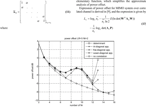
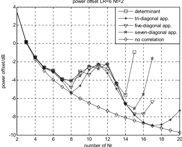
In the Figure 1 and 2, power offset approximation based on tri-diagonal, five-diagonal, and seven-diagonal toeplitz matrix is obtained versus the number of receive antenna with various value of L_R. Furthermore, power offset over independent channel is also provided as lower bound for numerical comparison. It can be seen from Figure 1 and 2 that tri-diagonal toeplitz matrix can be used to approximate the correlation model at the receive node.

is t

 s wave length, i I_n( ) is n-order modified Bessel function. It is obvious that

is real symmetric toeplitz matrix.

( , ) R i j

Σ

On the assumption of isotropic scattering, the correla-tion matrix at the receive node is simplified to

0

( , ) (2 )

R i j J dij

Σ   (10)

4. Approximate Analysis of Power Offset

where is n order Bessel function, and can be simplified to

( )

n

J  Σ_R( , )i j

tri-diagonal toeplitz matrix through the simulation results illustrated by Figure 1 and Figure 2.

Depending on the discussion in Section 3, tri-diagonal toeplitz matrix can be used to approximate the correla-tion model at the receive node. In this seccorrela-tion, the deter-minant curve of tri-diagonal toeplitz matrix is fitted by an elementary function, which simplifies the approximate analysis of power offset.

1

R R

R

n n

Σ

 



 _



 

 _{} 

 



  _{} 

 

_{ }

 

Expression of power offset for MIMO system over corre-lated channel is derived in [9], and the expression is given by

 (11)

 



2

2 1

log (ln det( ))

ln 2 1

log det( )

H

T R

T

T T

L n E

n

n

  



W Λ W

Λ P

(13) where

2 4 6 8 10 12 14 16

-10 -8 -6 -4 -2 0 2 4

number of Nr

po

w

er

of

fs

et

/dB

power offset LR=5 Nt=2

determinant tri-diagonal app. five-diagonal app. seven-diagonal app. no correlation

2 4 6 8 10 12 14 16 18 20 -10

-8 -6 -4 -2 0 2 4

number of Nr

pow

er

of

fs

et

/dB

power offset LR=6 Nt=2

determinant tri-diagonal app. five-diagonal app. seven-diagonal app. no correlation

Figure 2. Approximate analysis of power offset based on 3, 5, and 7 diagonal toeplitz matrix with LR6, nT2 where Λ_T and ΛR are diagonal matrix whose

ele-ments are eigenvalues of Σ_T and Σ_R

Φ

) TP

, respectively. is also diagonal matrix whose elements are eigenvalues of normalized spatial covariance matrix , so is

iden-tity matrix and is constant zero.

P

P



1/nTlog de2 t(Λ

R

Λ can be derived from (11). It is obvious that Λ_R is full rank matrix, and then (13) is simplified to



2

log T ( ( )R ( ))R

L  n  f n g n (14) where f n( )R and g n( )R can be described by



(ln det( )) ( )

ln 2 H R

T

E f n

n

W W

  (15)



ln det( ) ( )

ln 2

R R

T g n

n

  Λ (16)

Because is wishart matrix and nonsingular

with probability 1,

H

W W ( )_R

f n is reduced to [9]





 ₁ 0 1

( ) (log det( ))

ln 2

1 _{( )}

ln 2 T

H

R e

T n

R l T

f n E

n

n l

n 





 

 



W W

(17)

where ( ) is digamma function and the definition of digamma function is

1

1 1

( ) n

l

n

l

   

  



1 1

lim n log_e 0.5772 n

l

n l



 _

 

 _  _





When it comes to function g n( )R , the derivation of ( )_R

g n can be expressed as

 

1 1

( ) ln det( ) ln det( )

ln 2 ln 2

R R R

T T

g n

n n

  Λ   Σ (20)

It can be found from (20) that g n( )_R is only deter-mined by the determinant of ΣR, and the determinant of

R

n order tri-diagonal toeplitz matrix Σ_R can be com-puted by [20].



 











1 1

2 2

1 2

2

2

1 1 4 1 1 4

2 1 4

1 4 0

det

1 2

1 4 0

R R

R

R

n n

n

R R

n n

 

 



 



      



 

    

 _

  

    

Σ (21)

function. When _{1 4 }2_0 in (21), det R

Σ can be ap-proximated by the fitted curve as follow:

2 2

0

( ) 1 5 1 5 (2 )

1 R R

R L

h n J

n

 

   

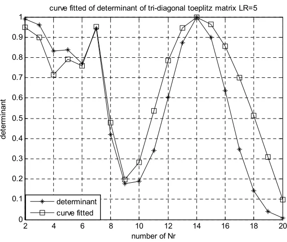
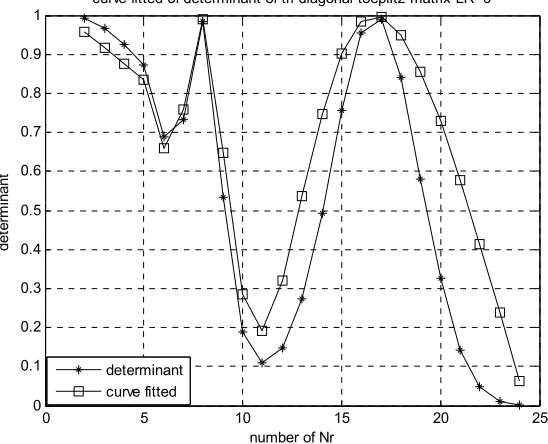
 (22) The approximation between the fitted curves and de-terminant curves of tri-diagonal toeplitz matrix are illus-trated in Figure 3 and Figure 4. From Figure 3 and 4, we can find that the fitting curve can exactly approach the extreme points of the determinant of tri-diagonal toeplitz matrix. However, the expression is much simpler. In other words, the further derivation using the fitted curve is tractable using well-known mathematical software such as WOLFRAM MATHEMATICA.

In the following context, power offset is analyzed in detail. The approximate analysis of power offset is based on the piecewise function of nR . The condition

in (22) is necessary due to , so

the number of receiver antenna 2

1 5  0 detΣ_R 0

R

n can not be large than . Moreover, it shows from the conclusion in [21] that the effect of correlation can be neglected when the normalized length of receive antenna array

4LR1

R L

1 R R n L 

is larger than one wave length, that is to say . Hence, the considered range of the number of receive antenna is

.

1

R R

L  n 4LR1

With the discussion above, when , the

normalized length of receive antenna array

1 R R n L 

R

L is large

than one wave length and the effect of correlation can be neglected, that is to say and the power offset is expressed as

( ) 0R g n 

 

₁ 2

0 1

log ( )

ln 2 T

n T

l T

L n n

n 





 R

l

 



1

(23)

When it comes to the range of , the

normalized length of receive antenna array

1 4

R R R

L  n  L 

R L

( ) 0_R g n 

is smaller than one wave length and the effect of correlation can not be neglected. In other words, . However, for a given value of n_T , the first-order derivative (f n( )_R

( )

is assumed to be continuous) of f nR is obtained by









' 1

0

1

1 0

( ) 1

( )

ln 2

1 _{( )}

ln 2 T

T

n R

R l

R T

n R l T

df n

n l

dn n

n l

n



 







 

 _  _

 

0

   





(24)

where 1( ) is trigamma function. Hence, it shown from (24) that f n( )_R approximately equal to the con-stant (approximation accuracy is related to the value of

C



T

n ). The power offset is expressed as



2

log T ( )R

L  n g n C (25)

2 4 6 8 10 12 14 16 18 20 0

0.1 0.2 0.3 0.4 0.5 0.6 0.7 0.8 0.9 1

number of Nr

de

te

rm

in

an

t

curve fitted of determinant of tri-diagonal toeplitz matrix LR=5

determinant curve fitted

0 5 10 15 20 25 0 0.1 0.2 0.3 0.4 0.5 0.6 0.7 0.8 0.9 1

number of Nr

de te rm in an t

curve fitted of determinant of tri-diagonal toeplitz matrix LR=6

determinant curve fitted

Figure 4. Approximation of determinant of tri-diagonal toeplitz matrix by curve fitting and LR6 Without loss of generality, the constant can be

neglected in the approximate computation. Hence, the power offset in (25) is only determined by

C

( )R

g n

2

. From (22), the curve of the determinant of tri-diagonal toeplitz matrix can be fitted by ( ) 1h nR  5 , where

0 2 ( 1) R R L J n  

 . The first order derivative (h n( )R is

as-sumed to be continuous) of h n( )_R can be computed by

0 1

2

2 2

4 ( ) (

( ) 1 1

( 1) R R R R R R R L L

L J J

dh n n n

dn n    ) R    

 (26)

where LR 1 nR 4LR , that is to say

And then, the second-order derivative of h n( )R can

be computed by

0 1

2

2 3

2 2 2

1

4

2 2

0 0 2

4

2 2

8 ( ) ( )

( ) 1 1

( 1) 2

8 ( )

1 ( 1)

2 2 2

4 ( ) ( ) (

1 1

( 1)

R R

R

R R R

R R R R R R R R R

R R R

R

L L

L J J

d h n n n

dn n

L L J

n n

L L L

L J J J

n n n

n                       _   _   ) 1 R 3 1 2 2 2 1 R L (27) Using (27), the second-order derivative in points

, 1, 2, i

P i  is obtained as follow:

R

n

  _{  }

 . In the range above, function

0 2 ( ) 1 R R J n   L

in (26) has two zero points, i.e.

1 2 2.4048 1 R L    2

1 2 2

2 _2.4048 1

( ) 4.51

: 0 R R L R R n

d h n P

dn  _  L



  ₂  (28)

R

P n



and 2

2 5.5201 1 R R L P n   

 , and

function 1 2 ( ) 1 R R L J n 

 only has one zero point, i.e.

3 2 3.8317 1 R   2

2 2 2

2 5.5201 1

( ) 53.75

: 0 R R L R R n

d h n P

dn  _  L



  ₂  (29)

R

L P

n



 . Consequently, h n( )R has three

extreme points in the range of 2

2 1 R R L n  2

3 2 2

2 _3.8317 1

( ) 17.48

: 0 R R L R R n

d h n P

dn  _  L



 ₂  (30)

2

 _{ }

 

3

,

de-scribed by P i_i, 1, 2, .

With the discussion above, it is obvious that point and are local maximum points of

1

P

2

3

P is local minimum point. Furthermore, it is obvious from (20) that the extreme points of h n( )R is same as

ones of g n( )_R . Consequently, in the range of L_R 1

t

, the extreme points of power offset in (25) can be approximately computed by

4LR1

arg mi

arg ma

R R

n

n





    

P

R

n 



R

n 

 

 

x

, for local mini t

, for local maxi in

L

L 







mal poin

mum po (31)

where is defined as follows:

2 2

1 , 1 , =1, 2,3

R R

i i

L L

i

P P

p p

ìê ú é ùü

ï ï

ï_{ê + ú ê + ú}ï í_{ê ú ê ú}ý

ï ï

ïë û ê úï

î þ

P = (32)

where ê ú_{ë û}x and é ù_{ê ú}x denote the maximum integer smaller than x and minimum integer larger than x,

re-spectively. is the extreme points

com-puted above. (31) can be used to approximately compute the number of receive antenna, in order to achieve the optimal power offset.

, 1, 2,3 i

P i

5. Simulation Results

In the Figure 1 and 2, with the assumption of nT 2,

power offset is approximately analyzed based on tri-di-agonal, five-ditri-di-agonal, and seven-diagonal toeplitz versus the number of receive antenna, with in Figure 1 and in Figure 2. Furthermore, power offset in independent channel is also provided as lower bound for numerical comparison. The approximation trend can be

5 R

L 

6



R

L

found from Figure 1 and 2. The tri-diagonal toeplitz ma-trix can be assumably used to characterize the property of power offset over spatially correlated channel. Hence, tri-diagonal toeplitz matrix can be used to approximate the correlation model at the receive node.

The approximation of fitting the curve of tri-diagonal toeplitz matrix determinant is illustrated in Figure 3 and Figure 4 to compare the difference between fitted curves and determinant curves, with LR 5 in Figure 3 and

6 R

L  in Figure 4. From Figure 3 and 4, we can find that the fitting curve can exactly approach the extreme points of the determinant of tri-diagonal toeplitz matrix. However, the expression is mathematically tractable.

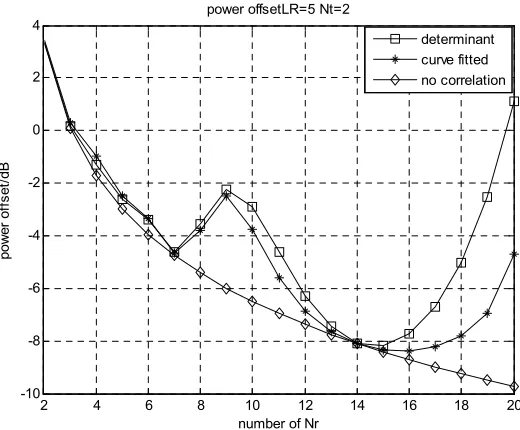
With the same assumption of n_T 2, approximation of power offset is shown in Figure 5 and 6, with LR 5

in Figure 5 and L_R 6 in Figure 6. From Figure 5 and 6, we can find the position of two local minimal points and one local maximum point. With the condition of

5 R

L  and nT 2, the local extreme points computed

by (31) is n_R 9 for local maximum point and

7, R

n  15 6

for local minimal points. With the condition of LR  and nT 2, the local extreme points

com-puted by (31) is n_R 11 for local maximum point and

8, R

n  16 for local minimal points. The computation results based on (31) coincide with the illustration results in Figure 5 and 6. Hence, all the approximation in this paper is reasonable, including approximation of correla-tion model and approximacorrela-tion of determinant of tri-di-agonal toeplitz matrix.

2 4 6 8 10 12 14 16 18 20

-10 -8 -6 -4 -2 0 2 4

number of Nr

pow

er

of

fs

et

/dB

er offsetLR=5 Nt=2 pow

determinant curve fitted no correlation

0 5 10 15 20 25 -12

-10 -8 -6 -4 -2 0 2 4

number of Nr

pow

er

of

fs

et

/dB

power offsetLR=6 Nt=2

determinant curve fitted no correlation

Figure 6. Power offset comparation between accurate and approximate determinant of toeplitz matrix with L_R6, n_T2 Similar results are presented in Figure 7 and 8, with

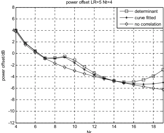
the assumption of and in Figure 7

while in Figure 8. With the condition of

 ₄

T

n  LR 5

8 R

L  L_R 5

and _T 4 9



n

R

, the local extreme points computed by (31)

is for local maximum point and for

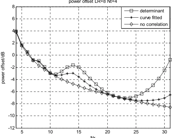
local minimal points. With the condition of

n R  7,

R

L

15



8

n

 and

, the local extreme points computed by (31) is

for local maximum point and for

local minimal points. The computation results based on (31) coincide with the illustration results in Figure 7 and 8.



T

n n

4 14

 

R nR 10,22

Consequently, it is presented in Figure 5 and 7 that the effect caused by the number n_T can be neglected. In other words, for small value of n_T and in the range of

number of receive antenna , the

assumption of

1 4

R R R

L  n  L 1

( )_R

f n C is tenable with neglectable loss of precision. The extreme points of power offset is only determined by g n( )R .

4 6 8 10 12 14 16 18

-12 -10 -8 -6 -4 -2 0 2 4 6 8

Nr

po

w

er

o

ffs

et/d

B

power offset LR=5 Nt=4

determinant curve fitted no correlation

5 10 15 20 25 30 -12

-10 -8 -6 -4 -2 0 2 4 6 8

Nr

po

w

er of

fs

et

/dB

power offset LR=8 Nt=4

determinant curve fitted no correlation

Figure 8. Power offset comparation between accurate and approximate determinant of toeplitz matrix with L_R8, n_T 4

6. Conclusions

Approximate analysis of power offset over spatially cor-related channel is proposed to optimize the number of receive antenna with antenna array of fixed length. An-tenna correlation matrix is approximated by tri-diagonal toeplitz matrix. The determinant of tri-diagonal toeplitz matrix is reduced to simple style by curve fitting with neglectable loss of precision. Based on the approxima-tion above, the expression of local extreme points of power offset is derived. Simulation results shows that the derived expression is accurate in the local extreme points of power offset, that is to say, all the approximation in this paper is reasonable.

REFERENCES

[1] TAROKH V, JAFARKHANI H, CALDERBANK A R. Space-time block code from orthogonal designs. IEEE Transactions on Information Theory, Jul. 1999, 45(5): 1456-1467.

[2] BOUBAKER N, LETAIEF K B, MURCH R D. Performance of BLAST over frequency-selective wireless communication channles. IEEE Transactions on Communication, Feb. 2002, 50(2): 196-199.

[3] LOZANO A, PAPADIAS C. Layered space-time receivers for frequency-selective wireless channels. IEEE Transactions on Communication, Jan. 2002, 50(1): 65-73.

[4] BAKIR L, FROLIK J. Diversity gains in two-ray fading channels. IEEE Transactions on Wireless Communications, Feb. 2009, 8(2): 968-977.

[5] POON A, BRODERSEN R, TSE D. N. C. Degrees of freedom in

multiple-antenna channels: A signal space approach. IEEE Transactions on Information Theory, Feb. 2006, 51(2): 523-536. [6] JAFAR S A, SHAMAI S. Degrees of freedom region of the MIMO X channel. IEEE Transactions on Information Theory, Jan. 2008, 54(1): 151-170.

[7] JINDAL N. High SNR analysis of MIMO broadcast channels. ISIT’05, 2005, 2310-2314.

[8] TULINO A M, LOZANO A, VERDU S. High-SNR power offset in multi-antenna Ricean channels. ICC’05, 2005, 683-687. [9] LOZANO A, TULINO A M, VERDU S. High-SNR power offset

in multi-antenna communication. IEEE Transactions on Information Theory, Dec. 2005, 51(12): 4134-4151.

[10] LEE J, JINDAL N. High SNR analysis for MIMO broadcast channels: Dirty paper coding versus linear precoding. IEEE Transactions on Information Theory, Dec. 2007, 53(12): 4787-4792.

[11] ZHENG L Z, TSE D N C. Diversity and multiplexing: A fundamental tradeoff in multiple-antenna channels. IEEE Transactions on Information Theory, May 2003, 49(5): 1073-1096. [12] TSE D N C, VISWANATH P, ZHENG L Z. Diversity multiplexing tradeoff in multiple-access channels. IEEE Transactions on Information Theory, Sep. 2004, 50(9): 1859-1874.

[13] WAGNER J, LIANG Y C, ZHANG R. On the balance of multiuser diversity and spatial multiplexing gain in random beamforming. IEEE Transactions on Wireless Communication, Jul. 2008, 7(7): 2512-2525.

[15] ABDI A, KAVEH M. A space-time correlation model for multielement antenna systems in mobile fading channels. IEEE J. Select. Areas Communication, Apr. 2002, 20: 550-560. [16] CHIANI M, WIN M Z, ZANELLA A. On the capacity of

spatially correlated MIMO Rayleigh Fading channels. IEEE Transactions on Information Theory, Oct. 2003, 49(10): 2363-2371.

[17] WEI S, GOECKEL D, JANASWAMY R. On the asymptotic capacity of MIMO systems with antenna arrays of fixed length. IEEE Transactions on Wireless Communications, Jul. 2005, 4(4): 1608-1621.

[18] TELATAR I E. Capacity of multi-antenna Gaussian channel. Europe Transactions on Telecommunication, Nov./Dec. 1999, 10: 585-595.

[19] FOSCHINI G J, GANS M J. On the limits of wireless communications in a fading environment when using multiple antenna. Wireless Personal Communication, 1998, 6(3): 315-335. [20] XU Z, ZHANG K Y, LU Q. Fast algorithm based on toeplitz

matrix. Xi’an: Northwest Industrial University, 1999.