C
2014. The American Astronomical Society. All rights reserved. Printed in the U.S.A.
SUBARCSECOND IMAGING OF THE NGC 6334 I(N) PROTOCLUSTER: TWO DOZEN
COMPACT SOURCES AND A MASSIVE DISK CANDIDATE
T. R. Hunter1, C. L. Brogan1, C. J. Cyganowski2,3, and K. H. Young2 1NRAO, 520 Edgemont Road, Charlottesville, VA 22903, USA;[email protected]
2Harvard-Smithsonian Center for Astrophysics, Cambridge, MA 02138, USA
3SUPA, School of Physics and Astronomy, University of St. Andrews, North Haugh, St. Andrews KY16 9SS, UK
Received 2014 March 3; accepted 2014 May 1; published 2014 June 6
ABSTRACT
Using the Submillimeter Array (SMA) and Karl G. Jansky Very Large Array, we have imaged the massive protocluster NGC 6334 I(N) at high angular resolution (0.5 ∼ 650 AU) from 6 cm to 0.87 mm, detecting 18 new compact continuum sources. Three of the new sources are coincident with previously identified H2O masers. Together with the previously known sources, these data bring the number of likely protocluster members to 25 for a protostellar density of∼700 pc−3. Our preliminary measurement of theQ-parameter of the minimum spanning tree is 0.82—close to the value for a uniform volume distribution. All of the (nine) sources with detections at multiple frequencies have spectral energy distributions consistent with dust emission, and two (SMA 1b and SMA 4) also have long wavelength emission consistent with a central hypercompact Hiiregion. Thermal spectral line emission, including CH3CN, is detected in six sources: LTE model fitting of CH3CN (J=12–11) yields temperatures of 72–373 K, confirming the presence of multiple hot cores. The fitted LSR velocities range from−3.3 to−7.0 km s−1, with an unbiased mean square deviation of 2.05 km s−1, implying a protocluster dynamical mass of 410±260M. From analysis of a wide range of hot core molecules, the kinematics of SMA 1b are consistent with a rotating, infalling Keplerian disk of diameter 800 AU and enclosed mass of 10–30M that is perpendicular (within 1◦) to the large-scale bipolar outflow axis. A companion to SMA 1b at a projected separation of 0.45 (590 AU; SMA 1d), which shows no evidence of spectral line emission, is also confirmed. Finally, we detect one 218.4400 GHz and several 229.7588 GHz Class-I CH3OH masers.
Key words: accretion, accretion disks – Hii regions – ISM: individual objects (NGC 6334 I(N)) – ISM: kinematics and dynamics – stars: formation – stars: protostars
Online-only material:color figures
1. INTRODUCTION
Massive star formation is a phenomenon of fundamental importance in astrophysics yet a detailed understanding of it has been elusive (Zinnecker & Yorke2007). The present state of theory and numerical simulation research fall into two major categories of processes: “core accretion” and “competitive accretion,” as recently reviewed by Tan et al. (2014). In the core accretion scenario, massive stars (like low-mass stars) are formed via the collapse of self-gravitating, centrally condensed cores. These cores are discrete structures within the larger-scale molecular cloud, and each core constitutes the mass reservoir for a single star or small multiple system. As a result, core mass maps directly to stellar mass, and the core mass function maps to the stellar initial mass function (e.g., Myers et al. 2013; Krumholz et al.2009; McKee & Tan 2003, and references therein). In contrast, competitive accretion models are intrinsically models of star cluster formation. Fragmentation in a cluster-scale gas clump produces many low-mass protostars, which then accrete (competitively) from the large-scale gas reservoir. In this picture, massive starsmust form in a cluster environment, and massive stars and their surrounding clusters must form simultaneously (e.g., Bonnell & Smith2011; Smith et al.2009, and references therein).
There are several significant observational constraints that these theories must face. First, there is mass segregation—the fact that the most massive members of young clusters are concentrated in the center (e.g., Kirk & Myers 2011). It remains unclear whether this property is primordial or a result
the possibility of interaction between massive protostars, as well as their probable impact on low-mass protostars forming in their midst. Furthermore, given the deeply embedded nature of protoclusters, sensitive high dynamic range millimeter and centimeter imaging will be needed to obtain an accurate census of their low-mass membership.
A third observational constraint on theory is the tentative yet growing evidence for massive Keplerian accretion disks around massive protostars. Discovered through subarcsecond angular resolution imaging, there is a steadily increasing number of massive disk candidates around central stars of varying mass
M∗. Examples of disk candidates with an enclosed mass ofM∗ ≈
7–10Minclude IRAS 20126+4104, IRAS 18360−0537, and
Orion KL Source I (Cesaroni et al. 2005; Xu et al. 2012; Qiu et al. 2012; Hirota et al. 2014). Larger-scale structures (toroids) with diameters of several thousand AU have also been reported, which may encompass either an O-type protostar or a cluster of massive protostars (e.g., Beltr´an et al.2011; Zapata et al.2010). There are also cases of apparent sub-Keplerian rotation (AFGL2591-VLA3: Wang et al. 2012) as well as of a lack of Keplerian rotation signatures on 500 AU scales (NGC 7538 IRS1: Beuther et al.2013). Most of the candidate disks show a strong bipolar molecular outflow perpendicular to the disk plane, analogous to low-mass protostellar disk/
outflow systems. It is important to note that the presence of such disks does not immediately favor either the core accretion or competitive accretion model, as they are expected to exist under both scenarios. However, as our knowledge of the massive disk population grows, both theories are certain to face new challenges.
To further explore the protostellar population of massive protoclusters, we have been pursuing detailed observations of the nearby examples in NGC 6334, a region containing multiple sites of high mass star formation (Straw and Hyland1989; Persi & Tapia2008; Russeil et al.2010). A recent deep near- and mid-infrared survey revealed over 2200 young stellar object (YSO) candidates, and subsequent estimates of the star formation rate suggest that it may be undergoing a “mini-starburst” event (Willis et al.2013). At the northeastern end of the region, the deeply embedded source “I(N)” was first identified at 1 mm by Cheung et al. (1978) and later detected at 400μm by Gezari (1982), who estimated a size of 50. Single-dish observations of high velocity SiO emission indicated significant outflow activity at this location (Megeath & Tieftrunk1999). Our initial Submillimeter Array (SMA) observations of NGC 6334 I(N) at ∼2 resolution resolved a Trapezium-like protocluster of seven compact millimeter continuum sources within a projected diameter of 0.1 pc (Hunter et al. 2006; Brogan et al. 2009). As revealed by the millimeter spectral line data (Brogan et al. 2009), the brightest three continuum sources (SMA 1, SMA 2, and SMA 4) are the origin of the hot core line emission seen in the many single-dish molecular line observations of this source (Kuiper et al.1995; Thorwirth et al.2003,2007; Walsh et al. 2010; Kalinina et al. 2010). Hot NH3 was resolved by 1.5 resolution Australia Telescope Compact Array observations of the (5, 5) and (6, 6) lines, which peak toward SMA 1 (Beuther et al. 2007a). The profile of the (6, 6) line showed a double peak separated by∼4 km s−1, which was interpreted as possibly tracing a rotating circum-protostellar disk (Beuther et al.2007a). With similar angular resolution, Brogan et al. (2009) detected a comparable velocity gradient toward SMA 1 in a few other hot core molecules. However, Karl G, Jansky Very Large Array (VLA) 7 mm continuum observations with a 0.5 beam resolved
SMA 1 into multiple components (Brogan et al.2009; Rodr´ıguez et al.2007), making the larger-scale velocity gradient difficult to interpret.
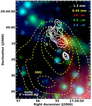
The NGC 6334 I(N) millimeter protocluster is embedded in a region that is remarkably dim in the mid-infraredSpitzerimages, and has the characteristics of an Infrared Dark Cloud. To provide an overview, Figure 1 reprises the millimeter and infrared continuum imaging results from Brogan et al. (2009). Despite the millimeter multiplicity, we identified only some extended 4.5μm emission associated with the bipolar outflows from SMA 1, 4 and 6, and a single 24μm point source near SMA 4 (Brogan et al.2009; Hunter et al.2006). In contrast, our VLA detection of copious amounts of 44 GHz Class I CH3OH maser emission to the southeast of the compact millimeter continuum sources is indicative of outflow activity (Cyganowski et al. 2009; Kurtz et al.2004; Voronkov et al.2014), specifically in the area surrounding the single-dish (sub)millimeter continuum source SM2 (Sandell 2000). Similarly, our VLA H2O maser observations revealed 11 locations of emission, only 8 of which were associated with the known compact millimeter continuum sources, suggesting the presence of additional YSOs (Brogan et al.2009).
In this paper, we present new subarcsecond SMA 1.3 mm, 0.87 mm and VLA 6 cm imaging that indeed reveals significant further multiplicity in this protocluster, as well as the detailed kinematics of the hot cores and complex spectral energy distri-butions (SEDs). The details of the observations are summarized in Section2, while Sections3and4present our key results and discussion, respectively. For the distance to NGC 6334 I(N), we adopt 1.3 kpc based on recent H2O maser parallax studies: 1.34+0.15
−0.12 kpc (Reid et al.2014) and 1.26+0−0..3321 kpc (Chibueze et al.2014). In the past, the most commonly used value was 1.7 kpc from photometric estimates for the NGC 6334 region (Neckel1978; Pinheiro et al.2010), implying a reduction by a factor of 1.7 for derived quantities based on the distance squared, such as mass and luminosity. For example, the total luminos-ity of NGC 6334 I(N) as measured by Sandell (2000) is now 1.0×10³L
with this revised distance.
2. OBSERVATIONS
The details of the SMA4 1.3 mm and 0.87 mm observations and the NRAO5 VLA 6 cm observations are summarized in Table 1. The very extended (henceforth, VEX) 1.3 mm SMA data were calibrated in MIRIAD (Sault et al. 1995), then exported to CASA (McMullin et al. 2007) where the continuum was subtracted to create a line-only VEX data set. The continuum is then composed of the line-free portions of the data set. Self-calibration was performed on the continuum data, and solutions were transferred to the line data. Line cubes were generated with a channel spacing of 1.1 km s−1 and robust weighting of 1.0, with the exception of the 218.44 and 229.76 GHz Class I methanol maser transitions, which were imaged with robust weighting of 0.0. The flux calibration is based on Titan, Ceres, and SMA flux monitoring of the observed quasars and is estimated to be accurate to within 20%. The same procedure was also followed for the VEX 0.87 mm data. Unfortunately, the observing conditions for the 0.87 mm data
4 The Submillimeter Array (SMA) is a collaborative project between the Smithsonian Astrophysical Observatory and the Academia Sinica Institute of Astronomy and Astrophysics of Taiwan.
Figure 1.Overview of the NGC 6334 I(N) region in the mid-infrared. The three-color image was generated from theSpitzerMIPSGAL and GLIMPSE survey images at 24, 4.5, and 3.6μm (Benjamin et al.2003; Churchwell et al.2009; Carey et al.2009). For reference the SMA compact + extended (COMP+EXT) configuration 1.3 mm continuum with 2.2×1.3 resolution from Brogan et al. (2009) is shown in white contours (levels=40, 80, 160, 320, 640 mJy beam−1). The dashed yellow contours show the JCMT 0.45 mm emission (14resolution) from Sandell (2000) (levels: 60, 80, 100, 120, 160 Jy beam−1). The labeled 0.45 mm contour indicates the position of the single-dish source SM2 reported by Sandell (2000).
(A color version of this figure is available in the online journal.)
were significantly worse than for the 1.3 mm data in terms of higher winds and more variable opacity, leading to greater phase instability. As a result, the 0.87 mm spectral line cubes are too noisy to be useful.
Two 1.3 mm continuum images were constructed: (1) to maximize the continuum sensitivity and minimize artifacts from resolved out structure, the VEX 1.3 mm continuum data were combined with the extended configuration (henceforth, EXT) continuum data presented in Hunter et al. (2006) and Brogan et al. (2009) and imaged with robust weighting of 0.5. Note that the EXT 1.3 mm data only cover a portion of the spectral coverage of the VEX data so no such combination was possible for the line data. The relative weight of the individual visibilities between the two configurations is such that the angular resolution of the combination is similar to that of the VEX data alone. This “EXT+VEX” continuum image was used to identify and characterize the 1.3 mm dust continuum sources; it is not sensitive to smooth structures larger than about 9. (2) In an effort to better match theuv-coverage of the VEX 0.87 mm data, the line-free portions of the VEX 1.3 mm data were imaged withuv-spacings>90kλand robust=0 weighting. This image is henceforth termed the “VEX-UV” 1.3 mm continuum image. The 0.87 mm continuum image was also created two ways,
both using a robust weighting of 1.0: (1) a version using all of the data to obtain good angular resolution and sensitivity; and (2) a version with a 300 kλ uv-taper to better match the VEX 1.3 mm data, which was then subsequently convolved to the same resolution as the VEX-UV 1.3 mm continuum image. Thisuv-tapered and convolved image was used to determine the 0.87 mm dust continuum properties. The 0.87 mm images are not sensitive to smooth structures larger than about 3. All measurements from all images were obtained from versions that had been corrected for the primary beam response.
The VLA data were calibrated in CASA with scripts based on the VLA pipeline.6Imaging and self-calibration were performed manually in CASA. The flux calibration accuracy is estimated to be 10%. Due to the large primary beam (nearly 10), the VLA 6 cm data include the bright ultracompact Hii region NGC 6334 F as well as the 45diameter Hiiregion NGC 6334 E (Rodr´ıguez et al. 2003), which are both located south of the field of interest. We thus imaged a large field (107 pixels) containing these objects in order to minimize the confusion toward NGC 6334 I(N). Comparing the new 6 cm JVLA data to the 1.3 cm and 7 mm VLA data presented in Brogan et al. (2009;
Table 1
Parameters of the New Observations
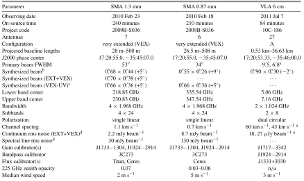
Parameter SMA 1.3 mm SMA 0.87 mm VLA 6 cm
Observing date 2010 Feb 23 2010 Feb 18 2011 Jul 7
On-source time 240 minutes 210 minutes 84 minutes
Project code 2009B-S036 2009B-S036 10C-186
Antennas 7 6 27
Configuration very extended (VEX) very extended (VEX) A
Projected baseline lengths 28 m–508 m 26.5 m–508 m 0.53 km–36.63 km
J2000 phase center 17:20:55.0,−35:45:07.0 17:20:55.0,−35:45:07.0 17:20:53.33,−35:46:00.0
Primary beam FWHM 53 34 9.5, 6.8a
Synthesized beamb 0.68×0.44 (+5◦) 0.55×0.26 (+9◦) 0.90×0.30 (−2◦)
Synthesized beam (EXT+VEX) 0.70×0.39 (+5◦) · · · ·
Synthesized beam (VEX-UV)c 0.66×0.36 (+5◦) 0.66×0.36 (+5◦) · · ·
Lower band center 218.85 GHz 335.54 GHz 5.06 GHz
Upper band center 230.83 GHz 347.54 GHz 7.16 GHz
Bandwidth 4×1.968 GHz 4×1.968 GHz 2×1.024 GHz
Subbands 4×24 4×24 2×8
Polarization single linear single linear dual circular
Channel spacing 1.1 km s−1 0.7 km s−1 60 km s−1, 43 km s−1 a
Continuum rms noise (EXT+VEX)d 2.2 mJy beam−1 8.7 mJy beam−1 18, 27μJy beam−1 a
Spectral line rms noised 30 mJy beam−1 130 mJy beam−1 · · ·
Gain calibrator(s) J1733−1304, J1924−2914 J1733−1304, J1924−2914 J1717−3342
Bandpass calibrator 3C273 3C273 J1924−2914
Flux calibrator(s) Titan, Ceres Ceres J1331+3030
225 GHz zenith opacity 0.07 0.03–0.06 n/a
Median wind speed 2 m s−1 5 m s−1 3 m s−1
Notes.
aThe first number is for the 5 GHz data; the second number is for the 7 GHz data.
b This is the angular resolution of the 1.3 mm spectral line cubes, 0.87 mm continuum image, and 5 and 7 GHz continuum images (convolved to the same resolution), respectively. The position angle in degrees east of north is given in parentheses.
cThe 1.3 mm image was generated from theuvspacings>90kλ, and the 0.87 mm image was generated with auv-taper of 300 kλand then convolved to the same resolution as the 1.3 mm VEX-UV image.
dMeasured at the center of the primary beam.
see also Rodr´ıguez et al.2007), we found a∼0.4 disagreement in the astrometry between the old and new data. The most likely culprit was the phase calibrator used in the older VLA observations of J1720−358 (B1717−358). We alerted both VLA and ALMA to our suspicion, which led to an ALMA calibration observation of J1720−358 using the nearby VLBA calibrator J1717−3342 (Petrov et al.2006) at Band 3 (92 GHz) as the reference source with 24 antennas (2013 October 29, execution blocks: uid://A002/X70c186/X12, X25, and X4a). As a result of these observations, the ALMA calibrator database has been updated with a revised position of 17:20:21.798±0.030, −35:52:48.128±0.010 (a correction of 0.43; as of this writing the VLA calibrator database has not yet been updated). We have used this new information to correct the astrometry of the 1.3 cm and 7 mm images used in this paper. We note that our H2O maser observations used J1717−3342 as the phase calibrator (Brogan et al.2009) and thus do not require correction.
3. RESULTS
3.1. Continuum Emission
3.1.1. 1.3 mm Continuum
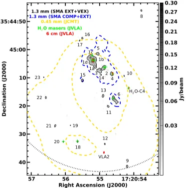
The 1.3 mm EXT+VEX image of the continuum emission is shown in Figure 2. All of the seven previously identified millimeter sources (Brogan et al. 2009) are detected, with the exception of one of the fainter, more extended sources (SMA 7), whose emission is apparently resolved out by the longer baselines employed in these observations. We detect
Figure 2.SMA 1.3 mm EXT+VEX continuum with 0.7×0.39 resolution in grayscale and a single black solid contour at 4.5σ=10 mJy beam−1. The dotted circle marks the 25% level of the southern edge of the primary beam—although we searched for sources out to 20% level, none were found beyond this radius. The labels correspond to the source names in Tables2and3. The image used in this figure was not corrected for the primary beam response, but all measurements, including Table2, were taken from the corrected image. The JVLA 6 cm continuum data is shown as a single red contour at 80μJy beam−1(4.5σ). For ease of comparison with previous work and Figure1, the single dashed blue contour shows the 40 mJy beam−1level of the COMP+EXT SMA 1.3 mm continuum and the dashed yellow contour shows the 60 and 100 Jy beam−1levels of the JCMT 0.45 mm continuum. The green crosses mark the H2O masers from Brogan et al. (2009).
each source with a two-dimensional (2D) Gaussian to find the peak position and integrated flux density and attempt to find the deconvolved size. For 9 of the 24 sources, the fitted size was well constrained in both the major and minor axes, and we can compute the brightness temperature (a lower limit to the physical temperature). For 11 sources, the minor axis was not well constrained, and the geometric mean of the major and minor axes of the fitted Gaussian was less than that of the synthesized beam (0.5). Four sources were consistent with a point source in both axes. For the latter two cases, we assign 0.5 as an upper limit to the size and use this to compute a lower limit to the brightness temperature. With the exception of the 24μm source near SMA 4, which likely traces hot dust in the walls of the cavity formed by the outflow from that source (e.g., De Buizer & Minier2005), none of the millimeter continuum sources have counterparts in the mid-infraredSpitzerimages (Brogan et al. 2009).
3.1.2. 6 cm to 7 mm Continuum and Revised Astrometry
The VLA 6 cm image (Figure2) shows two previously known 6 cm point sources, associated with SMA 1 and SMA 4 (Carral
et al. 2002), plus two new sources that are not associated with 1.3 mm emission. All four sources are consistent with unresolved compact sources with sizes <0.3. Their positions and flux densities are listed in Table3. One of the new sources coincides within 0.054 (70 AU) with the centroid of H2O maser component C4 (Brogan et al.2009), hence we call it H2O-C4. The other new source is located≈30(0.2 pc) south of SMA 1. Because it is not coincident with any maser or 1.3 mm source, we call this source VLA 2 in order to distinguish it from both the 1.3 cm source VLA-K1 reported by Rodr´ıguez et al. (2007; outside the SMA field of view) and the 7 mm source VLA 3 reported by Brogan et al. (2009; which was named for its proximity to SMA 3 and yet of independent nature).
Table 2
Observed Properties of the 1.3 mm Continuum Sources
Sourcea,e Fitted Position (J2000) Peak Intensityb Peak Fitted Flux Fitted Size (Pos. Angle E of N)c Fitted Size T brightness
α(h m s) δ(◦ ) (Jy beam−1) S/N Density (Jy) ×(◦) (AU) (K)
SMA 1a 17:20:55.137 −35:45:05.76 0.0866±0.0022 39 0.225±0.020 0.99±0.05×0.52±0.10 (+35±5) 1300×680 10±2 SMA 1b+d 17:20:55.192 −35:45:03.93 0.3257±0.0022 148 1.059±0.076 1.02±0.05×0.74±0.06 (+128±9) 1300×960 32±4 SMA 1c 17:20:55.267 −35:45:02.89 0.1384±0.0022 63 0.335±0.024 0.74±0.05×0.61±0.07 (+141±25) 960×790 17±3 SMA 2 17:20:54.870 −35:45:06.40 0.1039±0.0022 47 0.169±0.007 0.58±0.03×0.27±0.07 (+138±6) 750×350 24±6 SMA 3 17:20:55.003 −35:45:07.40 0.0331±0.0022 15 0.138±0.016 1.06±0.06×0.93±0.09 (+10±25) 1400×1200 3.2±0.5
SMA 4 17:20:54.627 −35:45:08.73 0.0425±0.0022 19 0.059±0.004 <0.5 <650 >5.4
SMA 5 17:20:55.043 −35:45:01.53 0.0433±0.0022 20 0.053±0.002 0.68±0.01×0.51±0.03 (+6±1) 890×660 4.9±0.3
SMA 6 17:20:54.590 −35:45:17.40 0.1812±0.0022 82 0.285±0.016 <0.5 <650 >26
SMA 7 undetected · · · ·
SMA 8 17:20:53.782 −35:44:46.16 0.0297±0.0034 8.7 0.046±0.003 <0.5 <650 >4.4
SMA 9 17:20:54.196 −35:45:41.45 0.1070±0.0054 20 0.139±0.006 <0.5 <650 >13
SMA 10 17:20:54.283 −35:45:09.38 0.0115±0.0022 5.2 0.025±0.003 <0.5 <650 >2.2
SMA 11 17:20:54.751 −35:45:20.18 0.0197±0.0022 9.0 0.043±0.004 0.72±0.07×0.27±0.15 (+76±25) 940×350 5.0±2.5
SMA 12 17:20:54.849 −35:45:33.51 0.0312±0.0034 9.2 0.039±0.004 <0.5 <650 >3.5
SMA 13 17:20:54.900 −35:45:16.41 0.0425±0.0022 19 0.049±0.004 <0.5 <650 >4.4
SMA 14 17:20:54.962 −35:45:08.92 0.0130±0.0022 5.9 0.022±0.002 0.49±0.09×0.39±0.11 (+104±25) 640×510 2.7±0.9
SMA 15 17:20:55.504 −35:45:10.96 0.0469±0.0022 21 0.063±0.003 <0.5 <650 >5.8
SMA 16 17:20:55.503 −35:44:55.90 0.0179±0.0022 8.1 0.031±0.004 <0.5 <650 >2.8
SMA 17 17:20:55.590 −35:44:56.89 0.0145±0.0022 6.6 0.021±0.003 <0.5 <650 >1.9
SMA 18d 17:20:55.645 −35:45:32.61 0.0433±0.0034 13 0.043±0.003 <0.5 <650 >3.9
SMA 19 17:20:55.854 −35:45:26.98 0.0179±0.0025 7.2 0.024±0.004 <0.5 <650 >2.1
SMA 20 17:20:56.061 −35:45:32.66 0.0320±0.0034 9.4 0.032±0.003 <0.5 <650 >2.4
SMA 21 17:20:56.298 −35:45:27.04 0.0362±0.0034 11 0.052±0.004 <0.5 <650 >4.7
SMA 22 17:20:56.571 −35:45:17.01 0.0263±0.0025 11 0.042±0.003 0.58±0.05×0.31±0.10 (+2±4) 750×400 5.5±1.9
SMA 23 17:20:56.629 −35:45:09.84 0.0167±0.0025 6.7 0.017±0.002 <0.5 <650 >1.5
Notes.
aSMA 1–7 were previously detected in Brogan et al. (2009).
bThe intensity of the peak pixel; uncertainties correspond to the image rms in the annular region in which the source is located (see Section3.1.1). cDeconvolved from the beam.
dPosition consistent with SM2 from Sandell (2000).
[image:6.612.335.551.464.643.2]eQuantities in columns labeled “Fitted” were obtained from the CASA imfit task.
Table 3
Observed Properties of the 6 cm Continuum Sources
Source Fitted Position (J2000)a Peak Intensity (mJy beam−1)b
α(h m s) δ(◦ ) 5.06 GHz 7.16 GHz
SMA 1b 17 20 55.192 −35 45 03.83 0.327±0.014 0.373±0.019 SMA 4 17 20 54.619 −35 45 08.57 0.157±0.014 0.235±0.026 H2O-C4c 17 20 54.149 −35 45 13.70 0.110±0.011 0.091±0.019 VLA 2c 17 20 54.871 −35 45 36.49 0.102±0.014 0.133±0.041
Notes.
aObtained from a 2D Gaussian fit to the image.
bThe intensity of the peak pixel; measured from the image corrected for primary beam response and convolved to 0.9×0.3 beam.
cNewly detected cm sources.
astrometry of those images are given in Table 4. With the new astrometry, there is now very good agreement between the VLA and SMA continuum contours for the primary millimeter sources (SMA 1b+d, 4, and 6). The angular separation between SMA 1b and 1d in the 7 mm image is 0.45 (590 AU) at a position angle of−67◦(east of north). The area surrounding SMA 6 is shown in Figure4. The peaks of the 7 mm, 1.3 mm and 0.87 mm emission are in good agreement. There is an extended ridge of 1.3 mm emission to the southwest, part of which may arise from a distinct source. However, because it is not clearly separated from SMA 6 and there is no compact counterpart at any other wavelength, we have not identified this ridge as a separate object.
Table 4
Revised Positions of the 1.3 and 0.7 cm Continuum Sources
Source Fitted Position (J2000)a
α(h m s) δ(◦ )
1.3 cm
SMA 1b 17 20 55.185 −35 45 03.98
SMA 1c 17 20 55.259 −35 45 02.88
SMA 1d 17 20 55.222 −35 45 04.08
SMA 4 17 20 54.616 −35 45 08.66
0.7 cm
SMA 1a 17 20 55.150 −35 45 05.71
SMA 1b 17 20 55.190 −35 45 03.95
SMA 1c 17 20 55.255 −35 45 02.91
SMA 1d 17 20 55.223 −35 45 04.12
VLA 3 17 20 54.992 −35 45 06.92
SMA 4 17 20 54.618 −35 45 08.71
SMA 6 17 20 54.591 −35 45 17.39
Note.aThese positions were extracted from Gaussian fits to images corrected for the position error of the phase calibrator J1720−358 in the VLA catalog, as described in Section2. The uncertainties on the absolute fitted positions are0.03.
3.1.3. 0.87 mm Continuum
[image:6.612.43.296.467.541.2]Figure 3.Zoom on the central portion of the NGC 6334 I(N) protocluster including SMA1, SMA2, SMA3, and SMA4. The SMA 1.3 mm EXT+VEX continuum image is in grayscale and black contours (levels: 10, 24, and 66 mJy beam−1). The red contours are the 6 cm VLA image (levels: 80, 144, and 200μJy beam−1). The blue contours show the 7 mm VLA continuum (levels: 0.63, and 0.84 mJy beam−1). The yellow contours show the 1.3 cm VLA continuum (levels: 0.23 and 0.35 mJy beam−1). The green crosses mark the centroid positions of H2O masers from Brogan et al. (2009). The synthesized beams are shown in the lower left corner coded by contour color; the 7 mm beam is not shown as it is very similar to the SMA 1.3 mm beam (black; see Table1).
along with the H2O maser positions observed with a beam of 0.79×0.25 at P.A. =+7◦ (Brogan et al.2009) and the first moment of the CH3CN J = 12–11, K = 7 transition. With higher resolution than the 1.3 mm VEX image, the 0.87 mm image clearly indicates that SMA 1d is a source of submillimeter emission separate from SMA 1b. Further evidence that these are distinct sources comes from the H2O maser positions: the vast majority are coincident with SMA 1b while none are seen toward SMA 1d (see also Chibueze et al.2014). The position angle of the spatial extent of the H2O masers is somewhat inclined to that of the large-scale bipolar outflow axis measured in SiO 5–4 (Brogan et al.2009). Also, the kinematics are complicated, and reminiscent of the H2O maser system of radio source I in Orion BN/KL (see, e.g., Greenhill et al. 2013) in terms of spatial extent (∼500 AU) and the apparent overlap of widely disparate velocities. Similar to the H2O emission, the CH3CN emission is centered on SMA 1b (see Section3.2), with no measurable emission coming from SMA 1d.
In an attempt to apportion the 1.3 mm continuum flux density between SMA 1b and 1d, we fit a single 2D Gaussian to SMA 1b in the 1.3 mm VEX-UV continuum image. The residual image showed a weak source of unresolved emission coincident with the 7 mm and 1.3 cm source SMA 1d. To estimate the flux density of this source, we fit the residual image with a single Gaussian, which yielded a point source of 44±8 mJy at the J2000 position: 17:20:55.23 ± 0.07, −35:45:04.14 ± 0.07. The angular separation of this position from SMA 1b is
0.56±0.04 at position angle−69◦ ±10◦, in good agreement with the 7 mm separation between SMA 1b and 1d. Finally, we estimate the flux density of SMA 1b alone to be the joint flux density of SMA 1b+d from Table2minus the value for SMA 1d, or 1.02±0.08 Jy. A similar procedure was then performed on the 0.87 mm image, yielding a flux density of 100±25 mJy for SMA 1d.
Eight of the 1.3 mm sources are detected in the uv-tapered 0.87 mm image. Note that 10 of the 16 non-detected sources (including VLA 2) lie beyond the one-third sensitivity radius of the primary beam, where the 4.5σ limit is >0.12 Jy beam−1. Using this image, the fitted positions, flux densities, and sizes are listed in Table5. We caution that theuv-tapered 0.87 mm image is still not sensitive to the largest angular scales that the 1.3 mm EXT+VEX image contains. Therefore, the 0.87 mm flux densities should be taken as lower limits for those sources having 1.3 mm fitted sizes significantly larger than 0.5, partic-ularly those located in the complicated central cluster. For the 1.3 mm sources smaller than 0.5 and located away from the central cluster (including SMA 13 and SMA 15), the 0.87 mm measurements are unlikely to suffer from missing flux and may be considered to be accurate.
3.2. Hot Core Line Emission
Figure 4.Zoom on the SMA 6 region. The SMA 1.3 mm EXT+VEX continuum image is shown in grayscale and black contours (levels: 10 (4.5σ), 24, 66 mJy beam−1). The magenta contours show the tapered and convolved (to match 1.3 mm) SMA VEX 0.87 mm continuum (levels: 75 (3σ at this point in the primary beam), 150, and 300 mJy beam−1). The blue contours show the 7 mm VLA continuum (levels: 0.63 (3σ) and 95 mJy beam−1). The green crosses mark the centroid positions of the three groups of H2O masers from Brogan et al. (2009). The synthesized beams are shown in the lower left coded by contour color; the 1.3 mm and 0.87 mm resolutions are the same (black).
[image:8.612.92.522.495.691.2]Table 5
Observed Properties of the 0.87 mm Continuum Sources
Sourced Fitted Position (J2000) Peak Intensitya Fitted Fluxb Fitted Size (Pos. Angle E of N)c Fitted Size T brightness
α(h m s) δ(◦ ) (Jy beam−1) Density (Jy) ×(◦) (AU) (K)
SMA 1c 17:20:55.269 −35:45:02.88 0.296±0.014 0.63±0.03 0.63±0.03×0.42±0.05 (+113±10) 820×550 24±3 SMA 1b+d 17:20:55.194 −35:45:03.98 0.801±0.014 1.67±0.08 0.62±0.03×0.36±0.06 (+129±8) 810×470 76±14 SMA 2 17:20:54.871 −35:45:06.43 0.230±0.014 0.27±0.02 0.64±0.03×0.43±0.04 (+164±2) 830×560 9.9±1.2 SMA 4 17:20:54.626 −35:45:08.73 0.125±0.015 0.13±0.02 0.65±0.02×0.38±0.04 (+178±2) 850×490 5.4±0.7
SMA 5 17:20:55.048 −35:45:01.42 0.061±0.016 0.06±0.02 <0.5 <650 >3.5
SMA 6 17:20:54.595 −35:45:17.40 0.461±0.020 0.66±0.04 <0.5 <650 >41
SMA 13 17:20:54.883 −35:45:16.32 0.107±0.018 0.28±0.03 <0.5 <650 >17
SMA 15 17:20:55.511 −35:45:11.07 0.107±0.016 0.19±0.04 <0.5 <650 >12
Notes.
aThe intensity of the peak pixel.
bDue to the difference inuvcoverage, these values should be considered lower limits when compared to the 1.3 mm flux densities in Table2, except for SMA 13 and 15. The uncertainties do not include the overall calibration uncertainty of 20%.
cDeconvolved from the beam.
[image:9.612.47.571.290.445.2]dQuantities in columns labeled “Fitted” were obtained from the CASA imfit task.
Table 6
Properties of Spectral Lines Shown in Figure6
Species Transition Frequency Elower Integrated Intensity (Jy beam−1*km s−1)c
(GHz) (K) Cataloga,b SMA1b SMA2 SMA4 SMA6 SMA15 SMA18
HC3N J=24–23 218.32479 120.5 JPL 7.49±0.22 <0.65 2.48±0.22 1.52±0.38 <0.74 2.90±0.41
OCS J=18–17 218.90336 89.3 CDMS 4.71±0.21 1.38±0.21 2.64±0.21 2.03±0.28 0.6±0.2 2.36±0.36 13CS J=5–4 231.22069 22.2 CDMS 2.06±0.30 1.22±0.30 2.06±0.30 1.02±0.29 <0.70 <1.54 CH3OH (E) 80,8–71,6 220.07849 86.1 CDMS 5.45±0.33 3.16±0.33 4.48±0.33 2.04±0.32 <0.79 <1.27 CH3OH (E) 201,19–200,20 217.88639 497.9 CDMS 3.68±0.22 1.07±0.22 2.63±0.22 <0.86 <0.84 <1.31 CH3OH vt=1 (A) 61,5–72,6 217.29920 363.5 CDMS 4.40±0.28 1.61±0.28 3.47±0.28 <0.87 <0.86 <1.72 CH3CN J=12–11,K=3 220.70902 122.6 JPL 6.08±0.27 2.56±0.27 3.29±0.27 1.87±0.35 <0.80 2.63±0.39 CH3CN J=12–11,K=7 220.53932 408.0 JPL 2.63±0.22 <0.65 <0.65 <0.74 <0.49 <1.08 CH3CH2CN 252,24–242,23 220.66092 132.4 CDMS 4.34±0.29 <0.88 <0.88 <0.71 <0.66 <1.18 CH3OCHO (A)d 201
,20–191,19 216.96590 101.1 JPL 5.75±0.28 4.34±0.28 2.53±0.28 2.03±0.35 <0.99 <1.52
CH3OCH3 172,15–163,14 230.23376 136.6 JPL 3.19±0.23 1.23±0.23 1.06±0.23 <0.72 <0.63 <1.25
HNCO 101,10–91,9 218.98101 90.6 CDMS 5.28±0.23 2.13±0.23 2.07±0.23 0.85±0.27 <0.89 <1.44
Notes.
aCDMS=http://www.astro.uni-koeln.de/cgi-bin/cdmssearch bJPL=http://spec.jpl.nasa.gov/ftp/pub/catalog/catform.html
cThe integrated intensity was measured from moment zero images; upper limits are 3σ.
dThis transition is blended with three other CH3OCHO transitions with the same line intensity andElower. The velocity separations from this reference transition are +1.57,−0.48, and−2.10 km s−1, which is less than half of the total velocity gradient in SMA 1b.
and SMA 18 to a lesser extent. At the current sensitivity, 1.3 mm spectral line emission is not detected toward any of the other cores. The spectral line emission is dominated by spatially com-pact emission from complex molecules. Indeed, most of the more abundant species that exhibited outflow emission (e.g., CO,13CO, SiO, DCN, etc.) in the lower resolution SMA data presented in Brogan et al. (2009) are mostly resolved out in the very extended configuration data. As a result, the channels with these molecules have significantly higher noise (by factors of 3–10) due to imaging artifacts caused by the lack of short spacing information. From the 8 GHz of available 1.3 mm spec-tral bandwidth we identified for detailed analysis 12 transitions from 9 different chemical species that are representative of the range of line emission morphologies, kinematics, and line excitation temperatures detected in these data, and further-more do not suffer significant line blending (see Table6 for more details). First moment images of these transitions toward the central region of the cluster are shown in Figure6, where the field of view is the same as Figure3. The parent cube was made with Briggs weighting and a robust parameter of 1.0. Details of
the transitions shown are provided in Table6, including their rest frequencies, excitation energies, and integrated intensities. The first striking feature in the images is the velocity gradient across the central 0.8 (1000 AU) of SMA 1b, which is seen consistently in all transitions. The orientation and magnitude of the velocity gradient is comparable to that seen at∼2 angu-lar resolution (Brogan et al.2009). In the lower energy lines such as HC3N and OCS, the emission and its accompanying gradient also extend somewhat to the northeast toward SMA 1c. A zoomed view of the CH3CNK= 7 transition is shown in Figure 5(b). The magnitude of the gradient ranges from 3 to 5 km s−1 arcsec−1, with the largest values seen in the lines of CH3OH and CH3OCHO. The position angle of the gradient was measured in each transition by viewing the data cube in CASA, marking the RA/Dec centroid of the emission in the outer ve-locity channels, and computing the corresponding slope. The median and standard deviation of the position angle taken over all the transitions is−52◦±5◦.
Figure 6.Images of the first moment of the 12 spectral lines listed in Table6from the SMA VEX 1.3 mm data. The field of view is the same as Figure3. The excitation energy (in Kelvin) of the lower level of each transition is indicated. The black contours show the 1.3 mm EXT+VEX continuum emission (contour levels: 10, 24, and 66 mJy beam−1). The arrow in the lower left panel indicates the cut used to generate the pv diagrams in Figure11. The resolution of the EXT+VEX continuum and VEX line data is similar (see Table1); the beamsize is shown in the lower left corner of the lower left panel.
(A color version of this figure is available in the online journal.)
detections indicate differences in both chemistry (HC3N being detected in SMA 4 but not SMA 2) and excitation conditions (SMA 2 being more extended in the lower energy transitions). Also, the central velocity of the emission in SMA 1b differs by several km s−1 from the emission seen toward SMA 2 and SMA 4, indicating a significant velocity dispersion in this protocluster. To better quantify the characteristics of the line emission and estimate the gas physical conditions, we extracted theJ=12–11 CH3CN spectra at the peak positions of all the continuum sources in Table2. Only six sources show detectable emission; in particular, there is no sign of emission
from SMA 1c or 1d. We used the CASSIS7package to perform a local thermodynamic equilibrium (LTE) model fit to the CH3CN and CH133 CN ladders, which provide a good measurement of gas temperature in hot cores (e.g., Pankonin et al.2001; Araya et al. 2005). There were five free parameters in the model: temperature, velocity, line width, column density, and diameter. Based on the galactocentric distance of NGC 6334, we assume a12C:13C ratio of 58 (Milam et al.2005). We used the Markov Chain Monte Carlo (MCMC)χ2 minimization option, which
Table 7
Best Fit CASSIS LTE Models to the CH3CN Spectra
Source Temperature Diameter Column Density Linewidth LSR Velocity H2Densitya
(K) () (AU) (cm−2) (km s−1) (km s−1) (cm−3)
One-component models
SMA 1b 143±7 0.38±0.01 490 (3.94±0.34)E17 4.72±0.01 −3.29±0.01 8E9
SMA 2 140±6 0.30±0.01 390 (4.26±0.72)E16 4.40±0.07 −7.01±0.02 1E9
SMA 4 208±2 0.26±0.01 340 (6.26±0.20)E16 8.79±0.04 −6.80±0.02 2E9
SMA 6 95±3 0.25±0.01 330 (9.39±0.32)E16 4.26±0.15 −4.91±0.10 3E9
SMA 15 72±15 0.22±0.03 290 (3.76±0.46)E16 3.76±0.46 −6.36±0.37 1E9
SMA 18 139±10 0.25±0.02 330 (4.77±0.51)E16 5.71±0.36 −4.94±0.16 1E9
Two-component models
SMA 1b comp. 1 80±5 0.40±0.02 520 (4.51±0.31)E17 3.21±0.15 −3.24±0.17 9E9
SMA 1b comp. 2 307±40 0.24±0.02 310 (2.89±0.27)E17 6.63±0.52 −3.35±0.17 9E9
SMA 4 comp. 1 135±5 0.30±0.01 390 (3.06±0.25)E16 4.78±0.66 −8.25±0.07 8E8
SMA 4 comp. 2 280±35 0.22±0.02 290 (3.31±0.51)E16 6.85±0.38 −2.67±0.19 1E9
Note.aDerived from the CH3CN column density assuming spherical geometry and a CH3CN:H2abundance of∼1×10⁻⁸.
is far more CPU time-efficient and tractable than a uniform grid search. Unlike a grid search, the MCMC search begins with an initial guess and a range for each parameter, and makes random steps in each parameter in order to explore the range. The amplitude of the random step size is initially large but decreases during the first stage of the computation as the space is explored. In the latter stage, smaller steps are used to refine the best chi-squared potential. In order to establish the parameter space for each source and the initial guess, we ran initial executions with very broad ranges in order to encompass plausible values. Based on these results, we narrowed the ranges somewhat. The typical search parameters were ranges of±60 K for cool sources and ±100 K for warm sources in temperature,±2 km s−1 in linewidth,±3 km s−1 in velocity, and a factor of 10–50 in column density (all centered on the initial guess), and a range of 0.1–0.5 for angular diameter. With these ranges, we ran several executions of MCMC each with a different value of the automatic step size reduction factor (called reducePhysicalParam), thereby achieving a variety of acceptance rates in the range of 0.2–0.4 after 2000 iterations. The cutoff parameter, which determines when the step size reduction factor becomes fixed, was set to half the number of iterations.
The best fit values reported in Table 7 are taken from the execution that achieved an optimal acceptance rate of≈0.25. To obtain realistic uncertainties for the parameters, we take the standard deviation from this single execution and add (in quadrature) half the total spread in the individual best fit model values. The best-fit model spectra are overlaid on the observed spectra in Figure7. In the case of SMA 4, the line shapes are clearly non-Gaussian and a single component fit yields an abnormally high line width of>8 km s−1. For this source, we also performed a two-component fit, which resulted in smaller, more reasonable line widths from two spatially unresolved components that have rather different temperatures and velocities (by 6 km s−1). This result may indicate the presence of an unresolved binary hot core system. For SMA 1b, we also found that two temperature components produced a better fit to the low and high-K lines of the spectrum, as is typical of many hot cores (e.g., Hern´andez-Hern´andez et al. 2014; Cyganowski et al.2011). In this case, the search range for the cooler component was 60–150 K, and for the hot component
was 150–600 K. The best-fit temperature of the hot component of SMA 1b being in excess of 300 K is consistent with the detection of theK=10 component withElower =771 K. The final column in Table7provides an order-of-magnitude estimate of the volume density of H2that was calculated from the fitted column density assuming spherical geometry and an assumed CH3CN abundance of 1×10⁻⁸. This value is intermediate between the extrema of recent measurements of the CH3CN abundance in hot cores, which range from 1×10⁻⁷to 1×10⁻⁹ (see, e.g., Remijan et al. 2004; Hern´andez-Hern´andez et al. 2014). A comparison of the CH3CN column density to the dust column density is discussed further in Section4.4.
3.3. Maser Action in Two 1.3 mm CH3OH Lines
Probable maser emission in the Class I 229.75881 GHz CH3OH (8−1,8–70,7) E transition is a conspicuous feature of recent SMA observations of massive protostellar outflows (e.g., Cyganowski et al. 2012, 2011, and references therein). In these outflows, the 229 GHz emission is generally co-located (spatially and spectrally) with lower frequency Class I masers. In NGC 6334 I(N), we observe strong features in both the 229 GHz transition and the Class I 218.44005 GHz (10−5,5–11−4,8) E transition at the position of the brightest 44 GHz maser (spot 55 of Brogan et al.2009), which also coincides in velocity and position with the−3 km s−124.9 GHz CH
Figure 7.In each panel, the black spectrum is the observed spectrum toward the indicated source in units of brightness temperature (corrected for primary beam response), and the red spectrum is the best fit single-component CASSIS LTE model of CH3CN and CH13
3CNJ=12–11. The blue spectrum shown for SMA 1b and SMA 4 is a two-component model. The corresponding model parameters are given in Table7. In the SMA 1b panel, the vertical lines below the spectrum mark the frequencies of theKcomponents of CH3CN (solid lines) and CH13
3CN (dotted lines). The rest frequency of13CO is also marked by the vertical dashed line. The flat tops on many of the lowKlines are indicative of high optical depths.
Table 8
Observed and Derived Parameters of the 218 and 229 GHz CH3OH Maser Emission Componentb Fitted Position (J2000)a Peak Intensity Flux Density Deconvolved T
B vLSR
α(h m s) δ(◦ ) (Jy beam−1) (Jy) Size (×) (K)c (km s−1)
229.75881 GHz (8−1,8–70,7) E transition
1 (8) 17 20 54.327 −35 45 22.31 0.76 1.51±0.12 <0.5 145 −7.56±0.06 2 (9) 17 20 54.392 −35 45 22.68 0.57 1.91±0.13 <0.5 180 −8.66±0.13 3 (11) 17 20 54.447 −35 45 22.76 1.46 3.19±0.15 0.67×0.23 480 −7.65±0.07 4 17 20 54.589 −35 45 10.33 0.79 2.18±0.22 0.80×0.42 150 −2.66±0.06 5 (22) 17 20 54.925 −35 45 13.70 1.25 1.45±0.18 <0.5 >140 −5.56±0.06 6 (25) 17 20 54.952 −35 45 13.99 0.84 1.98±0.11 0.82×0.15 380 −5.15±0.07 7d 17 20 55.048 −35 45 14.89 0.76 0.84±0.06 0.39×0.12 420 −5.73±0.08 8d 17 20 55.024 −35 45 15.32 0.60 1.60±0.07 0.82×0.42 110 −5.15±0.06 9d(55) 17 20 55.670 −35 45 00.38 6.40 8.80±0.16 0.44×0.15 3100 −3.03±0.01
218.44005 GHz (10−5,5–11−4,8) E transition
9 (55) 17 20 55.671 −35 45 00.34 2.28 3.09±0.12 <0.5 270 −3.07±0.03
Notes.
aThe fitted position of the component in the channel of peak emission.
bA number in parentheses indicates that the corresponding 44 GHz CH3OH maser component from Table 4 of Brogan et al. (2009) is within 0.2 of this position.
cThe brightness temperature (TB) is computed from the integrated flux density and the deconvolved size. When the deconvolved size is an upper limit, the beam size is used (0.71×0.37 for the 218.4400 GHz line, and 0.67×0.36 for the 229.7588 GHz line).
dThis component is within 0.3 of a 24.9 GHz CH3OH maser (Beuther et al.2005).
seen toward the hot cores. Seven of the nine components are within 0.2 of a 44 GHz maser (Brogan et al.2009) and/or within 0.33 of a 24.9 GHz CH3OH maser (Beuther et al.2005). All nine have brightness temperatures greater than the energy level of the transition. In both transitions, fainter emission appears toward the continuum sources SMA 1, SMA 2, and SMA 4.
[image:12.612.93.523.428.598.2]Figure 8.Image of the EXT+VEX 1.3 mm continuum in grayscale and black contours, (same three contours as in Figure3). The field of view is identical to Figure2. The integrated intensity of the SiOJ=5–4 emission from the COMP+EXT SMA data presented in Brogan et al. (2009) is shown in gray contours, indicating strong outflow emission. The positions of the various CH3OH masers are marked as follows:×: 229.76 GHz; square: 218.44 GHz; + : 44 GHz; diamond: 24.9 GHz (Beuther et al.2005); five-pointed star: the intensity-weighted centroid of the six 6.7 GHz masers (17:20:54.619,−35:45:08.66) computed from the table in Walsh et al. (1998). The positions and velocities of the newly discovered Class I 218.44 and 229.76 GHz CH3OH masers are tabulated in Table8.
(A color version of this figure is available in the online journal.)
229 GHz line, and the other lies at 17:20:53.781,−35:45:13.58 (J2000) with an LSR velocity of−1.3 km s−1.
4. DISCUSSION
4.1. Nature of the Continuum Sources
Nine of the continuum sources are detected at more than one wavelength. To explore the nature of these objects, we have constructed the SEDs in Figure 9. Two of the objects, SMA 1b and SMA 4, are detected longward of 1.3 cm, and their SEDs are well-described by a combination of free–free emission plus dust emission. The other seven sources all show a steeply rising spectral index in the submillimeter. Note, because the existing 3 mm observations (Beuther et al.2008) have more than four times poorer angular resolution than the other wavelengths presented here, it is not possible to separate the contributions to the 3 mm flux density for the individual components of SMA 1. Additionally, the 3 mm flux densities for SMA 4 and SMA 6 are regarded as upper limits for the size scales considered here. Further details on individual sources are described below along with descriptions of the modeling procedure.
4.1.1. SMA 1b and SMA 4
Figure 9.Spectral energy distributions of the nine continuum sources detected at more than one wavelength. The 6 cm, 1.3 mm, and 0.87 mm measurements are from this paper, while the rest can be found in Brogan et al. (2009). The flux density error bars represent the formal error of the two-dimensional Gaussian model fit plus a fraction of the total flux density (to account for the typical calibration uncertainty, see Section2). Non-detections are shown as 3σupper limits. The 3 mm flux density measurements for SMA 4 and SMA 6 (Brogan et al.2009) are regarded as upper limits for the size scales considered here. The lower limits drawn for the detections at 0.87 mm are due to the relative lack of short spacings compared to the 1.3 mm measurements. In SMA 1b and SMA 4, the dotted curve is a free–free emission model (ne∝r−2: Olnon1975) whose parameters are listed in the lower right, the dashed curve is the dust model, and the solid curve is the sum. The parameters of the dust
emission model are listed in the upper left of each panel. For SMA 1c, 1d, 5, and 13, the dashed and dotted curves areT=50 K andT=20 K dust, respectively.
alone. Nevertheless, the prior evidence that these are high-mass protostars (Brogan et al.2009) leads us to favor the HCHii
interpretation.
To model HCHii region emission, we have used the bremsstrahlung emission model V of Olnon (1975) in which the electron density profile follows a power-law distribution (ne(r)∝r−2) transitioning to a sphere of constant density
em-bedded in the center, which avoids a non-physical singularity. This formulation yields a spectral index of +0.6 at frequencies below the turnover point, which provides a good match to the SEDs of known hypercompact Hiiregions (Franco et al.2000). To determine the optimal model, we used the “lmfit” Python package,8which performs nonlinear least square minimization
8 http://lmfit.github.io/lmfit-py
using the Levenberg–Marquardt algorithm. Because the free–free emission and dust emission are comparable at fre-quencies just above the free–free turnover point, it is best to model both emission mechanisms simultaneously. To model the dust emission, we use a single-temperature modified gray-body function (Rathborne et al.2010; Gordon1995). With six flux density measurements, we attempted to model five free pa-rameters, including three for the central sphere of the HCHii
Unfortunately, simultaneous fits to all five parameters are not very constraining due to degeneracies between the parameters. Instead, we defined a 16 by 16 point grid of electron density (105–108 cm−3) and temperature (4000–14,000 K), and fit the remaining three parameters at each grid point. The grid points were uniformly distributed—logarithmically for density and linearly for temperature. For SMA 1b, 15% of the results reproduced all the flux density measurements well and had rather similarχ2 values. For SMA 4, 23% of the results were in this category. The rest of the combinations of parameters were notably deviant at one or more data points. In Figure9, we plot the curve corresponding to the median parameter values and report the standard deviation of the five parameters across the good fits. For SMA 1b, the dotted curve corresponds to
ne0=6×105cm−3and a diameter ofd=44 AU. The expected FWHM of the total HCHiiemission (i.e., including the portion outside the central sphere) is then 54 AU. The corresponding values for SMA 4 are 1.6×107cm−3andd =7 AU, yielding a FWHM of 9 AU. Both of these sizes are consistent with being unresolved by our beam. Therefore, one explanation for these objects is that they are currently in the gravitationally trapped phase of HCHii evolution (Keto 2007, 2003). If so, then in the spherical accretion flow model, the measured radius of an HCHii must be less than the Bondi–Parker transonic radius, which in turn places a lower limit to the central stellar mass (see Equation (3) of Keto 2007). Using a sound speed of 11 km s−1 for 10,000 K gas, the corresponding lower limits for the central stars in SMA 1b and SMA 4 are 4.4 and 1.4M, respectively. Of course, the presence of ionizing radiation required to form the HCHii implies a central stellar mass of∼8M or more. Evidently, the accretion flow is still sufficiently strong to maintain the ionization radius significantly inward of the point where pressure-driven expansion can begin, and these stars can potentially continue to gain mass.
4.1.2. SMA 1c
In addition to a dust component, this source shows excess emission at 1.3 cm, the nature of which remains unclear. There is no significant compact spectral line emission coincident with this source; the moment images of HC3N, OCS and13CS give the impression that emission avoids it and wraps around it (Figure6). More sensitive observations at wavelengths longward of 2 cm are needed to understand the nature of the centimeter continuum emission. To model the dust emission, we use the 7 mm and 1.3 mm flux densities and the assumed temperature range for the gas (20–50 K, Section 3.2). Because only two flux densities are available (as is the case for SMA13 and 15), we cannot fit forβ andτ1.3 mmsimultaneously. Instead, we first established a±1σ range forβ by a Monte Carlo treatment of the flux densities and their uncertainties. We then derive the corresponding range ofτ1.3 mmby solving the graybody model at each combination of theTandβextrema to find the value of
τ1.3 mmthat matches the 1.3 mm flux density measurement. We report the minimum and maximum of the resulting values as the
τ1.3 mmrange in the text labels of Figure9.
4.1.3. SMA 1d
SMA 1d is perhaps the most intriguing source as it shows a consistent spectral index from 1.3 cm to 0.87 mm. With measurements at four wavelengths available, we used “lmfit” to fit the spectral index of +2.25± 0.07. This slope is only marginally steeper than an optically thick blackbody, and is similar to the values recently reported in the low-mass class
0 protostar L1527 (Tobin et al.2013) and in source VLA2 in the high mass star-forming core AFGL2591 (van der Tak et al. 2006). If this emission arises from dust, then, as summarized by Tobin et al. (2013), it could be explained by large dust grains (compared to the wavelength), non-isothermal conditions, or optically thick structure, in which case it must be very compact. A similar spectral index is seen in the source NGC 6334 I-SMA4 (Hunter et al. 2013), suggesting that it arises from a not uncommon phase of evolution of massive star formation. An alternative to dust is the core of an optically thick jet (Reynolds 1986), in which the outer parts of the jet are too faint to detect at the current sensitivity level. Again, more sensitive and higher resolution observations are needed to explore these possibilities.
4.1.4. SMA 2, SMA 6, SMA 5, SMA 13, and SMA 15
The rest of the continuum sources that are detected at 1.3 mm and 0.87 mm but not at longer wavelengths almost certainly arise from dust emission. If they were free–free emission, the allowed range of spectral index (−0.1 for optically thin emission to +2 for optically thick emission) would make them easily detectable in the VLA images. As described in Section3.1.3, our 0.87 mm measurements of SMA 13 and SMA 15 do not suffer from missing flux, and their steep spectral indices from 1.3 mm to 0.87 mm are consistent with thermal dust. However, we must consider the chances of these sources being extragalactic background objects dominated by dust emission. The South Pole Telescope (SPT-SZ) survey of 771 deg2in three frequency bands provides a good reference point for comparison (Mocanu et al.2013). From their cumulative distribution plot, the number of SPT detections with dust-like SEDs that are brighter than 25 mJy at 220 GHz is only 0.25–0.40 deg−2. The probability of encountering such a source in the field of view of Figure2 is only 5×10⁻⁶. Thus, it is safe to conclude that these are not background objects, but are members of the protocluster. In the case of SMA 2 and SMA 5, although the spectral indices are consistent with dust emission, we can only place lower limits on
β: 1.0 and 0.5, respectively (based on the upper limits at 1.3 cm and the lower limits at 0.87 mm).
4.1.5. VLA 2 and H2O-C4
Regarding the two new 6 cm point sources (VLA 2 and H2O-C4) that are not detected in millimeter continuum, the fact that one of them (H2O-C4) coincides with a H2O maser is compelling evidence that it is tracing a protostellar object, due to the strong association of molecular outflows with H2O masers (Szymczak et al.2005; Codella et al.2004; Tofani et al.1995). In fact, it is the fourth brightest of the 11 H2O masers in the region, with an isotropic luminosity of 1.6×10⁻⁶L
, which is characteristic of massive young stellar objects (MYSOs) (e.g., Cyganowski et al.2013) and the high end of intermediate-mass YSOs (e.g., Bae et al. 2011). In the Urquhart et al. (2011) Red MSX Source survey, which includes over 300 H2O maser measurements, the bolometric luminosities of MYSOs with this maser luminosity range from 102–105 L, suggesting that H2O-C4 is amassiveprotostellar object.
spectral index of−0.7 (Condon et al.2012), we find an expected source density of 4.5×10⁵sr−1. Multiplying by the solid angle of Figure2, we calculate a 6.3% chance of finding a source in the range of 0.05–0.15 mJy. Thus, the most likely scenario is that VLA2 resides in the protocluster and may trace some form of YSO. Given the lack of millimeter continuum and maser emission, the centimeter emission could also arise from a low-mass, pre-main sequence (PMS) star in which any associated circumstellar dust emission is too faint to be detected. Such objects have been seen, for example, in the Cepheus A East star-forming region (Hughes1988; Garay et al.1996) at a distance of 700 pc (Dzib et al.2011). The variable sources (HW 3a, 8, 9) emit 0.15–3.0 mJy at 6 cm and show no point source counterparts in SMA 0.87 mm images (Brogan et al.2007). At the distance of NGC 6334 I(N), the 6 cm flux densities of these objects would be 0.04–0.9 mJy, a range that includes both VLA2 and H2O-C4. It is interesting to note that HW 8 and HW 9 are both X-ray sources with HW 8 postulated to be a pre-main sequence star (due to its high median photon energy), while the softer, brighter, and more variable HW 9 is consistent with activity on a B-type star (Schneider et al.2009). In NGC 6334 I(N), a recentChandraX-ray survey finds seven sources in the field of Figure2, but none of the detections correspond in position to within 1.5 of any of the millimeter or centimeter sources, and their 1σ X-ray position uncertainties are0.3 (Feigelson et al. 2009).
4.2. Protocluster Structure and Statistics
The unprecedented multiplicity of sources in this field allows us to quantitatively analyze the structure of a young massive protocluster for the first time. First, we define the membership of the protocluster by requiring either the detection of compact millimeter continuum emission or the positional coincidence of at least two star formation indicators. Starting with the source list of Table 2, we exclude SMA 7 as there is no compact component detected. Of the two new 6 cm sources, we can include only the H2O maser source H2O-C4. VLA 2 could be protostellar, but lacking a second positive indicator we exclude it. Finally, although we have presented strong evidence that SMA 1b and 1d are independent sources, they may form a binary system. Our sensitivity to binaries is clearly limited by our angular resolution, so we choose to count these two objects as a single source in order to avoid biasing the following statistics by double counting some binaries but not others. The final tally of sources is thenNtotal=25. The area of the protocluster on the sky is limited by the 1.3 mm primary beam. The largest angular radius from the phase center of a detected source at 1.3 mm is 33, whereσ(r) ≈5.4 mJy beam−1. This implies that our sample of 1.3 mm compact sources in this region is complete down to 25 mJy across a physical radius of 0.21 pc corresponding to a projected area of 0.14 pc2 and a spherical volume of 0.038 pc3. The presence of 25 sources within this volume yields an average number density of 660 pc−3. We note that only 20 of the sources are above the 25 mJy completeness threshold; therefore, this computed density is strictly a lower limit even if the underlying population does not extend beyond the faintest detection. In other words, due to the radial decrease in sensitivity, the faintest sources detected in the central portion of the field would have been missed in the outer portions of the field.
Following the techniques applied to infrared and optical observations of clusters of stars and Hiiregions (e.g., Pleuss et al.2000; Schmeja & Klessen2006), we have constructed the
Figure 10.Minimum spanning tree of the protocluster as defined by the 24 detected sources in Table2plus the water maser/6 cm source H2O-C4 from Table3. The origin is the mean position of all sources. The filled points are the six sources for which we were able to measure the LSR velocity (Table7). The horizontal dashed lines demarcate the seven 10wide strips in which the protostars were counted (from north to south: 1, 2, 6, 9, 3, 3, 1) in order to compute the effective distance to be used in the calculation of the dynamical mass in Section4.3by the method of Schwarzschild & Bernstein (1955).
minimal spanning tree (MST) formed from these 25 sources, as shown in Figure 10. The minimum spanning tree for a set of points is defined as the set of edges connecting them that possesses the smallest sum of edge lengths. To compute it, we used a python function based on the algorithm of Prim (1957). From this result, we compute theQ-parameter, which is defined as the ratio ofm¯, the normalized mean edge length of the MST, to ¯
s, the correlation length, which is defined as the mean projected separation between sources normalized by the cluster radius,
Rcluster (Cartwright & Whitworth 2004). Rcluster is defined as the distance from the mean position of all the stars to the furthest star from that point. For this cluster, we obtainRcluster= 31.95 and:
Q=m¯
¯
s =
6.024/
√
Ntotalπ R2cluster
(Ntotal−1)
19.93/Rcluster =
0.510
0.623 =0.82. (1)
Interestingly, this value (0.82) is close to the critical value that separates clusters between the regime of multiscale (fractal) substructure (Q <0.8) typified by the Taurus and Chamaeleon clusters, and a centrally concentrated configuration typified byρ
Oph and IC348 (Cartwright & Whitworth2004). It is also close to the value of 0.84 obtained for stars in the Orion Trapezium Cluster (Kumar & Schmeja 2007). In the smoothed particle hydrodynamics simulation of the formation of a 1000M
[image:16.612.320.568.53.358.2]