Graph based Approaches for Organization Entity Resolution in MapReduce

Graph-based Approaches for Organization Entity Resolution in MapReduce

Hakan Kardes, Deepak Konidena, Siddharth Agrawal, Micah Huff

and

Ang Sun

inome Inc.

Bellevue, WA, USA

{

hkardes,dkonidena,sagrawal,mhuff,asun

}

@inome.com

Abstract

Entity Resolution is the task of identifying which records in a database refer to the same entity. A standard machine learning pipeline for the entity res-olution problem consists of three major components: blocking, pairwise linkage, and clustering. The blocking step groups records by shared properties to determine which pairs of records should be exam-ined by the pairwise linker as potential duplicates. Next, the linkage step assigns a probability score to pairs of records inside each block. If a pair scores above a user-defined threshold, the records are pre-sumed to represent the same entity. Finally, the clus-tering step turns the input records into clusters of records (or profiles), where each cluster is uniquely associated with a single real-world entity. This paper describes the blocking and clustering strategies used to deploy a massive database of organization entities to power a major commercial People Search Engine. We demonstrate the viability of these algorithms for large data sets on a 50-node hadoop cluster.

1

Introduction

A challenge for builders of databases whose information is culled from multiple sources is the detection of dupli-cates, where a single real-world entity gives rise to mul-tiple records (see (Elmagarmid, 2007) for an overview). Entity Resolution is the task of identifying which records in a database refer to the same entity. Online citation indexes need to be able to navigate through the differ-ent capitalization and abbreviation convdiffer-entions that ap-pear in bibliographic entries. Government agencies need to know whether a record for “Robert Smith” living on “Northwest First Street” refers to the same person as one for a “Bob Smith” living on “1st St. NW”. In a standard machine learning approach to this problem all records first go through a cleaning process that starts with the re-moval of bogus, junk and spam records. Then all records

are normalized to an approximately common representa-tion. Finally, all major noise types and inconsistencies are addressed, such as empty/bogus fields, field duplica-tion, outlier values and encoding issues. At this point, all records are ready for the major stages of the entity resolu-tion, namely blocking, pairwise linkage, and clustering. Since comparing all pairs of records is quadratic in the number of records and hence is intractable for large data sets, the blocking step groups records by shared proper-ties to determine which pairs of records should be exam-ined by the pairwise linker as potential duplicates. Next, the linkage step assigns a score to pairs of records inside each block. If a pair scores above a user-defined thresh-old, the records are presumed to represent the same entity. The clustering step partitions the input records into sets of records called profiles, where each profile corresponds to a single entity.

In this paper, we focus on entity resolution for the or-ganization entity domain where all we have are the orga-nization names and their relations with individuals. Let’s first describe the entity resolution for organization names, and discuss its significance and the challenges in more de-tail. Our process starts by collecting billions of personal records from three sources of U.S. records to power a ma-jor commercial People Search Engine. Example fields on these records might include name, address, birthday, phone number, (encrypted) social security number, rel-atives, friends, job title, universities attended, and orga-nizations worked for. Since the data sources are hetero-geneous, each data source provides different aliases of an organization including abbreviations, preferred names, legal names, etc. For example, Person A might have both “Microsoft”, “Microsoft Corp”, “Microsoft Corpo-ration”, and “Microsoft Research” in his/her profile’s or-ganization field. Person B might have “University of Washington”, while Person C has “UW” as the zation listed in his/her profile. Moreover, some organi-zations change their names, or are acquired by other

stitutions and become subdivisions. There are also many organizations that share the same name or abbreviation. For instance, both “University of Washington”, “Univer-sity of Wisconsin Madison”, “Univer“Univer-sity of Wyoming” share the same abbreviation, “UW”. Additionally, some of the data sources might be noisier than the others and there might be different kind of typos that needs to be addressed.

Addressing the above issues in organization fields is crucial for data quality as graphical representations of the data become more popular. If we show different represen-tations of the same organization as separate institutions in a single person’s profile, it will decrease the confidence of a customer about our data quality. Moreover, we should have a unique representation of organizations in order to properly answer more complicated graph-based queries such as “how am I connected to company X?”, or “who are my friends that has a friend that works at organization X, and graduated from school Y?”.

We have developed novel and highly scalable com-ponents for our entity resolution pipeline which is cus-tomized for organizations. The focus of this paper is the graph-based blocking and clustering components. In the remainder of the paper, we first describe these compo-nents in Section 2. Then, we evaluate the performance of our entity resolution framework using several real-world datasets in Section 3. Finally, we conclude in Section 4.

2

Methodology

In this section, we will mainly describe the blocking and clustering strategies as they are more graph related. We will also briefly mention our pairwise linkage model.

The processing of large data volumes requires highly scalable parallelized algorithms, and this is only possible with distributed computing. To this end, we make heavy use of the hadoop implementation of the MapReduce computing framework, and both the blocking and cluster-ing procedures described here are implemented as a series of hadoop jobs written in Java. It is beyond the scope of this paper to fully describe the MapReduce framework (see (Lin, 2010) for an overview), but we do discuss the ways its constraints inform our design. MapReduce di-vides computing tasks into a map phase in which the in-put, which is given as (key,value) pairs, is split up among multiple machines to be worked on in parallel and a re-duce phase in which the output of the map phase is put back together for each key to independently process the values for each key in parallel. Moreover, in a MapRe-duce context, recursion becomes iteration.

2.1 Blocking

How might we subdivide a huge number of organiza-tions based on similarity or probability scores when all we have is their names and their relation with people? We

could start by grouping them into sets according to the words they contain. This would go a long way towards putting together records that represent the same organiza-tion, but it would still be imperfect because organizations may have nicknames, abbreviations, previous names, or misspelled names. To enhance this grouping we could consider a different kind of information like soundex or a similar phonetic algorithm for indexing words to address some of the limitations of above grouping due to typos. We can also group together the organizations which ap-pear in the same person’s profile. This way, we will be able to block the different representations of the same or-ganization to some extent. With a handful of keys like this we can build redundancy into our system to accommodate different types of error, omission, and natural variability. The blocks of records they produce may overlap, but this is desirable because it gives the clustering a chance to join records that blocking did not put together.

tTkn1

tTkn1∩sTkn3 tTkn1∩sTkn2

tTkn1∩sTkn2∩sTkn3 tTkn1∩sTkn1

tTkn1∩sTkn1∩sTkn3 tTkn1∩sTkn1∩sTkn2

tTkn1∩sTkn1∩sTkn2∩sTkn3

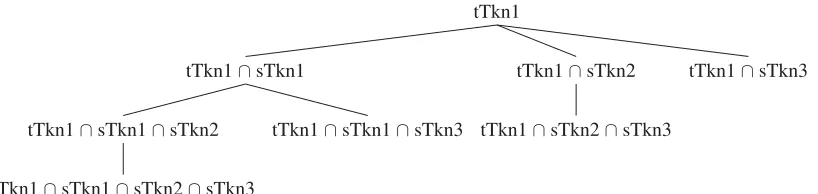
Figure 1: The root node of this tree represents an oversized block for the name Smith and the other nodes represent possible sub-blocks. The sub-blocking algorithm enumerates the tree breadth-first, stopping when it finds a correctly-sized sub-block.

in the tree is larger than or equal to any of its children. We traverse the tree breadth-first and only recurse into nodes above the maximum block size. This allows us to explore the space of possible sub-blocks in cardinality order for a given branch, stopping as soon as we have a small enough sub-block.

The algorithm that creates the blocks and sub-blocks takes as input a set of records and a maximum block size

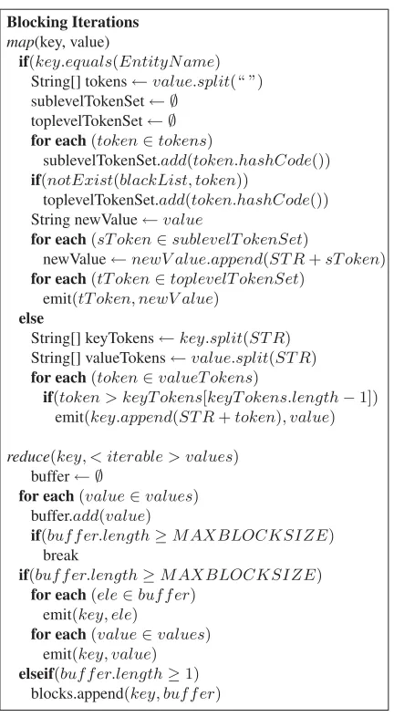
M. All the input records are grouped into blocks defined by the top-level properties. Those top-level blocks that are not above the maximum size are set aside. The re-maining oversized blocks are partitioned into sub-blocks by sub-blocking properties that the records they con-tain share, and those properties are appended to the key. The process is continued recursively until all sub-blocks have been whittled down to an acceptable size. The pseudo code of the blocking algorithm is presented in Figure 2. We will represent the key and value pairs in the MapReduce framework as < key;value >. The input organization records are represented as <

IN P U T F LAG, ORG N AM E >. For the first

iter-ation, this job takes the organization list as input. In later iterations, the input is the output of the previous blocking iteration. In the first iteration, the mapper function extracts the top-level and sub-level tokens from the input records. It combines the organization name and all the sub-level tokens in a temp variable called

newV alue. Next, for each top-level token, it emits this

top-level token and the newValue in the following

for-mat: < topT oken, newV alue >. For the later

itera-tions, it combines each sub level token with the current blocking key, and emits them to the reducer. Also note that the lexicographic ordering of the block keys allows separate mapper processes to work on different nodes in a level of the binomial tree without creating redundant sub-blocks (e.g. if one mapper creates a International∩ Busi-ness∩Machines block another mapper will not create a International∩Machines∩Business one). This is nec-essary because individual MapReduce jobs run indepen-dently without shared memory or other runtime commu-nication mechanisms. In the reduce phase, all the records will be grouped together for each block key. The reducer

function iterates over all the records in a newly-created sub-block, counting them to determine whether or not the block is small enough or needs to be further subdivided. The blocks that the reducer deems oversized become in-puts to the next iteration. Care is taken that the memory requirements of the reducer function are constant in the size of a fixed buffer because otherwise the reducer runs out of memory on large blocks. Note that we create a black list from the high frequency words in organization names, and we don’t use these as top-level properties as such words do not help us with individuating the records. More formally, this process can be understood in terms of operations on sets. In a set of N records there are

1

2N(N − 1) unique pairs, so an enumeration over all

of them isO(N2). The process of blocking divides this original set intokblocks, each of which contains at most a fixed maximum ofM records. The exhaustive compar-ison of pairs from these sets isO(k), and the constant factors are tractable if we choose a small enoughM. In the worst case, all the sub-blocks except the ones with the very longest keys are oversize. Then the sub-blocking al-gorithm will explore the powerset of all possible block-ing keys and thus have exponential runtime. However, as the blocking keys get longer, the sets they represent get smaller and eventually fall beneath the maximum size. In practice these two countervailing motions work to keep this strategy tractable.

2.2 Pairwise Linkage Model

In this section, we give just a brief overview of our pair-wise linkage system as a detailed description and evalua-tion of that system is beyond the scope of this paper.

We take a feature-based classification approach to pre-dict the likelihood of two organization names< o₁, o₂>

referring to the same organization entity. Specifically, we use the OpenNLP1maximum entropy (maxent) package as our machine learning tool. We choose to work with maxent because the training is fast and it has a good sup-port for classification. Regarding the features, we mainly have two types: surface string features and context fea-tures. Examples of surface string features are edit

Blocking Iterations

map(key, value)

if(key.equals(EntityN ame)

String[] tokens←value.split(“ ”)

sublevelTokenSet← ∅ toplevelTokenSet← ∅

for each(token∈tokens)

sublevelTokenSet.add(token.hashCode()) if(notExist(blackList, token))

toplevelTokenSet.add(token.hashCode())

String newValue←value

for each(sT oken∈sublevelT okenSet)

newValue←newV alue.append(ST R+sT oken) for each(tT oken∈toplevelT okenSet)

emit(tT oken, newV alue) else

String[] keyTokens←key.split(ST R)

String[] valueTokens←value.split(ST R) for each(token∈valueT okens)

if(token > keyT okens[keyT okens.length−1])

emit(key.append(ST R+token), value)

reduce(key, < iterable > values)

buffer← ∅

for each(value∈values)

buffer.add(value)

if(buf f er.length≥M AXBLOCKSIZE)

break

if(buf f er.length≥M AXBLOCKSIZE) for each(ele∈buf f er)

emit(key, ele)

for each(value∈values)

emit(key, value) elseif(buf f er.length≥1)

blocks.append(key, buf f er)

Figure 2: Alg.1 - Blocking

tance of the two names, whether one name is an abbre-viation of the other name, and the longest common sub-string of the two names. Examples of context features are whether the two names share the same url and the number of times that the two names co-occur with each other in a single person record.

2.3 Clustering

In this section, we present our clustering approach. Let’s, first clarify a set of terms/conditions that will help us de-scribe the algorithms.

Definition (Connected Component):Let G =(V, E)

be an undirected graph where V is the set of vertices and E is the set of edges. C =(C₁, C₂, ..., C_n)is the set of disjoint connected components in this graph where(C₁∪ C₂∪...∪C_n)= V and(C₁∩C₂∩...∩C_n)=∅. For each connected componentC_i∈C, there exists a path in G between any two verticesv_k andv_lwhere(v_k, v_l) ∈ C_i. Additionally, for any distinct connected component

sClust Transitive

Closure Edge List

Node - ClusterID mapping

anyClus ter > maxSize

no yes

Extract Pairs

Figure 3: Clustering Component

(C_i, C_j)∈ C, there is no path between any pairv_k and

v_lwherev_k ∈ C_i,v_l ∈ C_j. Moreover, the problem of finding all connected components in a graph is finding theCsatisfying the above conditions. Definition (Component ID): A component id is a unique identifier assigned to each connected component. Definition (Max Component Size): This is the maxi-mum allowed size for a connected component. Definition (Cluster Set): A cluster set is a set of records that belong to the same real world entity. Definition (Max Cluster Size):This is the maximum

allowed size for a cluster.

Definition (Match Threshold): Match threshold is a score where pairs scoring above this score are said to

rep-resent the same entity.

Definition (No-Match Threshold):No-Match thresh-old is a score where pairs scoring below this score are said

to represent different entities.

Definition (Conflict Set): Each record has a conflict set which is the set of records that shouldn’t appear with

this record in any of the clusters.

The naive approach to clustering for entity resolu-tion is transitive closure by using only the pairs having scores above the match threshold. However, in practice we might see many examples of conflicting scores. For example, (a,b) and (b,c) pairs might have scores above match threshold while (a,c) pair has a score below no-match threshold. If we just use transitive closure, we will end up with a single cluster with these three records (a,b,c). Another weakness of the regular transitive clo-sure is that it creates disjoint sets. However, organiza-tions might share name, or abbreviation. So, we need a soft clustering approach where a record might be in dif-ferent clusters.

par-TC-Iterate TC-Dedup Edge List

Node - ComponentID

mapping

newPair > 0

no yes

iterationID=1 iterationID>1

Figure 4: Transitive Closure Component

allelized clustering approaches with high precision for large scale graphs due to high time and space complexi-ties (Bansal, 2003). So, we propose a two-step approach in order to build both a parallel and an accurate clustering framework. The high-level architecture of our cluster-ing framework is illustrated in Figure 3. We first find the connected components in the graph with our MapReduce based transitive closure approach, then further, partition each connected component in parallel with our novel soft clustering algorithm, sClust. This way, we first combine similar record pairs into connected components in an effi-cient and scalable manner, and then further partition each connected component into smaller clusters for better pre-cision. Note that there is a dangerous phenomenon, black hole entities, in transitive closure of the pairwise scores (Michelson, 2009). A black hole entity begins to pull an inordinate amount of records from an increasing num-ber of different true entities into it as it is formed. This is dangerous, because it will then erroneously match on more and more records, escalating the problem. Thus, by the end of the transitive closure, one might end up with black hole entities with millions of records belonging to multiple different entities. In order to avoid this problem, we define a black hole threshold, and if we end up with a connected component above the size of the black hole threshold, we increment the match threshold by a delta and further partition this black hole with one more tran-sitive closure job. We repeat this process until the sizes of all the connected components are below the black hole threshold, and then apply sClust on each connected com-ponent. Hence at the end of the entire entity resolution process, the system has partitioned all the input records into cluster sets called profiles, where each profile corre-sponds to a single entity.

2.4 Transitive Closure

In order to find the connected components in a graph, we developed theTransitive Closure(TC) module shown in Figure 4. The input to the module is the list of all pairs having scores above the match threshold. As an output from the module, what we want to obtain is the mapping from each node in the graph to its corresponding com-ponentID. For simplicity, we use the smallest node id in each connected component as the identifier of that com-ponent. Thus, the module should output a mapping table from each node in the graph to the smallest node id in its corresponding connected component. To this end, we designed a chain of two MapReduce jobs, namely,

TC-Transitive Closure Iterate map(key, value)

emit(key, value)

emit(value, key)

reduce(key, < iterable > values)

minV alue←values.next()

if(minV alue < key)

emit(key, minV alue)

for each(value∈values)

Counter.NewPair.increment(1)

emit(value, minV alue)

(a) Transitive Closure - Iterate

Transitive Closure Dedup map(key, value)

emit(key.append(ST R+value), null)

reduce(key, < iterable > values)

String[] keyTokens←key.split(ST R)

emit(keyT okens[0], keyT okens[1])

(b) Transitive Closure - Dedup

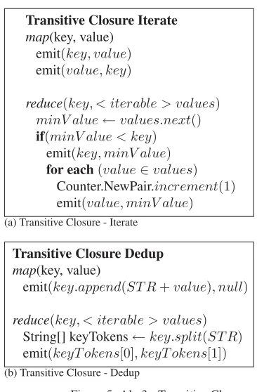
Figure 5: Alg.3 - Transitive Closure

Iterate, and TC-Dedup, that will run iteratively till we find the corresponding componentIDs for all the nodes in the graph.

TC-Iterate job generates adjacency lists AL =

(a₁, a₂, ..., a_n)for each nodev, and if the node id of this nodev_id is larger than the min node ida_minin the adja-cency list, it first creates a pair(v_id, a_min)and then a pair for each(a_i, a_min)wherea_i ∈AL, anda_i = a_min. If there is only one node inAL, it means we will generate the pair that we have in previous iteration. However, if there is more than one node inAL, it means we might generate a pair that we didn’t have in the previous itera-tion, and one more iteration is needed. Please note that, ifv_idis smaller thana_min, we don’t emit any pair.

The pseudo code of TC-Iterate is given in Figure 5-(a). For the first iteration, this job takes the pairs having scores above the match threshold from the initial edge list as input. In later iterations, the input is the output of TC-Dedup from the previous iteration. We first start with the initial edge list to construct the first degree neighborhood of each node. To this end, for each edge< a;b >, the mapper emits both< a;b >, and< b;a >pairs so that

Bring together all edges for each partition Phase-1

map(key, value)

if(key.equals(Conf lationOutput))

if((value.score≤N O M AT CH T HR)||

(value.score≥M AT CH T HR))

emit(value.entity1, value)

else //T CDedupOutput

temp.entity1←value

temp.entity2←null

temp.score←null

emit(key, temp)

emit(value, temp)

reduce(key, < iterable > values)

valueList← ∅

for each(value∈values)

if(value.entity2 =null)

clusID←value.entity1

else

valueList.add(value)

for each(value∈valueList)

emit(clusID, value)

Phase-2 map(key, value)

emit(key, value)

reduce(key, < iterable > values)

valueList← ∅

for each(value∈values)

valueList.add(value)

emit(key, valueList)

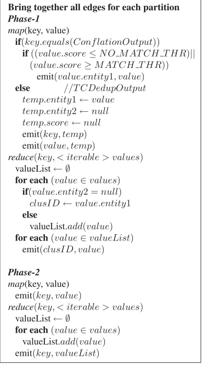
Figure 6: Alg.3 - Bring together all edges for each partition

we first emit the< key;minV alue > pair. Next, we emit a pair for all other values as< value;minV alue >, and increase the global NewPair counter by 1. If the counter is 0 at the end of the job, it means that we found all the components and there is no need for further itera-tions.

During the TC-Iterate job, the same pair might be emit-ted multiple times. The second job, TC-Dedup, just dedu-plicates the output of the CCF-Iterate job. This job in-creases the efficiency of TC-Iterate job in terms of both speed and I/O overhead. The pseudo code for this job is given in Figure 5-(b).

The worst case scenario for the number of necessary iterations is d+1 where d is the diameter of the net-work. The worst case happens when the min node in the largest connected component is an end-point of the largest shortest-path. The best case scenario takes d/2+1 iterations. For the best case, the min node should be at the center of the largest shortest-path.

2.5 sClust: A Soft Agglomerative Clustering Approach

After partitioning the records into disjoint connected components, we further partition each connected compo-nent into smaller clusters with sClust approach. sClust is a soft agglomerative clustering approach, and its main difference from any other hierarchical clustering method is the “conflict set” term that we described above. Any of the conflicting nodes cannot appear in a cluster with this approach. Additionally, the maximum size of the clusters can be controlled by an input parameter.

First as a preprocessing step, we have a two-step MapReduce job (see Figure 6) which puts together and sorts all the pairwise scores for each connected compo-nent discovered by transitive closure. Next, sClust job takes the sorted edge lists for each connected component as input, and partitions each connected component in par-allel. The pseudo-code for sClust job is given in Figure 7. sClust iterates over the pairwise scores twice. During the first iteration, it generates the node structures, and conflict sets for each of these structures. For example, if the pair-wise score for(a, b)pair is below the no-match threshold, nodeais added to nodeb’s conflict set, and vice versa. By the end of the first iteration, all the conflict sets are gen-erated. Now, one more pass is needed to build the final clusters. Since the scores are sorted, we start from the highest score to agglomeratively construct the clusters by going over all the scores above the match threshold. Let’s assume we have a pair(a, b)with a score above the match threshold. There might be 4 different conditions. First, both nodeaand nodebare not in any of the clusters yet. In this case, we generate a cluster with these two records and the conflict set of this cluster becomes the union of conflict sets of these two records. Second, nodeamight already be assigned to a set of clusters C’ while nodebis not in any of the clusters. In these case, we add nodebto each cluster in C’ if it doesn’t conflict withb. If there is no such cluster, we build a new cluster with nodesaand

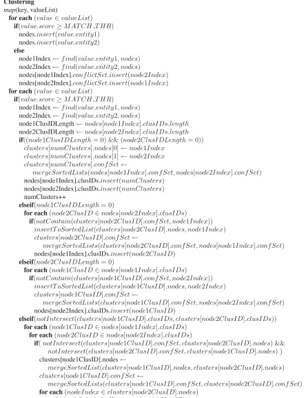
Clustering

map(key, valueList)

for each(value∈valueList)

if(value.score≥M AT CH T HR)

nodes.insert(value.entity1)

nodes.insert(value.entity2)

else

node1Index←f ind(value.entity1, nodes)

node2Index←f ind(value.entity2, nodes)

nodes[node1Index].conf lictSet.insert(node2Index)

nodes[node2Index].conf lictSet.insert(node1Index)

for each(value∈valueList)

if(value.score≥M AT CH T HR)

node1Index←f ind(value.entity1, nodes)

node2Index←f ind(value.entity2, nodes)

node1ClusIDLength←nodes[node1Index].clusIDs.length

node2ClusIDLength←nodes[node2Index].clusIDs.length

if((node1ClusIDLength= 0) && (node2ClusIDLength= 0))

clusters[numClusters].nodes[0]←node1Index

clusters[numClusters].nodes[1]←node2Index

clusters[numClusters].conf Set←

mergeSortedLists(nodes[node1Index].conf Set, nodes[node2Index].conf Set)

nodes[node1Index].clusIDs.insert(numClusters)

nodes[node2Index].clusIDs.insert(numClusters)

numClusters++

elseif(node1ClusIDLength= 0)

for each(node2ClusID∈nodes[node2Index].clusIDs)

if(notContain(clusters[node2ClusID].conf Set, node1Index))

insertT oSortedList(clusters[node2ClusID].nodes, node1Index)

clusters[node2ClusID].conf Set←

mergeSortedLists(clusters[node2ClusID].conf Set, nodes[node1Index].conf Set)

nodes[node1Index].clusIDs.insert(node2ClusID)

elseif(node2ClusIDLength= 0)

for each(node1ClusID∈nodes[node1Index].clusIDs)

if(notContain(clusters[node1ClusID].conf Set, node2Index))

insertT oSortedList(clusters[node1ClusID].nodes, node2Index)

clusters[node1ClusID].conf Set←

mergeSortedLists(clusters[node1ClusID].conf Set, nodes[node2Index].conf Set)

nodes[node2Index].clusIDs.insert(node1ClusID)

elseif(notIntersect(clusters[node1ClusID].clusIDs, clusters[node2ClusID].clusIDs))

for each(node1ClusID∈nodes[node1Index].clusIDs)

for each(node2ClusID∈nodes[node2Index].clusIDs)

if(notIntersect(clusters[node1ClusID].conf Set, clusters[node2ClusID].nodes) &&

notIntersect(clusters[node2ClusID].conf Set, clusters[node1ClusID].nodes) )

clusters[node1ClusID].nodes←

mergeSortedList(clusters[node1ClusID].nodes, clusters[node2ClusID].nodes)

clusters[node1ClusID].conf Set←

mergeSortedLists(clusters[node1ClusID].conf Set, clusters[node2ClusID].conf Set)

for each(nodeIndex∈clusters[node2ClusID].nodes)

nodes[nodeIndex].clusIDs.insert(node1ClusID)

clusters[node2ClusID].isRemoved←true

clusters[node2ClusID].nodes←null

clusters[node2ClusID].confSet←null

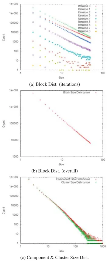
(a) Block Dist. (iterations)

(b) Block Dist. (overall)

(c) Component & Cluster Size Dist.

Figure 8: Size Distributions

3

Evaluation

In this section, we present the experimental results for our entity resolution framework. We ran the experiments on a hadoop cluster consisting of 50 nodes, each with 8 cores. There are 10 mappers, and 6 reducers available at each node. We also allocated 3 Gb memory for each map/reduce task.

We used two different real-world datasets for our ex-periments. The first one is a list of 150K organizations along with their aliases provided by freebase2. By using this dataset, we both trained our pairwise linkage model and measured the precision and recall of our system. We randomly selected 135K organizations from this list for the training. We used the rest of the organizations to

mea-2_{http://www.freebase.com/}

precision recall f-measure Pairwise Classifier 97 63 76 Transitive Closure 64 98 77

sClust 95 76 84

Table 1: Performance Comparison

sure the performance of our system. Next, we generated positive examples by exhaustively generating a pair be-tween all the aliases. We also randomly generated equal number of negative examples among pairs of different organization alias sets. We trained our pairwise classi-fier with the training set, then ran it on the test set and measured its performance. Next, we extracted all the or-ganization names from this set, and ran our entire entity resolution pipeline on top of this set. Table 1 presents the performance results. Our pairwise classifier has 97% precision and 63% recall when we use a match threshold of 0.65. Using same match threshold, we then performed transitive closure. We also measured the precision and recall numbers for transitive closure as it is the naive ap-proach for the entity resolution problem. Since transitive closure merges records transitively, it has very high recall but the precision is just 64%. Finally, we performed our sClust approach with the same match threshold. We set the no-match threshold to 0.3. The pairwise classifier has slightly better precision than sClust but sClust has much better recall. Overall, sClust has a much better f-measure than both the pairwise classifier and transitive closure.

Second, we used our production set to show the viabil-ity of our framework. In this set, we have 68M organiza-tion names. We ran our framework on this dataset. Block-ing generated 14M unique blocks, and there are 842M unique comparisons in these blocks. The distribution of the block sizes presented in Figure 8-(a) and (b). Block-ing finished in 42 minutes. Next, we ran our pairwise classifier on these 842M pairs and it finished in 220 min-utes. Finally, we ended up with 10M clusters at the end of the clustering stage which took 3 hours. The distribu-tion of the connected components and final clusters are presented in Figure 8-(c).

4

Conclusion

References

A. K. Elmagarmid, P. G. Iperirotis, and V. S. Verykios. Dupli-cate record detection: A survey. InIEEE Transactions on

Knowledge and Data Engineering, pages 1–16, 2007.

J. Lin and C. Dyer. Data-Intensive Text Processing with

MapReduce. Synthesis Lectures on Human Langugage

Technologies. Morgan & Claypool, 2010.

N. Bansal, A. Blum and S. Chawla Correlation Clustering.

Ma-chine Learning, 2003.

M. Michelson and S.A. Macskassy Record Linkage Measures in an Entity Centric World. In Proceedings of the 4th

work-shop on Evaluation Methods for Machine Learning,

Mon-treal, Canada, 2009.

N. Adly. Efficient record linkage using a double embedding scheme. In R. Stahlbock, S. F. Crone, and S. Lessmann, edi-tors,DMIN, pages 274–281. CSREA Press, 2009.

A. N. Aizawa and K. Oyama. A fast linkage detection scheme for multi-source information integration. InWIRI, pages 30– 39. IEEE Computer Society, 2005.

R. Baxter, P. Christen, and T. Churches. A comparison of fast blocking methods for record linkage, 2003.

M. Bilenko and B. Kamath. Adaptive blocking: Learning to scale up record linkage. InData Mining, 2006. ICDM’, num-ber Decemnum-ber, 2006.

P. Christen. A survey of indexing techniques for scalable record linkage and deduplication. IEEE Transactions on

Knowl-edge and Data Engineering, 99(PrePrints), 2011.

T. de Vries, H. Ke, S. Chawla, and P. Christen. Robust record linkage blocking using suffix arrays. InProceedings of the 18th ACM conference on Information and knowledge

man-agement, CIKM ’09, pages 305–314, New York, NY, USA,

2009. ACM.

T. de Vries, H. Ke, S. Chawla, and P. Christen. Robust record linkage blocking using suffix arrays and bloom filters. ACM

Trans. Knowl. Discov. Data, 5(2):9:1–9:27, Feb. 2011.

M. A. Hernandez and S. J. Stolfo. Real-world data is dirty. data cleansing and the merge/purge problem. Journal of Data

Mining and Knowledge Discovery, pages 1–39, 1998.

L. Jin, C. Li, and S. Mehrotra. Efficient record linkage in large data sets. InProceedings of the Eighth International

Confer-ence on Database Systems for Advanced Applications,

DAS-FAA ’03, pages 137–, Washington, DC, USA, 2003. IEEE Computer Society.

A. McCallum, K. Nigam, and L. H. Ungar. Efficient clustering of high-dimensional data sets with application to reference matching. InProceedings of the ACM International

Confer-ence on Knowledge Discover and Data Mining, pages 169–

178, 2000.

J. Nin, V. Muntes-Mulero, N. Martinez-Bazan, and J.-L. Larriba-Pey. On the use of semantic blocking techniques for data cleansing and integration. InProceedings of the 11th International Database Engineering and Applications

Sym-posium, IDEAS ’07, pages 190–198, Washington, DC, USA,

2007. IEEE Computer Society.

A. D. Sarma, A. Jain, and A. Machanavajjhala. CBLOCK: An Automatic Blocking Mechanism for Large-Scale De-duplication Tasks. Technical report, 2011.

M. Weis, F. Naumann, U. Jehle, J. Lufter, and H. Schuster. Industry-scale duplicate detection. Proc. VLDB Endow., 1(2):1253–1264, Aug. 2008.

S. E. Whang, D. Menestrina, G. Koutrika, M. Theobald, and H. Garcia-Molina. Entity resolution with iterative blocking.

InProceedings of the 35th SIGMOD international

confer-ence on Management of data, SIGMOD ’09, pages 219–232,

New York, NY, USA, 2009. ACM.

W. Winkler. Overview of record linkage and current research directions. Technical report, U.S. Bureau of the Census, 2006.

S. Yan, D. Lee, M.-Y. Kan, and L. C. Giles. Adaptive sorted neighborhood methods for efficient record linkage. In Pro-ceedings of the 7th ACM/IEEE-CS joint conference on

Dig-ital libraries, JCDL ’07, pages 185–194, New York, NY,

USA, 2007. ACM.

L. Kolb, and E. Rahm. Parallel entity resolution with Dedoop. Datenbank-Spektrum (2013): 1-10.