Proceedings of the NAACL HLT Workshop on Unsupervised and Minimally Supervised Learning of Lexical Semantics, pages 36–44,
Graph Connectivity Measures for Unsupervised Parameter Tuning
of Graph-Based Sense Induction Systems
Ioannis Korkontzelos, Ioannis Klapaftis and Suresh Manandhar Department of Computer Science
The University of York Heslington, York, YO10 5NG, UK
{johnkork, giannis, suresh}@cs.york.ac.uk
Abstract
Word Sense Induction (WSI) is the task of identifying the different senses (uses) of a tar-get word in a given text. This paper focuses on the unsupervised estimation of the free pa-rameters of a graph-based WSI method, and explores the use of eight Graph Connectiv-ity Measures (GCM) that assess the degree of connectivity in a graph. Given a target word and a set of parameters, GCM evaluate the connectivity of the produced clusters, which correspond to subgraphs of the initial (unclus-tered) graph. Each parameter setting is as-signed a score according to one of the GCM and the highest scoring setting is then selected. Our evaluation on the nouns of SemEval-2007 WSI task (SWSI) shows that: (1) all GCM es-timate a set of parameters which significantly outperform the worst performing parameter setting in both SWSI evaluation schemes, (2) all GCM estimate a set of parameters which outperform the Most Frequent Sense (MFS) baseline by a statistically significant amount in the supervised evaluation scheme, and (3) two of the measures estimate a set of ters that performs closely to a set of parame-ters estimated in supervised manner.
1 Introduction
Using word senses instead of word forms is essential in many applications such as information retrieval (IR) and machine translation (MT) (Pantel and Lin, 2002). Word senses are a prerequisite for word sense disambiguation (WSD) algorithms. However, they are usually represented as a fixed-list of definitions of a manually constructed lexical database. The
fixed-list of senses paradigm has several disadvan-tages. Firstly, lexical databases often contain general definitions and miss many domain specific senses (Agirre et al., 2001). Secondly, they suffer from the lack of explicit semantic and topical relations be-tween concepts (Agirre et al., 2001). Thirdly, they often do not reflect the exact content of the context in which the target word appears (Veronis, 2004). WSI aims to overcome these limitations of hand-constructed lexicons.
Most WSI systems are based on the vector-space model that represents each context of a target word as a vector of features (e.g. frequency of cooccur-ring words). Vectors are clustered and the resulting clusters are taken to represent the induced senses. Recently, graph-based methods have been employed to WSI (Dorow and Widdows, 2003; Veronis, 2004; Agirre and Soroa, 2007b).
Typically, graph-based approaches represent each word co-occurring with the target word, within a pre-specified window, as a vertex. Two vertices are connected via an edge if they co-occur in one or more contexts of the target word. This co-occurrence graph is then clustered employing differ-ent graph clustering algorithms to induce the senses. Each cluster (induced sense) consists of words ex-pected to be topically related to the particular sense. As a result, graph-based approaches assume that each context word is related to one and only one sense of the target one.
posed the use of a graph-based model for WSI, in which each vertex of the graph corresponds to a collocation (word-pair) that co-occurs with the tar-get word, while edges are drawn based on the co-occurrence frequency of their associated colloca-tions. Clustering of this collocational graph would produce clusters, which consist of a set of collo-cations. The intuition is that the produced clusters will be less sense-conflating than those produced by other graph-based approaches, since collocations provide strong and consistent clues to the senses of a target word (Yarowsky, 1995).
The collocational graph-based approach as well as the majority of state-of-the-art WSI systems es-timate their parameters either empirically or by em-ploying supervised techniques. The SemEval-2007 WSI task (SWSI) participating systems UOY and UBC-ASused labeled data for parameter estimation (Agirre and Soroa, 2007a), while the authors ofI2R, UPV SI andUMND2 have empirically chosen val-ues for their parameters. This issue imposes limits on the unsupervised nature of these algorithms, as well as on their performance on different datasets.
More specifically, when applying an unsupervised WSI system on different datasets, one cannot be sure that the same set of parameters is appropriate for all datasets (Karakos et al., 2007). In most cases, a new parameter tuning might be necessary. Unsupervised estimation of free parameters may enhance the unsu-pervised nature of systems, making them applicable to any dataset, even if there are no tagged data avail-able.
In this paper, we focus on estimating the free parameters of the collocational graph-based WSI method (Klapaftis and Manandhar, 2008) using eight graph connectivity measures (GCM). Given a parameter setting and the associated induced cluster-ing solution, each induced cluster corresponds to a subgraph of the original unclustered graph. A graph connectivity measureGCMi scores each cluster by
evaluating the degree of connectivity of its corre-sponding subgraph. Each clustering solution is then assigned the average of the scores of its clusters. Fi-nally, the highest scoring solution is selected.
Our evaluation on the nouns of SWSI shows that GCM improve the worst performing parame-ter setting by large margins in both SWSI evaluation schemes, although they are below the best
perform-ing parameter settperform-ing. Moreover, the evaluation in a WSD setting shows that all GCM estimate a set of parameters which are above the Most Frequent Sense (MFS) baseline by a statistically significant amount. Finally our results show that two of the measures, i.e. average degree and weighted average degree, estimate a set of parameters that performs closely to a set of parameters estimated in a super-vised manner. All of these findings, suggest that GCM are able to identify useful differences regard-ing the quality of the induced clusters for different parameter combinations, in effect being useful for unsupervised parameter estimation.
2 Collocational graphs for WSI
Letbc, be the base corpus, which consists of para-graphs containing the target word tw. The aim is to induce the senses of twgivenbc as the only in-put. Letrcbe a large reference corpus. In Klapaftis and Manandhar (2008) the British National Corpus1
is used as a reference corpus. The WSI algorithm consists of the following stages.
Corpus pre-processing The target of this stage is to filter the paragraphs of the base corpus, in order to keep the words which are topically (and possibly se-mantically) related to the target one. Initially,twis removed frombcand bothbcandrcare PoS-tagged. In the next step, only nouns are kept in the para-graphs ofbc, since they are characterised by higher discriminative ability than verbs, adverbs or adjec-tives which may appear in a variety of different con-texts. At the end of this pre-processing step, each paragraph ofbcandrcis a list of lemmatized nouns (Klapaftis and Manandhar, 2008).
In the next step, the paragraphs of bc are fil-tered by removing common nouns which are noisy; contextually not related to tw. Given a contex-tual wordcw that occurs in the paragraphs ofbc, a log-likelihood ratio (G2) test is employed (Dunning, 1993), which checks if the distribution ofcw inbc is similar to the distribution ofcwinrc;p(cw|bc) = p(cw|rc)(null hypothesis). If this is true,G2 has a small value. If this value is less than a pre-specified threshold (parameterp1) the noun is removed from bc.
Target:cnn nbc Target:nbc news
nbc tv nbc tv
cnn tv soap opera cnn radio nbc show
news newscast news newscast
radio television nbc newshour
cnn headline cnn headline
nbc politics radio tv
[image:3.612.113.258.70.175.2]breaking news breaking news
Table 1: Collocations connected tocnn nbcandnbc news
This process identifies nouns that are more indica-tive inbcthan inrcand vice versa. However, in this setting we are not interested in nouns which have a distinctive frequency in rc. As a result, eachcw which has a relative frequency inbcless than inrc is filtered out. At the end of this stage, each para-graph ofbcis a list of nouns which are assumed to be contextually related to the target wordtw.
Creating the initial collocational graph The tar-get of this stage is to determine the related nouns, which will form the collocations, and the weight of each collocation. Klapaftis and Manandhar (2008) consider collocations of size 2, i.e. pairs of nouns.
For each paragraph of bc of sizen, collocations are identified by generating all the possible cn
2
combinations. The frequency of a collocation c is the number of paragraphs in the whole SWSI corpus (27132 paragraphs), in whichcoccurs.
Each collocation is assigned a weight, measuring the relative frequency of two nouns co-occurring. Let f reqij denote the number of paragraphs in
which nounsiandj cooccur, andf reqj denote the
number of paragraphs, where noun j occurs. The conditional probabilityp(i|j)is defined in equation 1, and p(j|i) is computed in a similar way. The weight of collocationcij is the average of these
con-ditional probabilitieswcij =p(i|j) +p(j|i).
p(i|j) = f reqij
f reqj (1)
Finally, Klapaftis and Manandhar (2008) only ex-tract collocations which have frequency (parame-ter p2) and weight (parameter p3) higher than pre-specified thresholds. This filtering appears to com-pensate for inaccuracies in G2, as well as for low-frequency distant collocations that are ambiguous. Each weighted collocation is represented as a
ver-tex. Two vertices share an edge, if they co-occur in one or more paragraphs ofbc.
Populating and weighing the collocational graph
The constructed graph, G, is sparse, since the pre-vious stage attempted to identify rare events, i.e. co-occurring collocations. To address this problem, Klapaftis and Manandhar (2008) apply a smooth-ing technique, similar to the one in Cimiano et al. (2005), extending the principle that a word is characterised by the company it keeps(Firth, 1957) to collocations. The target is to discover new edges between vertices and to assign weights to all edges.
Each vertex i (collocation ci) is associated to
a vector V Ci containing its neighbouring vertices
(collocations). Table 1 shows an example of two vertices, cnn nbcand nbc news, which are discon-nected inGof the target wordnetwork. The example was taken from Klapaftis and Manandhar (2008).
In the next step, the similarity between all vertex vectorsV CiandV Cjis calculated using the Jaccard
coefficient, i.e. JC(V Ci, V Cj) = ||V CV Cii∪∩V CV Cjj||. Two
collocationsciandcjare mutually similar ifciis the
most similar collocation tocj and vice versa.
Given that collocations ci and cj are mutually
similar, an occurrence of a collocationck with one
ofci, cj is also counted as an occurrence with the
other collocation. For example in Table 1, ifcnn nbc and nbc news are mutually similar, then the zero-frequency event between nbc news and cnn tv is set equal to the joint frequency between cnn nbc and cnn tv. Marginal frequencies of collocations are updated and the overall result is consequently a smoothing of relative frequencies.
The weight applied to each edge connecting ver-ticesiandj(collocationsciandcj) is the maximum
of their conditional probabilities: p(i|j) = f reqij
f reqj,
wheref reqiis the number of paragraphs collocation
cioccurs.p(j|i)is defined similarly.
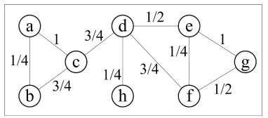
Figure 1: An example undirected weighted graph.
Initially, CW assigns all vertices to different classes. Each vertexiis processed for a number of iterations and inherits the strongest class in its lo-cal neighbourhood (LN) in an update step. LN is defined as the set of vertices which share an edge withi. In each iteration for vertexi: each class,cl, receives a score equal to the sum of the weights of edges (i,j), wherej has been assigned to classcl. The maximum score determines the strongest class. In case of multiple strongest classes, one is chosen randomly. Classes are updated immediately, mean-ing that a vertex can inherit from its LN classes that were introduced in the same iteration.
Once CW has produced the clusters of a target word, each of the instances of tw is tagged with one of the induced clusters. This process is simi-lar to Word Sense Disambiguation (WSD) with the difference that the sense repository has been auto-matically produced. Particularly, given an instance oftwin paragraphpi: each induced clusterclis
as-signed a score equal to the number of its collocations (i.e. pairs of words) occurring inpi. We observe that
the tagging method exploits the one sense per collo-cation property (Yarowsky, 1995), which means that WSD based on collocations is probably finer than WSD based on simple words, since ambiguity is re-duced (Klapaftis and Manandhar, 2008).
3 Unsupervised parameter tuning
In this section we investigate unsupervised ways to address the issue of choosing parameter values. To this end, we employ a variety of GCM, which mea-sure the relative importance of each vertex and as-sess the overall connectivity of the corresponding graph. These measures areaverage degree, cluster coefficient,graph entropyandedge density(Navigli and Lapata, 2007; Zesch and Gurevych, 2007).
GCM quantify the degree of connectivity of the produced clusters (subgraphs), which represent the
senses (uses) of the target word for a given cluster-ing solution (parameter settcluster-ing). Higher values of GCM indicate subgraphs (clusters) of higher con-nectivity. Given a parameter setting, the induced clustering solution and a graph connectivity measure GCMi, each induced cluster is assigned the
result-ing score of applyresult-ingGCMi on the corresponding
subgraph of the initial unclustered graph. Each clus-tering solution is assigned the average of the scores of its clusters (table 6), and the highest scoring one is selected.
For each measure, we have developed two ver-sions, i.e. one which considers the edge weights in the subgraph, and a second which does not. In the following description the terms graph and subgraph are interchangeable.
Let G = (V, E) be an undirected graph (in-duced sense), whereV is a set of vertices andE =
{(u, v) :u, v∈V}a set of edges connecting vertex pairs. Each edge is weighted by a positive weight, W :wuv→[0,∞). Figure 1 shows a small example
to explain the computation of GCM. The graph con-sists of 8 vertices,|V|= 8, and 10 edges,|E|= 10. Edge weights appear on edges, e.g.wab= 14.
Average Degree Thedegree (deg)of a vertexuis the number of edges connected tou:
deg(u) =|{(u, v)∈E:v∈V}| (2)
The average degree (AvgDeg) of a graph can be computed as:
AvgDeg(G(V, E)) = 1
|V|
X
u∈V
deg(u) (3)
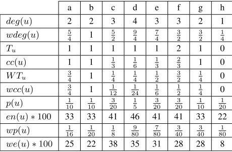
The first row of table 2 shows the vertex degrees of the example graph (figure 1) andAvgDeg(G) =
20 8 = 2.5.
Edge weights can be integrated into the degree computation. Let mew be the maximum edge weight in the graph:
mew= max
(u,v)∈Ewuv (4)
Average Weighted Degree The weighted de-gree(w deg)of a vertex is defined as:
w deg(u) = 1
|V|
X
(u,v)∈E
wuv
a b c d e f g h
deg(u) 2 2 3 4 3 3 2 1
wdeg(u) 5
4 1 5 2 9 4 7 4 3 2 3 2 1 4
Tu 1 1 1 1 1 2 1 0
cc(u) 1 1 13 16 13 23 1 0
W Tu 34 1 14 14 12 32 14 0
wcc(u) 3
4 1 1 12 1 24 1 6 1 2 1 4 0
p(u) 1
10 1 10 3 20 1 5 3 20 3 20 1 10 1 20
en(u)∗100 33 33 41 46 41 41 33 22
wp(u) 1
16 1 20 1 8 9 80 7 80 3 40 3 40 1 80
[image:5.612.72.302.72.223.2]we(u)∗100 25 22 38 35 31 28 28 8
Table 2: Computations of graph connectivity measures and relevant quantities on the example graph (figure 1).
Average weighted degree (AvgWDeg), similarly to AvgDeg, is averaged over all vertices of the graph. In the graph of figure 1,mew= 1. The second row of table 2 shows the weighted degrees of all vertices. AvgW Deg(G) = 4836 '1.33.
Average Cluster Coefficient The cluster coeffi-cient (cc)of a vertex,u, is defined as:
cc(u) = Tu
2−1k
u(ku−1) (6)
Tu =
X
(u,v)∈E
X
(v,x)∈E x6=u
1 (7)
Tu is the number of edges between the ku
neigh-bours ofu. Obviouslyku=deg(u).2−1ku(ku−1)
would be the number of edges between the neigh-bours of u if the graph they define was fully con-nected. Average cluster coefficient (AvgCC)is aver-aged over all vertices of the graph.
The computations ofTuandcc(u)on the example
graph are shown in the third and fourth rows of table 2. Consequently,AvgCC(G) = 169 = 0.5625.
Average Weighted Cluster Coefficient LetW Tu
be the sum of edge weights between the neighbours ofu overmew. Weighted cluster coefficient (wcc) can be computed as:
wcc(u) = W Tu
2−1k
u(ku−1) (8)
W Tu = 1
mew
X
(u,v)∈E
X
(v,x)∈E x6=u
wvx (9)
Average weighted cluster coefficient (AvgWCC) is averaged over all vertices of the graph. The com-putations ofW Tuandwcc(u)on the example graph
(figure 1) are shown in the fifth and sixth rows of table 2 andAvgW CC(G) = 867∗24 '0.349.
Graph Entropy Entropymeasures the amount of information (alternatively the uncertainty) in a ran-dom variable. For a graph, high entropy indicates that many vertices are equally important and low en-tropythat only few vertices are relevant (Navigli and Lapata, 2007). Theentropy (en)of a vertexucan be defined as:
en(u) =−p(u) log2p(u) (10)
The probability of a vertex, p(u), is determined by the degree distribution:
p(u) =
deg(u)
2|E|
u∈V
(11)
Graph entropy (GE) is computed by summing all vertex entropies and normalising bylog2|V|. The seventh and eighth row of table 2 show the compu-tations ofp(u)anden(u)on the example graph, re-spectively. Thus,GE'0.97.
Weighted Graph Entropy Similarly to previous graph connectivitymeasures, the weighted entropy (wen)of a vertexuis defined as:
we(u) =−wp(u) log2wp(u) (12)
where:wp(u) =
w deg(u)
2∗mew∗ |E|
u∈V
Weighted graph entropy (GE)is computed by sum-ming all vertex weighted entropies and normalising bylog2|V|. The last two rows of table 2 show the computations of wp(u) andwe(u) on the example graph. Consequently,W GE '0.73.
Edge Density and Weighted Edge Density Edge density (ed) quantifies how many edges the graph has, as a ratio over the number of edges of a fully connected graph of the same size:
A(V) = 2
|V|
2
Edge density (ed) is a global graph connectivity measure; it refers to the whole graph and not a spe-cific vertex. Edge density (ed) andweighted edge density (wed)can be defined as follows:
ed(G(V, E)) = |E|
A(V) (14)
wed(G(V, E)) = 1 A(V)
X
(u,v)∈E
wu,v
mew (15)
In the graph of figure 1: A(V) = 2 82 = 28, ed(G) = 1028 '0.357,P wu,v
mew = 6andwed(G) =
6
28 '0.214.
The use of the aforementioned GCM allows the estimation of a different parameter setting for each target word. Table 3 shows the parameters of the col-locational graph-based WSI system (Klapaftis and Manandhar, 2008). These parameters affect how the collocational graph is constructed, and in effect the quality of the induced clusters.
4 Evaluation
4.1 Experimental setting
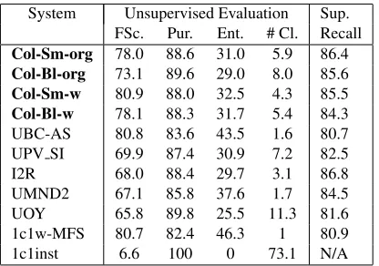
The collocational WSI approach was evaluated un-der the framework and corpus of SemEval-2007 WSI task (Agirre and Soroa, 2007a). The corpus consists of text of the Wall Street Journal corpus, and is hand-tagged with OntoNotes senses (Hovy et al., 2006). The evaluation focuses on all 35 nouns of SWSI. SWSI task employs two evaluation schemes. Inunsupervised evaluation, the results are treated as clusters of contexts and gold standard (GS) senses as classes. In a perfect clustering solution, each in-duced cluster contains the same contexts as one of the classes (Homogeneity), and each class contains the same contexts as one of the clusters ( Complete-ness). F-Score is used to assess the overall quality of clustering. Entropy and purity are also used, com-plementarily. F-Score is a better measure than en-tropy or purity, since F-Score measures both homo-geneity and completeness, while entropy and purity measure only the former. In the second scheme, su-pervised evaluation, the training corpus is used to map the induced clusters to GS senses. The testing corpus is then used to measure WSD performance (Table 4,Sup. Recall).
The graph-based collocational WSI method is re-ferred asCol-Sm (where “Col” stands for the
“col-Parameter Range Value
G2threshold 5, 10, 15 p 1= 5
Collocation frequency 4, 6, 8, 10 p2= 8
[image:6.612.328.525.71.116.2]Collocation weight 0.2, 0.3, 0.4 p3= 0.2
Table 3: Parameters ranges and values in Klapaftis and Manandhar (2008)
locational WSI” approach and “Sm” for its ver-sion using “smoothing”).Col-Bl(where “Bl” stands for “baseline”) refers to the same system without smoothing. The parameters ofCol-Sm were origi-nally estimated by cross-validation on the training set of SWSI. Out of 72 parameter combinations, the setting with the highest F-Score was chosen and ap-plied to all 35 nouns of the test set. This is referred asCol-Sm-org(where “org” stands for “original”) in Table 4. Table 3 shows all values for each parameter, and the chosen values, under supervised parameter estimation2. Col-Bl-org(Table 4) induces senses as
Col-Sm-orgdoes, but without smoothing.
In table 4, Col-Sm-w (respectively Col-Bl-w) refers to the evaluation ofCol-Sm(Col-Bl), follow-ing the same technique for parameter estimation as in Klapaftis and Manandhar (2008) for each target word separately (“w” stands for “word”). Given that GCM are applied for each target word separately, these baselines will allow to see the performance of GCM compared to a supervised setting.
The 1c1inst baseline assigns each instance to a distinct cluster, while the 1c1w baseline groups all instances of a target word into a single cluster. 1c1w is equivalent to MFS in this setting. The fifth column of table 4 shows the average number of clusters.
The SWSI participant systemsUOYandUBC-AS used labeled data for parameter estimation. The au-thors ofI2R,UPV SI andUMND2have empirically chosen values for their parameters.
The next subsection presents the evaluation of GCM as well as the results of SWSI systems. Ini-tially, we provide a brief discussion on the differ-ences between the two evaluation schemes of SWSI that will allow for a better understanding of GCM performance.
4.2 Analysis of results and discussion
System Unsupervised Evaluation Sup. FSc. Pur. Ent. # Cl. Recall
Col-Sm-org 78.0 88.6 31.0 5.9 86.4
Col-Bl-org 73.1 89.6 29.0 8.0 85.6
Col-Sm-w 80.9 88.0 32.5 4.3 85.5
Col-Bl-w 78.1 88.3 31.7 5.4 84.3 UBC-AS 80.8 83.6 43.5 1.6 80.7 UPV SI 69.9 87.4 30.9 7.2 82.5
I2R 68.0 88.4 29.7 3.1 86.8
UMND2 67.1 85.8 37.6 1.7 84.5 UOY 65.8 89.8 25.5 11.3 81.6 1c1w-MFS 80.7 82.4 46.3 1 80.9
[image:7.612.83.291.70.216.2]1c1inst 6.6 100 0 73.1 N/A
Table 4: Evaluation of WSI systems and baselines.
and entropy. However, F-Score of 1c1inst is low, because the GS senses are spread among clusters, decreasing unsupervised recall. Supervised recall of 1c1instis undefined, because each cluster tags only one instance. Hence, clusters tagging instances in the test corpus do not tag any instances in the train corpus and the mapping cannot be performed.1c1w achieves high F-Score due to the dominance of MFS in the testing corpus. However, its purity, entropy and supervised recall are much lower than other sys-tems, because it only induces the dominant sense.
Clustering solutions that achieve high supervised recall do not necessarily achieve high F-Score, mainly because F-Score penalises systems for in-ducing more clusters than the corresponding GS classes, as 1cl1inst does. Supervised evaluation seems to be more neutral regarding the number of clusters, since clusters are mapped into a weighted vector of senses. Thus, inducing a number of clus-ters similar to the number of senses is not a require-ment for good results (Agirre and Soroa, 2007a). High supervised recall means high purity and en-tropy, as inI2R, but not vice versa, as inUOY.UOY produces many clean clusters, however these are un-reliably mapped to senses due to insufficient train-ing data. On the contrary,I2Rproduces a few clean clusters, which are mapped more reliably.
Comparing the performance of SWSI systems shows that none performs well in both evaluation settings, in effect being biased against one of the schemes. However, this is not the case for the collo-cational WSI method, which achieves a high perfor-mance in both evaluation settings.
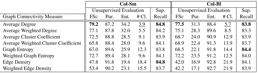
Table 6 presents the results of applying the graph
System Bound Unsupervised Evaluation Sup. type FSc. Pur. Ent. # Cl. Recall Col-Sm MaxR 79.3 90.5 26.6 7.0 88.6
Col-Sm MinR 62.9 89.0 26.7 12.7 78.8
Col-Bl MaxR 72.9 91.8 23.2 9.6 88.7
Col-Bl MinR 57.5 89.0 26.4 14.4 76.2
Col-Sm MaxF 83.2 90.0 28.7 4.9 86.6 Col-Sm MinF 43.6 90.2 22.1 17.6 83.7 Col-Bl MaxF 81.1 90.0 28.7 5.3 81.8 Col-Bl MinF 34.1 90.5 20.5 20.4 81.5
Table 5: Upper and lower performance bounds for sys-temsCol-SmandCol-Bl.
connectivity measures of section 3 in order to choose the parameter values for the collocational WSI sys-tem, for each word separately. The evaluation is done both forCol-SmandCol-Blthat use and ignore smoothing, respectively.
To evaluate the supervised recall performance using the graph connectivity measures, we com-puted both the upper and lower bounds ofCol-Sm, i.e. the best and worst supervised recall, respectively (MaxR and MinR in table 5). In the former case, we selected the parameter combination per target word that performs best (Col-Sm, MaxR in table 5), which resulted in 88.6% supervised recall (F-Score: 79.3%), while in the latter we selected the worst per-forming one, which resulted in 78.8% supervised re-call (F-Score: 62.9%). In table 6 we observe that the supervised recall of all measures is significantly lower than the upper bound. However, all measures perform significantly better than the lower bound (McNemar’s test, confidence level: 95%); the small-est difference is 4.9%, in the case of weighted edge density. The picture is the same forCol-Bl.
In the same vein, we computed both the upper and lower bounds ofCol-Smin terms of F-Score, 83.2% and 43.6%, respectively (Col-Sm, MinF and MaxF in table 5). The performance of the system is lower than the upper bound, for all GCM. Despite that, we observe that all measures except edge density and weighted edge density outperform the lower bound by large margins.
[image:7.612.315.541.70.185.2]Col-Sm Col-Bl
Unsupervised Evaluation Sup. Unsupervised Evaluation Sup. Graph Connectivity Measure FSc Pur. Ent. # Cl. Recall FSc Pur. Ent. # Cl. Recall
Average Degree 79.2 87.2 34.2 3.9 84.8 77.5 31.3 88.4 5.7 83.8
Average Weighted Degree 77.1 87.8 32.0 5.5 84.2 75.1 28.3 89.6 8.5 83.3 Average Cluster Coefficient 72.5 88.8 28.5 9.1 83.9 68.7 24.0 90.9 12.9 83.9 Average Weighted Cluster Coefficient 65.8 88.4 28.0 9.6 84.1 68.9 22.4 91.3 13.9 83.7
Graph Entropy 67.0 89.6 25.9 12.3 83.8 68.5 22.1 91.8 14.4 84.4
Weighted Graph Entropy 72.7 89.4 28.1 9.6 84.1 72.2 23.5 91.2 12.5 84.0
Edge Density 47.8 91.8 19.4 18.4 84.8 42.0 16.9 92.8 21.9 84.1
[image:8.612.84.532.70.197.2]Weighted Edge Density 53.4 90.2 23.1 15.5 83.7 42.2 17.1 92.7 21.9 83.9
Table 6: Unsupervised & supervised evaluation of the collocational WSI approach using graph connectivity measures.
case. However, they are all unable to approximate the upper bound for both evaluation schemes, which is also the case for the supervised estimation of pa-rameters per target word (Col-Sm-wandCol-Bl-w).
In Table 6, we also observe that all measures achieve higher supervised recall scores than the MFS baseline. The increase is statistically signif-icant (McNemar’s test, confidence level: 95%) in all cases. This result shows that irrespective of the number of clusters produced (low F-Score), GCM are able to estimate a set of parameters that provides clean clusters (low entropy), which when mapped to GS senses improve upon the most frequent heuristic, unlike the majority of unsupervised WSD systems.
Regarding the comparison between different GCM, we observe that average degree and weighted average degree for Col-Sm (Col-Bl) perform closely toCol-Sm-w(Col-Bl-w) for both evaluation schemes. This is due to the fact that they produce a number of clusters similar toCol-Sm-w(Col-Bl-w), while at the same time their distributions of clusters over the target words’ instances are also similar.
On the contrary, the remaining GCM tend to pro-duce larger numbers of clusters compared to both Col-Sm-w (Col-Bl-w) and the GS, in effect being penalised by F-Score. As it has already been men-tioned, supervised recall is less affected by a large number of clusters, which causes small differences among GCM.
Determining whether the weighted or unweighted version of GCM performs better depends on the GCM itself. Weighted graph entropy performs in all cases better than the unweighted version. For aver-age cluster coefficient and edge density, we cannot extract a safe conclusion. Unweighted average de-gree performs better than the weighted version.
5 Conclusion and future work
In this paper, we explored the use of eight graph con-nectivity measures for unsupervised estimation of free parameters of a collocational graph-based WSI system. Given a parameter setting and the associ-ated induced clustering solution, each cluster was scored according to the connectivity degree of its corresponding subgraph, as assessed by a particular graph connectivity measure. Each clustering solu-tion was then assigned the average of its clusters’ scores, and the highest scoring one was selected.
Evaluation on the nouns of SemEval-2007 WSI task (SWSI) showed that all eight graph connectiv-ity measures choose parameters for which the corre-sponding performance of the system is significantly higher than the lower performance bound, for both the supervised and unsupervised evaluation scheme. Moreover, the selected parameters produce results which outperform the MFS baseline by a statisti-cally significant amount in the supervised evalua-tion scheme. The best performing measures, average degree and weighted average degree, perform com-parably well to the set of parameters chosen by a supervised parameter estimation. In general, graph connectivity measures can quantify significant dif-ferences regarding the degree of connectivity of in-duced clusters.
References
Eneko Agirre and Aitor Soroa. 2007a. Semeval-2007 task 02: Evaluating word sense induction and discrim-ination systems. InProceedings of the Fourth Interna-tional Workshop on Semantic Evaluations (SemEval-2007), pages 7–12, Prague, Czech Republic. Associa-tion for ComputaAssocia-tional Linguistics.
Eneko Agirre and Aitor Soroa. 2007b. Ubc-as: A graph based unsupervised system for induction and classi-fication. In Proceedings of the Fourth International Workshop on Semantic Evaluations (SemEval-2007), pages 346–349, Prague, Czech Republic. Association for Computational Linguistics.
Eneko Agirre, Olatz Ansa, Eduard Hovy, and David Mar-tinez. 2001. Enriching wordnet concepts with topic signatures, Sep.
Chris Biemann. 2006. Chinese whispers - an efficient graph clustering algorithm and its application to nat-ural language processing problems. In Proceedings of TextGraphs: the Second Workshop on Graph Based Methods for Natural Language Processing, pages 73– 80, New York City, June. Association for Computa-tional Linguistics.
Philipp Cimiano, Andreas Hotho, and Steffen Staab. 2005. Learning concept hierarchies from text corpora using formal concept analysis. Journal of Artificial In-telligence research, 24:305–339.
Beate Dorow and Dominic Widdows. 2003. Discover-ing corpusspecific word senses. In Proceedings 10th conference of the European chapter of the ACL, pages 79–82, Budapest, Hungary.
Ted E. Dunning. 1993. Accurate methods for the statis-tics of surprise and coincidence. Computational Lin-guistics, 19(1):61–74.
John R. Firth. 1957. A synopsis of linguistic theory, 1930-1955. Studies in Linguistic Analysis, pages 1– 32.
Eduard Hovy, Mitchell Marcus, Martha Palmer, Lance Ramshaw, and Ralph Weischedel. 2006. Ontonotes: The 90% solution. InProceedings of the Human Lan-guage Technology Conference of the NAACL, Com-panion Volume: Short Papers, pages 57–60, New York City, USA. Association for Computational Linguistics. Damianos Karakos, Jason Eisner, Sanjeev Khudanpur, and Carey Priebe. 2007. Cross-instance tuning of un-supervised document clustering algorithms. InHuman Language Technologies 2007: The Conference of the North American Chapter of the Association for Com-putational Linguistics; Proceedings of the Main Con-ference, pages 252–259, Rochester, New York, April. Association for Computational Linguistics.
Ioannis P. Klapaftis and Suresh Manandhar. 2008. Word sense induction using graphs of collocations. In In
Proceedings of the 18th European Conference on Ar-tificial Intelligence, (ECAI-2008), Patras, Greece. R. Navigli and M. Lapata. 2007. Graph
connectiv-ity measures for unsupervised word sense disambigua-tion. In20th International Joint Conference on Artifi-cial Intelligence (IJCAI 2007), pages 1683–1688, Hy-derabad, India, January.
Patrick Pantel and Dekang Lin. 2002. Discovering word senses from text. In KDD ’02: Proceedings of the eighth ACM SIGKDD international conference on Knowledge discovery and data mining, pages 613– 619, New York, NY, USA. ACM Press.
Jean Veronis. 2004. Hyperlex: lexical cartography for information retrieval. Computer Speech & Language, 18(3):223–252, July.
David Yarowsky. 1995. Unsupervised word sense disam-biguation rivaling supervised methods. InMeeting of the Association for Computational Linguistics, pages 189–196.
Torsten Zesch and Iryna Gurevych. 2007. Analysis of the wikipedia category graph for NLP applications. In