Using Pseudowords for Algorithm Comparison: An Evaluation Framework for Graph based Word Sense Induction

Using Pseudowords for Algorithm Comparison:

An Evaluation Framework for Graph-based Word Sense Induction

DISCo

Universit`a degli Studi di Milano-Bicocca

[email protected]

Martin Riedl, Chris Biemann

Language Technology Group Universit¨at Hamburg

[email protected] [email protected]

Abstract

In this paper we define two parallel data sets based on pseudowords, extracted from the same corpus. They both consist of word-centered graphs for each of 1225 dif-ferent pseudowords, and use respectively first-order co-occurrences and second-order semantic similarities. We propose an evaluation framework on these data sets for graph-based Word Sense Induc-tion (WSI) focused on the case of coarse-grained homonymy: We compare differ-entWSI clustering algorithms by measur-ing how well their outputs agree with thea prioriknown ground-truth decomposition of a pseudoword. We perform this eval-uation for four different clustering algo-rithms: the Markov cluster algorithm, Chi-nese Whispers, MaxMax and a gangplank-based clustering algorithm. To further im-prove the comparison between these algo-rithms and the analysis of their behaviours, we also define a new specific evaluation measure. As far as we know, this is the first large-scale systematic pseudoword evalu-ation dedicated to the induction of coarse-grained homonymous word senses.

1 Introduction and Related Work

Word Sense Induction (WSI) is the branch of Natu-ral Language Processing (NLP) concerned with the unsupervised detection of all the possible senses that a term can assume in a text document. It could also be described as “unsupervised Word Sense Disambiguation” (Navigli, 2009). Since ambigu-ity and arbitrariness are constantly present in nat-ural languages,WSIcan help improve the analysis and understanding of text or speech (Martin and Jurafsky, 2000). At its core we find the notion of distributional semantics, exemplified by the

state-ment by Harris (1954): “Difference of meaning correlates with difference of distribution.”

In this paper, we focus on graph-based methods. Graphs provide an intuitive mathematical repre-sentation of relations between words. A graph can be defined and built in a straightforward way, but allows for a very deep analysis of its structural properties. This and their discrete nature (contrary to the continuous generalizations represented by vector spaces of semantics, cf. Turney and Pan-tel (2010)) favour the identification of significa-tive patterns and subregions, among other things allowing the final number of clusters to be left un-predetermined, an ideal condition forWSI.

The main contribution of this paper is three-fold: We present two parallel word graph data sets based on the concept of pseudowords, both for the case of semantic similarities and co-occurrences; on them, we compare the performances of four WSI clustering algorithms; and we define a new

ad hoc evaluation measure for this task, called TOP2.

Pseudowords were first proposed by Gale et al. (1992) and Sch¨utze (1992) as a way to cre-ate artificial ambiguous words by merging two (or more) random words. A pseudoword simulates homonymy, i.e. a word which possesses two (or more) semantically and etymologically unrelated senses, such ascountas “nobleman” as opposed to “the action of enumerating”. The study of Nakov and Hearst (2003) shows that the performances ofWSIalgorithms on random pseudowords might represent an optimistic upper bound with respect to true polysemous words, as generic polysemy implies some kind of correlation between the cate-gories and the distributions of the different senses of a word, which is absent from randomly gener-ated ones. We are aware of the approaches pro-posed in (Otrusina and Smrˇz, 2010) and (Pile-hvar and Navigli, 2013), used e.g. in (Bas¸kaya

and Jurgens, 2016), for a pseudoword generation that better models polysemous words with an ar-bitrary degree of polysemy. Both works imply the emulation of existing polysemous words, fol-lowing the semantic structure of WordNet (Miller, 1995): pseudosenses(the components of a pseu-doword) corresponding to the synsets of a word are represented by the closest monosemous terms on the WordNet graph, according to Personal-ized PageRank (Haveliwala, 2002) applied to the WordNet graph. However, we want to remark the different nature of our paper. Here we compare the behaviours of different clustering algorithms on two data sets of pseudowords built to emu-late homonymy, and reemu-late these behaviours to the structure of the word graphs relative to these pseu-dowords. As homonymy is more clear-cut than generic polysemy, we deem that the efficacy of a WSIalgorithm should be first measured in this case before being tested in a more fine-grained and am-biguous situation. Also, the task we defined does not depend on the arbitrary granularity of an ex-ternal lexical resource1_{, which might be too}

fine-grained for our purpose. Further, the sense distinc-tions e.g. in WordNet might not be mirrored in the corpus, and conversely, some unforeseen senses might be observed. Instead, our work can be seen as an expansion of the pseudoword evaluation pre-sented in (Bordag, 2006), albeit more focused in its goal and implementation.

In our opinion, current WSI tasks present some shortcomings. A fundamental problem is the vagueness regarding the granularity (fine or coarse) of the senses that have to be determined. As a consequence, the definition of an adequate evaluation measure becomes difficult, as many of them have been showed to be biased towards few or many clusters2_{. Further, small data sets often}

do not allow obtaining significant results. Pseu-doword evaluation, on the contrary, presents an objective and self-contained framework where the classification task is well characterized and gives the opportunity to define an ad hoc evaluation measure, at the same time automating the data set creation. Therefore, we tackle the following research questions: What are the limitations of a

1_{As was also the case for task 13 of SemEval 2013, cf.} (Jurgens and Klapaftis, 2013)

2_{See for example the results at task 14 of SemEval 2010} (Manandhar et al., 2010), where adjusted mutual information was introduced to correct the bias:https://www.cs.york. ac.uk/semeval2010_WSI/task_14_ranking.html.

pseudoword evaluation for homonymy detection? How does the structure of a pseudoword’s word graph depend on its components? How do dif-ferent clustering strategies compare on the same data set, and what are the most suited measures to evaluate their performances?

The paper is structured as follows. In Section 2 we give a definition of the ego word graph of a word and present our starting corpus. Section 3 details our evaluation setting and describes our proposed measureTOP2. Section 4 introduces the four graph clustering algorithms chosen for eval-uation. Lastly, Section 5 comments the results of the comparisons, and Section 6 concludes the pa-per.

2 Word Graphs and Data Set

For our evaluation we will use word graphs based both on semantic similarities (SSIM) and on co-occurrences. We define both as undirected, weighted graphs G= (V,E) whose nodes corre-spond to a given subset V of the vocabulary of the considered corpus, and where two nodesv,w are connected by an edge if and only if v andw co-occur in the same sentence (co-occurrences) or share some kind of context (semantic similarities). In either case, we express the strength of the con-nection between two words through a weight map-ping p:E−→R+_{, for which we can take} indica-tors such as raw frequency or pointwise mutual in-formation. The higher the value on an edge, the more significant we deem their connection. We will consider word-centered graphs, calledego word graphs. Both kinds of ego word graphs will be induced by the distributional thesauri com-puted on a corpus consisting of 105 million En-glish newspaper sentences3_{, using the JoBimText}

(Biemann and Riedl, 2013) implementation. In the case of co-occurrences, for a given wordvwe use a frequency-weighted version of pointwise mutual information called lexicographer’s mutual infor-mation(LMI) (Kilgarriff et al., 2004; Evert, 2004) to rank all the terms co-occurring withvin a sen-tence and to select those that will appear in its ego word graph. Edge weights are defined byLMIand the possible edge between two nodesuandwwill be determined by the presence ofuin the

tional thesaurus ofw, or viceversa.

The process is similar in the case of SSIMs, but here LMI is computed on term-context co-occurrences based on syntactic dependencies ex-tracted from the corpus by means of the Stanford Parser (De Marneffe et al., 2006).

In both cases, the wordvitself is removed from G, since we are interested just in the relations between the words more similar to it, following (Widdows and Dorow, 2002). The clusters in which the node set of G will be subdivided will represent the possible senses ofv. We remark that co-occurrences are first-order relations (i.e. in-ferred directly by data), whereasSSIMs are of sec-ond order, as they are computed on the base of co-occurrences4_{. For this reason, two different kinds}

of distributional thesauri might have quite differ-ent differ-entries even if they pertain to the same word. Further, the ensuing word graphs will show a com-plementary correlation: co-occurrences represent syntagmaticrelations with the central word, while SSIMs paradigmatic ones5, and this also deter-mines different structures, as e.g. co-occurrences are denser thanSSIMs.

3 Pseudoword Evaluation Framework

The method of pseudoword evaluation was first independently proposed in (Gale et al., 1992) and (Sch¨utze, 1992). Given two words appearing in a corpus, e.g. catandwindow, we replace all their occurrences therein with an artificial term formed by their combination (represented in our example as cat window), a so-called pseudoword that merges the contexts of its components (also called pseudosenses). The original application of this evaluation assumes that all the components of a pseudoword are monosemous words, i.e. possess only one sense. Ideally, an algorithm trying to induce the senses of a monosemous word from the corresponding word graph should return only one cluster, and we would expect it to find exactly two clusters in the case of a pseudoword with two components. This makes evaluation more transparent, and we are restricting ourselves to monosemous words for this reason.

For the purpose of our evaluation, we ex-tract monosemous nouns from the 105 million

4_{About relations of second and higher orders, cf.} (Bie-mann and Quasthoff, 2009).

5_{A fundamental source on this topic is (De Saussure, 1995} 1916).

sentences of the corpus described in Section 2, over which we compute all SSIM- and co-occurrence-based distributional thesauri. We divide all the nouns into 5 logarithmic frequency classes identified with respect to the frequency of the most common noun in the corpus. For each class, we extract random candidates: We retain only those that possess one single meaning, i.e. for which Chinese Whispers (see Section 4.2)6

yields one single cluster, additionally checking that they have only onesynsetin WordNet (which is commonly accepted to be fine-grained). We repeat this process until we obtain 10 suitable candidates per frequency class. In the end, we obtain a total of 50 words whose combinations give rise to 1225 different pseudowords. We then proceed to create two kinds of pseudoword ego word graph data sets, as described in Section 2: one for co-occurrences and one for semantic similarities. In both cases we limit the graphs to the topmost 500 terms, ranked byLMI.

The evaluation consists in running the clustering algorithms on the ego word graphs: since we know the underlying (pseudo)senses of each pseu-doword A B, we also know for each node in its ego word graph if it belongs to the distributional thesaurus, and thus to the subgraph relative toA, Bor both, and thus we already know our ground truth clustering

T

propor-tion between TA and TB might be very skewed,

especially if A and B belong to very different frequency classes. Despite the criticism of the pseudoword evaluation for being too artificial and its senses not obeying the true sense distribution of a proper polysemic word, we note that this is a very realistic situation for homonymy, since sense distributions tend to be skewed and dominated by a most frequent sense (MFS). In coarse-grained Word Sense Disambiguation evaluations, the MFS baseline is often in the range of 70% - 80% (Navigli et al., 2007).

Our starting assumption for very skewed cases is that a clustering algorithm will be biased towards the more frequent term of the two, that is, it will tendentially erroneously find only one cluster. It could also be possible that all nodes relative toA at the same time also appear in the distributional thesaurus ofB, so that the wordAis overshadowed by B. We call this acollapsed pseudoword. We

decided not to take collapsed pseudowords into account for evaluation, since in this case the initial purpose of simulating a polysemous does not hold: we are left with an actually monosemous pseudoword.

We measure the quality of the clustering of a pseudoword ego graph in terms of the F-score of the BCubed metric (Bagga and Baldwin, 1998; Amig´o et al., 2009), alongside with normalized mutual information7 _{(NMI) (Strehl, 2002) and a}

measure developed by us,TOP2, loosely inspired byNMI. We defineTOP2 as the average of the har-monic means of homogeneity and completeness of the two clusters that better represent the two com-ponents of the pseudoword.

More formally, suppose that the pseudowordA B is the combination of the wordsAandB. We de-note the topmost 500 entries in the distributional thesauri ofAandBrespectively asDAandDB, and

we writeD0

A=DA∩V andD0B=DB∩V, whereV

is the node set ofGAB, the pseudoword’s ego word

graph. We can expressV as

V=α∪β∪γ∪δ, (1)

where α = D0_A\D0

B, β= D0B\D0A, γ= D0A∩D0B,

δ=V_\(D0_A∪D0_B). So, elements in α and β are nodes in V that relate respectively only to A or B, elements of γ are nodes of V that appear in both distributional thesauri and elements inδare not among the topmost 500 entries in the distribu-tional thesauri of either A orB, but happened to have a significant enough relation with the pseu-doword to appear inV. We note that we will not consider nodes inδ, and we will neither consider nodes ofγ, since they act as neutral terms. Con-sequently, we takeTA=α,TB =βas the ground

truth clusters ofV\(γ∪δ), which we will com-pare with

C

C

C

pos-sible that eitherα=/0orβ= /0, which means that in GAB the relationD0A ⊂DB0 orD0B ⊂D0A holds.

In this case one word is totally dominant over the other, and the pseudoword actually collapses onto one sense. As already mentioned, we decided to exclude collapsed pseudowords from evaluation. To compute the BCubed F-score and NMI, we compare the ground truth clustering

T

the clustering

C

7NMIis equivalent to V-measure, as shown by Remus and Biemann (2013).

algorithm under consideration. However, for the TOP2 score we want to look only at the two clus-tersCA andCB that better represent componentA

andBrespectively. We define them as:

CA=argmax C∈C |C∩

α|, CB=argmax C∈C |C∩

β|.

ForCA(respectivelyCB) we define its precision

or puritypA(pB) and its recall or completenesscA

(cB) with respect toα(β) as

pA=|CA∩α|

|CA| , cA=

|CA∩α|

|α| .

We take the respective harmonic meansh(pA,cA)

andh(pB,cB) and define the TOP2 score as their

macro-average:

TOP2=h(pA,cA) +h(pB,cB)

2 .

If it happens thatCA=CB, we keep the best

clus-ter for one component and take the second best for the other, according to which choice maximizes TOP2. If the clustering consists of only one clus-ter, we define either CA = /0 or CB = /0 and put

the harmonic mean of its purity and completeness equal to 0. Therefore, in such case the TOP2 will never be greater than 1

2. The motivation for the

TOP2 score is that we know what we are look-ing for: namely, for two clusters that representA andB. The TOP2 score then gives us a measure of how well the clustering algorithm succeeds in correctly concentrating all the information in ex-actly two clusters with the least dispersion; this can be generalized to the case of more than two pseudosenses.

4 The Algorithms

4.1 Markov Cluster Algorithm

TheMarkov cluster algorithm(van Dongen, 2000) uses the concept of random walk on a graph, or Markov chain: the more densely intra-connected a region in the graph, the higher the probability to remain inside it starting from one of its nodes and moving randomly to another one. The strategy of the algorithm is then to perform a given number nof steps of the random walk, equivalent to tak-ing then-th power of the graph’s adjacency matrix. Subsequently, entries of the matrix are raised to a given power to further increase strong connec-tions and weaken less significant ones. This cy-cle is repeated an arbitrary number of times, and, as weaker connections tend to disappear, the re-sulting matrix is interpretable as a graph cluster-ing. Not rooted in theNLP community,MCLwas used for the task ofWSIon co-occurrence graphs in (Widdows and Dorow, 2002). Our implementa-tion uses an expansion factor of 2 and an inflaimplementa-tion factor of 1.4, which yielded the best results.

4.2 Chinese Whispers

The Chinese Whispers algorithm was first de-scribed in (Biemann, 2006). It is inspired byMCL as a simplified version of it and similarly simulates the flow of information in a graph. Initially, every node in the graph starts as a member of its own class; then, at each iteration every node assumes the prevalent class among those of its neighbours, measured by the weights on the edges incident to it. This algorithm is not deterministic and may not stabilize, as nodes are accessed in random or-der. However, it is extremely fast and quite suc-cessful at distinguishing denser subgraphs. The resulting clustering is generally relatively coarse. Besides its use for word sense induction, in (Bie-mann, 2006) CW was also used for the tasks of language separation and word class induction.

4.3 MaxMax

MaxMax was originally described in (Hope and Keller, 2013) and applied to the task of WSI on weighted word co-occurrence graphs. It is a soft-clustering algorithm that rewrites the word graph Gas an unweighted, directed graph, where edges are oriented by the principle of maximal affinity: the node u dominates v if the weight of (u,v) is maximal among all edges departing fromv. Clus-ters are then defined as all the maximal quasi-strongly connected subgraphs of G (Ruohonen,

2013), each of which is represented by its root. Clusters can overlap because a node could be the descendant of two roots at the same time. The al-gorithm’s complexity is linear in the number of the edges and its results are uniquely determined.

4.4 Gangplanks

The gangplank clustering algorithm was intro-duced in (Cecchini and Fersini, 2015), where its use for the task of WSI on co-occurrence graphs is shown. There, the concept ofgangplank edges is introduced: they are edges that can be seen as weak links between nodes belonging to different, highly intra-connected subgraphs of a graph, and thus help deduce a cluster partitioning of the node set. In its proposed implementation, the computa-tion of gangplank edges and the subsequent clus-tering of G is actually performed on a second-order graph of G, a distance graph DG which

represents the distances between nodes of G ac-cording to a weighted version of Jaccard distance adapted to node neighbourhoods. The gangplank algorithm is deterministic and behaves stably also on very dense or scale-free graphs. The resulting clustering tends to be relatively fine-grained.

5 Results and Data Set Analysis

BC-F NMI TOP2

SSIM COOC SSIM COOC SSIM COOC

MCL 93.0±0.6 69.1±0.9 53.0±2.6 5.4±0.3 72.4±1.8 333999...333±0.7 CW 999444...777±0.5 88.7±0.5 555333...222±2.7 4.1±0.4 777333...999±1.6 25.6±1.1

MM 18.8_±0.5 35.2_±0.7 27.3_±0.9 111111...111_±0.4 39.7_±0.8 34.2_±0.6

GP 55.0±1.2 58.2±2.0 30.4±1.4 4.2±0.4 58.6±1.2 35.4±0.5 BSL 85.1±0.7 999000...555±0.4 0.0±0 0.0±0 41.1±0.4 38.8±0.5

Table 1: Mean scores in percentages over all pseudowords for each clustering algorithm and the baseline, for our three metrics and for both data sets. The 95% confidence interval is also reported for each mean value. The best values on each data set and for each measure are boldfaced.

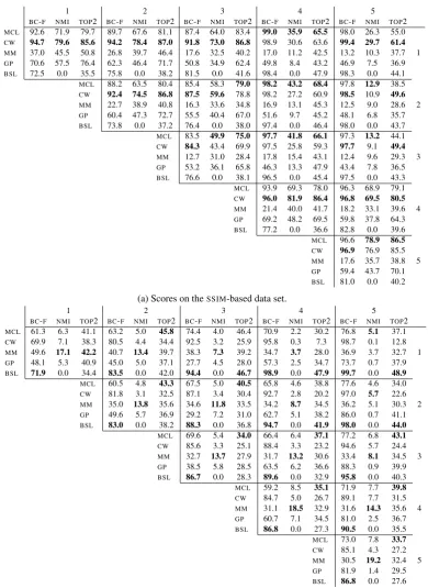
combinations of frequency classes, like the extreme case 1-5, where out of 100 pseudowords this happens 72 times for similarities and 84 times for co-occurrences. On the contrary, when the components belong to the same frequency class, this phenomenon never arises. This can be explained by the fact thatLMI (see Section 2) is proportional to the frequency of a particular context or co-occurrence, so that highly frequent words tend to develop stronger similarities in their distributional thesauri, relegating sparser similarities of less frequent words to a marginal role or outweighing them altogether. Especially in the two highest frequency classes 4 and 5, there are terms that always come to dominate the graphs of their related pseudowords (likebeer).

Interestingly, we notice a drop of theNMIscores for similarities in the fields of Table 2a corre-sponding to the most skewed frequency class com-binations, in particular 1-5, 2-5, 3-5, where some words tend to completely dominate their graphs, and clusterings tend to consist of a single big clus-ter, possibly accompanied by smaller, marginal ones. We also computed a most frequent score baseline (BSL), which yields just one single cluster for each ego word graph. ItsNMIscores are always 0, as this measure heavily penalizes the asymme-try of having just one cluster in the output and two clusters in the ground truth. This, together with the fact that MaxMax, which is the most fine-grained among our examined algorithms, reachesNMI val-ues that are on par with the other systems (or consistently better, in the case of co-occurrences) while regularly obtaining the lowestBC-Fscores, leads us to claim that NMIis biased towards fine-grained clusterings8_{. On the opposite side of the}

spectrum, the more coarse-grained systems tend

8_{This bias is discussed more at length by Li et al. (2014).}

to have very high BC-F scores close to the base-line, especially for the more skewed combinations. This depends on the fact that unbalanced graphs consist of nearly just one sense. Here the bias of BCubed measures becomes manifest: Due to their nature as averages over all single clustered elements, they stress the similarity between the in-ternalstructures of two clusterings, i.e. the distri-bution of elements inside each cluster, and disre-gard theirexternal structures, i.e. their respective sizes and the distribution of cardinalities among clusters. The TOP2 measure, however, was de-fined so as to never assign a score greater than 0.5

in such occurrences. In fact, in the case of co-occurrences we see that the baseline achieves the bestBC-Fscores, but most of the time it is beaten by other systems in terms of TOP2 score. Over-all,TOP2 seems to be the most suited measure for the evaluation of the task represented by our pseu-doword data sets and is more in line with our ex-pectations: higher scores when the ego word graph is more balanced, and much lower scores when the ego word graph is strongly skewed, without the ex-cesses ofNMI.

We remark that scores on the whole are usu-ally worse for co-occurrences than for similarities, both globally and for each frequency class combi-nation. For co-occurrences,TOP2 never goes over 0.5. This is a strong indication that the structure

1 2 3 4 5

BC-F NMI TOP2 BC-F NMI TOP2 BC-F NMI TOP2 BC-F NMI TOP2 BC-F NMI TOP2

MCL 92.6 71.9 79.7 89.7 67.6 81.1 87.4 64.0 83.4 99.0 35.9 65.5 98.0 26.3 55.0

CW 94.7 79.6 85.6 94.2 78.4 87.0 91.8 73.0 86.8 98.9 30.6 63.6 99.4 29.7 61.4

MM 37.0 45.5 50.8 26.8 39.7 46.4 17.6 32.5 40.2 17.0 11.2 42.5 13.2 10.3 37.7 1

GP 70.6 57.5 76.4 62.3 46.4 71.7 50.8 34.9 62.4 49.8 8.4 43.2 46.9 7.5 36.9

BSL 72.5 0.0 35.5 75.8 0.0 38.2 81.5 0.0 41.6 98.4 0.0 47.9 98.3 0.0 44.1 MCL 88.2 63.5 80.4 85.4 58.3 79.0 98.2 43.2 68.4 97.8 12.9 38.5

CW 92.4 74.5 86.8 87.5 59.6 78.8 98.2 27.2 60.9 98.5 10.9 49.6

MM 22.7 38.9 40.8 16.3 33.6 34.8 16.9 13.1 45.3 12.5 9.0 28.6 2

GP 60.4 47.3 72.7 55.5 40.4 67.0 51.6 9.7 45.2 48.1 6.8 35.7 BSL 73.8 0.0 37.2 76.4 0.0 38.0 97.4 0.0 46.4 98.0 0.0 43.7

MCL 83.5 49.9 75.0 97.7 41.8 66.1 97.3 13.2 44.1

CW 84.3 43.4 69.9 97.5 25.8 59.3 97.7 9.1 49.4

MM 12.7 31.0 28.4 17.8 15.4 43.1 12.4 9.6 29.3 3

GP 53.2 36.1 65.8 46.3 13.3 47.9 43.4 7.8 36.5

BSL 76.6 0.0 38.1 96.5 0.0 45.4 97.5 0.0 43.3

MCL 93.9 69.3 78.0 96.3 68.9 79.1

CW 96.0 81.9 86.4 96.8 69.5 80.5

MM 21.4 40.0 41.7 18.2 33.1 39.6 4 GP 69.2 48.2 69.5 59.8 37.8 64.3

BSL 77.2 0.0 36.6 82.8 0.0 39.6

MCL 96.6 78.9 86.5

CW 96.9 76.9 85.5

MM 17.6 35.7 38.8 5

GP 59.4 43.7 70.1

BSL 81.0 0.0 40.2

(a) Scores on theSSIM-based data set.

1 2 3 4 5

BC-F NMI TOP2 BC-F NMI TOP2 BC-F NMI TOP2 BC-F NMI TOP2 BC-F NMI TOP2

MCL 61.3 6.3 41.1 63.2 5.0 45.8 74.4 4.0 46.4 70.9 2.2 30.2 76.8 5.1 37.1

CW 69.9 7.1 38.3 80.5 4.4 34.4 92.5 3.2 25.9 95.8 0.3 7.3 98.7 0.1 12.8

MM 49.6 17.1 42.2 40.7 13.4 39.7 38.3 7.3 39.2 34.7 3.7 28.0 36.9 3.7 32.7 1

GP 48.1 5.3 40.9 45.0 5.0 37.1 27.7 4.5 28.0 57.3 2.5 34.7 73.7 0.7 37.9

BSL 71.9 0.0 34.4 83.5 0.0 42.0 94.4 0.0 46.7 98.9 0.0 47.9 99.7 0.0 48.9

MCL 60.5 4.8 43.3 67.5 5.0 40.5 65.8 4.6 38.8 77.6 4.6 34.0

CW 81.8 3.1 32.5 87.1 3.4 30.4 92.7 2.8 20.2 97.0 5.7 22.6 MM 35.0 13.8 35.6 34.6 11.8 33.5 34.2 8.7 34.5 36.2 5.1 30.3 2

GP 49.6 5.7 36.9 29.2 7.2 31.0 62.7 5.1 38.2 86.0 0.7 41.1

BSL 83.0 0.0 38.2 88.3 0.0 36.8 94.7 0.0 41.9 98.0 0.0 44.0

MCL 69.6 5.4 34.0 66.4 6.4 37.1 77.2 6.8 43.1

CW 85.6 3.3 25.1 88.4 3.3 23.2 94.6 5.7 24.4

MM 32.7 13.7 27.9 31.7 13.2 30.6 33.4 8.1 34.5 3

GP 38.5 5.8 28.5 63.5 6.2 36.6 88.3 0.9 39.9

BSL 86.7 0.0 28.3 89.6 0.0 32.9 95.8 0.0 40.3

MCL 59.2 8.5 35.1 71.9 7.7 39.8

CW 84.7 5.0 26.7 89.1 7.7 31.5

MM 31.1 18.5 32.9 31.6 14.3 35.6 4

GP 60.7 7.1 34.5 81.0 2.5 36.7

BSL 86.8 0.0 27.3 90.5 0.0 35.5 MCL 73.0 7.8 33.7

CW 85.1 4.3 27.2

MM 30.5 19.2 32.4 5

GP 81.9 1.4 29.5

BSL 86.8 0.0 27.6

(b) Scores on the co-occurrence-based data set.

other evaluation measures agree). At the same time, the more fine-grained GP and MCL seem to better adapt to the structure of co-occurrence graphs, while GP’s performances clearly deterio-rate on more unbalanced pseudowords for SSIMs. On the lower end of the spectrum, MaxMax shows a very constant but too divisive nature for our task of homonymy detection.

5.1 Example of Clusterings

We briefly want to show the differences between the clusterings of our four systems (CW, MCL, MaxMax, GP) on the SSIM ego word graph of a same pseudoword. We chose catsup bufflehead: catsup (variant of ketchup) belongs to frequency class 2 and bufflehead (a kind of duck) to fre-quency class 1. Their graph has 488 nodes and a density of 0.548, above the global mean of 0.45. The node ratio is in favour of catsup at 3.05 : 1

against bufflehead, with respectively 111 against 339 exclusive terms, still being a quite balanced ego graph.

Chinese Whispers finds two clusters which seem to cover correctly the two senses of bird or animal on one side, {hummingbird, woodpecker, dove, merganser,..._}, and food on the other side: {polenta, egg, baguette, squab,...}. Its scores are very high, respec-tively 0.95 for BC-F, 0.80 for NMI and 0.93 for

TOP2.

The gangplank algorithm yields 5 clusters. One is clearly about the bird: {goldeneye, condor, peacock,..._}. The other four have high pre-cision, but lose recall for splitting the sense of food, e.g. in {puree, clove, dill,..._} and {jelly, tablespoon, dripping,..._}, and the distinction between them is not always clear. We obtain a BC-F of 0.66, a NMI of 0.51 and a

TOP2 of 0.78.

The Markov cluster algorithm with an inflation factor of 1.4 fails to make a distinction and

finds only one cluster: {raptor, Parmesan, coffee, stork,...}. Its scores are the same of our trivial baseline:BC-F0.77,NMI0.0 andTOP2 0.41 (<0.5, see section 3).

MaxMax confirms its tendency of very fine-grained clusterings and produces 22 clusters. Each has a very high precision, but some consist of only two or three elements, such as {gin, rum, brandy} and {cashmere, denim} and in general they make very narrow distinctions.

The biggest cluster {chili, chily, ginger, shallot,...} has 89 elements. We also find a cluster with bird names, but the overall scores are low:BC-F0.27,NMI0.38 andTOP2 0.45.

6 Conclusions

The major contribution of this work is to present two new pseudoword ego word graph data sets for graph-based homonymy detection: one for context semantic similarities and one for co-occurrences. The data sets are modelled around 1225 pseu-dowords, each representing the combination of two monosemous words. We show that many ego word graphs are too skewed when the two compo-nents come from very different frequency classes, up to the point of actually collapsing on just one sense, but in general they represent a good approx-imation of homonymy. We evidence the biases of BCubed measures and NMI, respectively towards baseline-like clusterings (andBSLis the best per-forming system for co-occurrences in this sense) and finer clusterings. On the contrary, our pro-posed TOP2 metric seems to strike the right bal-ance and to provide the most meaningful scores for interpretation. Chinese Whispers, which yields tendentially coarse clusterings, emerges as the best system overall for this task with regard to SSIM, and is closely followed by MCL, which is in turn the best system for co-occurrences, according to TOP2. The more fine-grained GP approach falls in-between. MaxMax systematically has the low-est scores, as its clusterings prove to be too frag-mented for our task, and only achieves goodNMI values, which are however biased.

These considerations lead us to identify Word Sense Discrimination9 _{(WSD), commonly used as}

a synonym for Word Sense Induction, as an actu-ally different, yet complementary task which ne-cessitates different instruments, as exemplified by our double data set: whereasWSIis paradigmatic, WSDis syntagmatic. We deem that this distinction deserves further investigation. As a future work, beyond expanding our data sets we envision the implementation of consensus clustering (Ghaemi et al., 2009) and re-clustering techniques to im-prove results, and a more accurate analysis of the relation between creation of word graphs and al-gorithms’ outputs.

9_{Defined as “determining for any two occurrences [of a}

References

Enrique Amig´o, Julio Gonzalo, Javier Artiles, and Fe-lisa Verdejo. 2009. A comparison of extrinsic clustering evaluation metrics based on formal con-straints. Information retrieval, 12(4):461–486.

Amit Bagga and Breck Baldwin. 1998. Algorithms for scoring coreference chains. In Proceedings of the first international Conference on Language Resources and Evaluation (LREC’98), workshop on linguistic coreference, pages 563–566, Granada, Spain. European Language Resources Association.

Osman Bas¸kaya and David Jurgens. 2016. Semi-supervised learning with induced word senses for state of the art word sense disambiguation. Journal of Artificial Intelligence Research, 55:1025–1058.

Chris Biemann and Uwe Quasthoff. 2009. Networks generated from natural language text. In Dynam-ics on and of complex networks, pages 167–185. Springer.

Chris Biemann and Martin Riedl. 2013. Text: Now in 2D! a framework for lexical expansion with con-textual similarity. Journal of Language Modelling, 1(1):55–95.

Chris Biemann. 2006. Chinese whispers: an effi-cient graph clustering algorithm and its application to natural language processing problems. In Pro-ceedings of the first workshop on graph based meth-ods for natural language processing, pages 73–80, New York, New York, USA.

Stefan Bordag. 2006. Word sense induction: Triplet-based clustering and automatic evaluation. In Pro-ceedings of the 11th Conference of the European Chapter of the Association for Computational Lin-guistics, pages 137–144, Trento, Italy. EACL.

Flavio Massimiliano Cecchini and Elisabetta Fersini. 2015. Word sense discrimination: A gangplank al-gorithm. InProceedings of the Second Italian Con-ference on Computational Linguistics CLiC-it 2015, pages 77–81, Trento, Italy.

Marie-Catherine De Marneffe, Bill MacCartney, and Christopher Manning. 2006. Generating typed de-pendency parses from phrase structure parses. In

Proceedings of the fifth international Conference on Language Resources and Evaluation (LREC’06), pages 449–454, Genoa, Italy. European Language Resources Association.

Ferdinand De Saussure. 1995 [1916]. Cours de lin-guistique g´en´erale. Payot&Rivage, Paris, France. Critical edition of 1st 1916 edition.

Stefan Evert. 2004. The statistics of word cooccur-rences: word pairs and collocations. Ph.D. thesis, Universit¨at Stuttgart, August.

William Gale, Kenneth Church, and David Yarowsky. 1992. Work on statistical methods for word sense

disambiguation. In Technical Report of 1992 Fall Symposium - Probabilistic Approaches to Natural Language, pages 54–60, Cambridge, Massachusetts, USA. AAAI.

Reza Ghaemi, Md Nasir Sulaiman, Hamidah Ibrahim, Norwati Mustapha, et al. 2009. A survey: clustering ensembles techniques. World Academy of Science, Engineering and Technology, 50:636–645.

Zellig Harris. 1954. Distributional structure. Word, 10(2-3):146–162.

Taher Haveliwala. 2002. Topic-sensitive pagerank. In

Proceedings of the 11th international conference on World Wide Web, pages 517–526, Honolulu, Hawaii, USA. ACM.

David Hope and Bill Keller. 2013. MaxMax: a graph-based soft clustering algorithm applied to word sense induction. InProceedings of the 14th Interna-tional Conference on ComputaInterna-tional Linguistics and Intelligent Text Processing, pages 368–381, Samos, Greece.

David Jurgens and Ioannis Klapaftis. 2013. SemEval-2013 task 13: Word sense induction for graded and non-graded senses. In *SEM 2013: The Second Joint Conference on Lexical and Computational Se-mantics, volume 2, pages 290–299, Atlanta, Geor-gia, USA. ACL.

Adam Kilgarriff, Pavel Rychl´y, Pavel Smrˇz, and David Tugwell. 2004. The sketch engine. InProceedings of the Eleventh Euralex Conference, pages 105–116, Lorient, France.

Linlin Li, Ivan Titov, and Caroline Sporleder. 2014. Improved estimation of entropy for evaluation of word sense induction. Computational Linguistics, 40(3):671–685.

Suresh Manandhar, Ioannis Klapaftis, Dmitriy Dligach, and Sameer Pradhan. 2010. Semeval-2010 task 14: Word sense induction & disambiguation. In Pro-ceedings of the 5th international workshop on se-mantic evaluation, pages 63–68, Los Angeles, Cal-ifornia, USA. Association for Computational Lin-guistics.

James Martin and Daniel Jurafsky. 2000. Speech and language processing. Pearson, Upper Saddle River, New Jersey, USA.

George Miller. 1995. WordNet: a lexical database for English. Communications of the ACM, 38(11):39– 41.

Roberto Navigli, Kenneth Litkowski, and Orin Har-graves. 2007. SemEval-2007 task 07: Coarse-grained English all-words task. In Proceedings of the 4th International Workshop on Semantic Evalu-ations, pages 30–35, Prague, Czech Republic. Asso-ciation for Computational Linguistics.

Roberto Navigli. 2009. Word sense disambiguation: A survey. ACM Computing Surveys (CSUR), 41(2):10.

Lubom´ır Otrusina and Pavel Smrˇz. 2010. A new ap-proach to pseudoword generation. InProceedings of the seventh international Conference on Language Resources and Evaluation (LREC’10), pages 1195– 1199. European Language Resources Association.

Robert Parker, David Graff, Junbo Kong, Ke Chen, and Kazuaki Maeda. 2011. English Gigaword Fifth Edition. Linguistic Data Consortium, Philadelphia, Pennsylvania, USA.

Mohammad Taher Pilehvar and Roberto Navigli. 2013. Paving the way to a large-scale pseudosense-annotated dataset. InProceedings of the 2013 Con-ference of the North American Chapter of the Asso-ciation for Computational Linguistics: Human Lan-guage Technologies (HTL-NAACL), pages 1100– 1109, Atlanta, Georgia, USA. Association for Com-putational Linguistics.

Steffen Remus and Chris Biemann. 2013. Three knowledge-free methods for automatic lexical chain extraction. In Proceedings of the 2013 Confer-ence of the North American Chapter of the Associ-ation for ComputAssoci-ational Linguistics: Human Lan-guage Technologies (HTL-NAACL), pages 989–999, Atlanta, Georgia, USA. Association for Computa-tional Linguistics.

Matthias Richter, Uwe Quasthoff, Erla Hallsteinsd´ottir, and Chris Biemann. 2006. Exploiting the Leipzig Corpora Collection. In Proceedings of the Fifth Slovenian and First International Language Tech-nologies Conference, IS-LTC ’06, pages 68–73, Ljubljana, Slovenia. Slovenian Language Technolo-gies Society.

Keijo Ruohonen. 2013. Graph Theory. Tampereen teknillinen yliopisto. Originally titled Graafiteoria, lecture notes translated by Tamminen, J., Lee, K.-C. and Pich´e, R.

Hinrich Sch¨utze. 1992. Dimensions of meaning. In

Proceedings of Supercomputing’92, pages 787–796, Minneapolis, Minnesota, USA. ACM/IEEE.

Hinrich Sch¨utze. 1998. Automatic word sense dis-crimination. Computational linguistics, 24(1):97– 123.

Alexander Strehl. 2002. Relationship-based cluster-ing and cluster ensembles for high-dimensional data mining. Ph.D. thesis, The University of Texas at Austin, May.

Peter Turney and Patrick Pantel. 2010. From fre-quency to meaning: Vector space models of se-mantics. Journal of artificial intelligence research, 37(1):141–188.

Stijn van Dongen. 2000.Graph clustering by flow sim-ulation. Ph.D. thesis, Universiteit Utrecht, May.