The effect of protein dielectric coefficient on the ionic selectivity of a calcium channel

The effect of protein dielectric coefficient on the ionic selectivity

of a calcium channel

DezsőBodaa兲

Department of Molecular Biophysics and Physiology, Rush University Medical Center, Chicago, Illinois 60612 and Department of Physical Chemistry, Pannon University, P.O. Box 158, H-8201, Veszprém, Hungary

Mónika Valiskó

Department of Physical Chemistry, Pannon University, P.O. Box 158, H-8201, Veszprém, Hungary

Bob Eisenberg

Department of Molecular Biophysics and Physiology, Rush University Medical Center, Chicago, Illinois 60612

Wolfgang Nonner

Department of Physiology and Biophysics, University of Miami School of Medicine, Miami, Florida 33101

Douglas Henderson

Department of Chemistry and Biochemistry, Brigham Young University, Provo, Utah 84602

Dirk Gillespie

Department of Molecular Biophysics and Physiology, Rush University Medical Center, Chicago, Illinois 60612

共Received 21 April 2006; accepted 17 May 2006; published online 18 July 2006兲

Calcium-selective ion channels are known to have carboxylate-rich selectivity filters, a common motif that is primarily responsible for their high Ca2+_{affinity. Different Ca}2+_{affinities ranging from}

micromolar 共the L-type Ca channel兲 to millimolar 共the ryanodine receptor channel兲 are closely related to the different physiological functions of these channels. To understand the physical mechanism for this range of affinities given similar amino acids in their selectivity filters, we use grand canonical Monte Carlo simulations to assess the binding of monovalent and divalent ions in the selectivity filter of a model Ca channel. We use a reduced model where the electolyte is modeled by hard-sphere ions embedded in a continuum dielectric solvent, while the interior of protein surrounding the channel is allowed to have a dielectric coefficient different from that of the electrolyte. The induced charges that appear on the protein/lumen interface are calculated by the induced charge computation method关Bodaet al., Phys. Rev. E 69, 046702共2004兲兴. It is shown that decreasing the dielectric coefficient of the protein attracts more cations into the pore because the protein’s carboxyl groups induce negative charges on the dielectric boundary. As the density of the hard-sphere ions increases in the filter, Ca2+ is absorbed into the filter with higher probability than Na+ because Ca2+ provides twice the charge to neutralize the negative charge of the pore 共both structural carboxylate oxygens and induced charges兲 than Na+ while occupying about the same space共the charge/space competition mechanism兲. As a result, Ca2+affinity is improved an order of magnitude by decreasing the protein dielectric coefficient from 80 to 5. Our results indicate that adjusting the dielectric properties of the protein surrounding the permeation pathway is a possible way for evolution to regulate the Ca2+ affinity of the common four-carboxylate motif. © 2006 American Institute of Physics.关DOI:10.1063/1.2212423兴

I. INTRODUCTION

Calcium ions control many biological functions by acti-vating molecular switches in the cytoplasm. Therefore, cyto-solic Ca2+ _{concentrations are actively maintained at}

submi-cromolar levels, and the molecular switches are activated when Ca2+_{enters the cytoplasm from storage sites inside the}

cell or from the extracellular space. Both of these

intracellu-lar and extracelluintracellu-lar compartments contain 1 – 3 mM concen-trations of free Ca2+_{共i.e., Ca}2+_{not bound to proteins such as}

calsequestrin兲and both are separated from the cytoplasm by a lipid membrane. Ca2+ _{crosses these particular membranes}

through molecular pores formed by channel proteins. When these ion channels open, they selectively conduct Ca2+ _and

therefore refered to as calcium共Ca兲channels. Selectivity for Ca2+_{is vital for their biological function because most of the}

ions nearby are not Ca2+_{. The most abundant other ions are}

Na+_{共in the extracellular space兲and K}+_{共inside the cell and its}

compartments兲, typically both at concentrations of

approxi-a兲_{Author to whom correspondence should be addressed. Electronic mail:}

dezsoគ[email protected]

mately 150 mM. To conduct Ca2+_{, Ca channels must}

over-come a 100:1 unfavorable concentration ratio of monovalent ions to Ca2+_.

Different Ca channels conduct different amounts of Ca2+

under identical conditions. For example, in single-channel recordings of current/voltage curves with 100 mM Na+or K+ on both sides of the membrane, a few micromolars of added Ca2+ _{is enough to reduce the monovalent current by half}

共compared to the current in 0 Ca2+_{兲in theL-type Ca channel.}

On the other hand, it takes 1000 times as much Ca2+_{共a few}

millimolars兲to have the same effect in the ryanodine recep-tor共RyR兲Ca channel.1Although it is not practical to experi-mentally measure the different ionic compositions of the L-type or RyR currents, the measureable change in the net current as bath Ca2+ concentration increases from zero indi-cates that Ca2+ current increases as well. This change in the ionic components of current must reflect changing channel occupancies of Ca2+ _{and, for example, Na}+_{. Here we use}

equilibrium Monte Carlo共MC兲simulations to study channel occupancy 共as bath Ca2+ _{concentration increases兲 to assess}

the “affinity” of our model channel for Ca2+_.

The different selectivities of theL-type Ca channel and RyR for Ca2+ are important for the different physiological functions of these channels. For example, the L-type Ca channel of cardiac and skeletal muscle controls Ca2+ move-ment from the extracellular compartmove-ment. The action of the L-type channel opens RyR that controls the release of Ca2+

from intracellular stores. This large release of Ca2+_over

sev-eral milliseconds initiates muscle contraction. The enormous selectivity ofL-type Ca channels allows Ca2+_{to dominate in}

the pore and thereby preclude—in effect “block”—the flux of monovalent ions such as Na+through theL-type channel under physiological conditions.2On the other hand, a model of ion permeation through RyR共Ref. 3兲 has shown that the weaker selectivity of RyR allows conduction of both Ca2+

and K+_{under the same conditions. Conduction of Ca}2+_{out of}

the intracellular stores with simultaneous conduction of K+

in the opposite direction may be one way for RyR to keep the electrostatic potential across the channel near zero and thus sustain Ca2+ _{release over several milliseconds.}4

Mutation studies on both theL-type Ca channel and RyR have identified the amino acids primarily responsible for the Ca2+_{selectivity of these channels. In theL-type Ca channel,}

four glutamates 共the EEEE locus兲 were found essential for selectivity,5–7 while in RyR, four aspartates were identified that give RyR a DDDD locus.8 共In RyR, two other amino acids—one glutamate and one aspartate—also affect Ca2+

selectivity, but to a lesser extent.9,10兲These glutamates and aspartates are similar amino acids with a carboxylate group 共COO−_{兲 at the end of the side chain. Therefore, both the}

L-type Ca channel and RyR have carboxylate-rich selectivity filters, but very different Ca2+ _{versus monovalent}

selectivi-ties. This paper addresses how similar selectivity filters can produce significantly different Ca2+ _{affinities by examining}

how the polarization properties of the protein affect Ca2+

affinity.

Carboxylate-rich loci have also been observed in pro-teins other than ion channels. Many Ca2+-selective proteins have Ca2+ binding sites in cavities lined by oxygen atoms11

from carboxylate groups of amino acids. In addition to car-boxylate groups, in the EF-hand motif observed in many Ca2+ binding proteins,12 oxygens of hydroxyl or carbonyl groups and a water molecule are also involved in coordinat-ing Ca2+_{. Like Ca channels, proteins with EF-hand motifs}

共for which crystallographic information exists13兲have differ-ent Ca2+ affinities.12

The nature of the high Ca2+ _{affinity of the L-type Ca}

channel is a matter of debate.14–24 In order to quantify the various energy terms, Nonner and Eisenberg used an ex-tended Poisson-Nernst-Planck 共PNP兲 description of L-type Ca channels to estimate the excess chemical potentials needed to produce the experimentally observed specificities.22Subsequent calculations using only bulk elec-trolyte theories18,21 showed that the excess chemical poten-tials needed to produce selectivity could arise from simple physical effects. Correlations produced by the finite diameter of the ions accounted for most of the excess free energy producing selectivity; no other chemical forces were neces-sary. We have also shown that such calculations with bulk solutions are qualitatively共and often quantitatively兲accurate when compared to results computed in confining channel geometries.25The reduced model of the Ca channel that was developed from this theoretical work was reexamined using MC simulations, similar to the simulations in this paper.16,17,20

The results of all these works led to the hypothesis that Ca channel selectivity is produced, to first order, by a com-petition of charged ions for room in a crowded space 关the charge/space competition 共CSC兲 mechanism兴. In recent years, CSC has been successfully tested in several experi-mental situations:共1兲by engineering Ca2+_{-selective channels}

through modification of the OmpF porin;26,27 共2兲by confer-ring Ca2+sensitivity to pores in abiotic plastic membranes;28 and 共3兲 by reproducing—and predicting—a wide range of experimental data from RyR with alkali metal and alkali earth cations3using a CSC-based theory that combined PNP and density functional theory 共DFT兲of fluids.29,30 The suc-cess of this RyR modeling supports both the CSC mechanism and the idea that the movement of finite size ions through the pore can be described by the basic equations of electrodiffu-sion共PNP兲without additional specific chemical forces.

Here we continue our study of model Ca channels with equilibrium calculations of channel occupancy. To make the complex link between occupancy and experimentally mea-sureable currents requires a theory of ion permeation, for example, PNP/DFT 共Refs. 29 and 30兲 or Brownian dynamics.14,15,19,23,24 However, studying only ion accumula-tion in a channel at equilibrium reduces the complexity of the problem and allows us to use the grand canonical 共GC兲 ensemble to simulate micromolar Ca2+concentrations.

In our study, we determine the binding affinity of our model Ca channel as the dielectric properties of the protein are changed. We show that changes in the dielectric environ-ment can shift Ca2+_{affinities from the millimolar range into}

tool that allows evolution to regulate the Ca2+ _{specificity of}

the common carboxylate motif, although we do not believe it to be the only such tool.

Dielectric properties of channel walls have previously been considered,31–35 most recently by Chung et al. in Brownian dynamics studies of ion conduction through Ca channels.14,15,19,23,24 The lowest bath concentration of Ca2+

tested in their simulations was 18 mM共corresponding to one Ca2+_{in the system兲. Affinity in the micromolar range of bath}

Ca2+_{concentration was estimated by an extrapolation over a}

range of 104_{, from 18 to 0.001 mM based on kinetics. Here,}

affinity in the micromolar range was simulated directly with bath Ca2+ concentrations from 10 to 0.012 mM—without extrapolation—using the GC ensemble.

The dielectric inhomogeneity that appears at the bound-ary of the electrolyte solution and the protein raises substan-tial numerical difficulties regarding both the accuracy and efficiency of the method used to calculate the electrostatics. With regard to accuracy, the dependence of results on the resolution of the numerical calculations and problems due to curved dielectric boundaries had to be checked, while with regard to efficiency, the electrostatic energy had to be up-dated in every simulation step. We deal with these difficulties by using the induced charge computation 共ICC兲 method.36 We discuss the method and show its accuracy in the channel geometry considered in this work.

II. MODEL

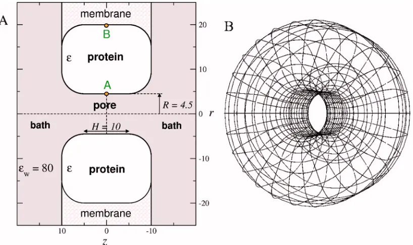
We simulate a Ca channel containing the four-carboxylate motif and ions of an electrolyte bath in a reduced model. Figure1共a兲shows a central cross section of the simu-lation cell; the three-dimensional共3D兲geometry is obtained by rotating one-half of Fig.1共a兲around the axis defined by

r= 0关Fig.1共b兲兴. There is also symmetry with respect to the plane z= 0 that allows us to average results obtained in cor-responding positions of both half-cells. The protein forming the wall of the aqueous pore and the cell membrane sur-rounding the protein are represented as a region that is bounded by hard walls. The protein surface forms a sharp dielectric boundary that encloses a region of共varied兲 dielec-tric coefficient⑀and separates it from the uniform dielectric in the rest of the cell共assigned the dielectric coefficient 80, a value characteristic of aqueous solutions兲. We use a dielectric coefficient of 80共rather than 2兲for the membrane region to reduce the computational effort for the electrostatics; con-trols showed no significant effect on the results of interest 共see Fig. 1 of the supplementary material37兲.

The four carboxylate groups of the protein channel are modeled as eight half-charged anions with a radius of 1.4 Å that are restricted to the cylindrical part of the pore 共radius R= 4.5 Å and length H= 10 Å兲 but are free to move within this region. These “oxygen ions” are confined within the cy-lindrical pore region共兩z兩艋3.6 Å兲where they are not allowed to overlap with the wall of the pore 共r艋3.1 Å兲.

Ions共Na+_{, Ca}2+_{, and Cl}−_{兲are modeled as charged hard}

spheres共rNa= 1 Å,rCa= 0.99 Å, andrCl= 1.81 Å兲and are

al-lowed to distribute within the “solution” region, which in-cludes the pore and the two baths. The solvent is represented as a uniform dielectric with a dielectric coefficient of 80. Ions are confined to the simulation cell by hard walls, but CaCl₂ salt can be exchanged against a large reservoir of a chosen chemical potential, as detailed below. The dimen-sions of the bath regions are large enough to allow the for-mation of bulklike electrolytes in the centers of the baths.

The aqueous dielectric extends into the space outside the cell. The simulation includes a single, rather than periodi-cally replicated, simulation cell.

III. METHODS

A. Monte Carlo simulations

We use the standard Metropolis algorithm38–40 in a mixed ensemble. The volume of the simulation cellVand the temperature T= 298 K are constant, the number of Na+ is fixed, and the numbers of Ca2+and Cl−are allowed to fluc-tuate as in a grand canonical ensemble. Three kinds of MC steps are used.

共1兲Simple particle displacement. We attempt to displace a randomly chosen ion to a randomly chosen position in two ways:共a兲within a fixed neighborhood of its original position 共useful in sampling high-density regions like the pore兲or共b兲 anywhere in the simulation cell 共useful in sampling low-density regions like the bath兲. In both cases, the acceptance probability is p= min关1 , exp共−⌬U/kT兲兴, where k is the Boltzmann constant and⌬Uis the energy change of the sys-tem in the MC step.

共2兲Biased particle displacement between pore and bath. When only simple displacements are allowed, ions rarely move between the pore and the baths because共1兲 a particle rarely attempts toleavethe pore because the number of par-ticles in the pore is small, and共2兲a particle rarely attempts to enter the pore because the volume of the pore is small. To improve sampling and accelerate convergence of the average number of different ions in the pore, we move a randomly chosen ion located in the pore to the bath, or vice versa. The bias inherent to this kind of displacement is accounted for by the acceptance probability

pbias= min

冋

exp

冉

kT

冊

册

where Vnew and Vold are the volumes of the two

compart-ments between which the ion is moved.16

共3兲Particle insertion/deletion. Because we wish to study Ca2+_{absorption from a very dilute Ca}2+_{bath, we equilibrate}

CaCl2 between the simulation cell and a reservoir of given

chemical potential. Following the grand canonical method of Ref. 41, we insert 1 Ca2+ _{and 2 Cl}− _{at random positions in}

the simulation cell or we delete 1 Ca2+ _{and 2 Cl}− _{that are}

randomly chosen from the simulation cell, subject to the ac-ceptance probability

pGC= min

冋

冉

冊

␯

exp

冉

冊

册

共2兲

with

B=␮Ca+ 2␮Cl+ lnVCa ␭Ca

3 + 2 ln

V_Cl

␭Cl

3 , 共3兲

and

␭i=

h 共2␲mikT兲1/2

. 共4兲

N_CaandN_Clare the numbers of the ions in the cell before the operation,␮iis the chemical potential, andmiis the mass of

the ionic speciesi.VCaandVCl are the volumes of the cell

region accessible to the respective ionic species. The value of

␯is 1 for insertion and −1 for deletion. Choosing a value for B uniquely defines the grand canonical step and the average bath Ca2+_{concentration.}

Both insertion and deletion of CaCl2 are attempted in

25% of the trials. In the other half of the trials, an ionic species is chosen at random and simple or biased displace-ments are attempted with equal weights. Trials are parti-tioned this way to speed up convergence; the partitioning does not affect the final result of the MC simulation.38–40 Only simple displacements are attempted for the structural oxygen ions that are confined within the pore cylinder.

The purpose of the simulations was to determine the pore’s absorption of ions from a bath with 0.1M NaCl and a variable amount of added CaCl2for different dielectric

coef-ficients⑀of the protein共2, 5, 10, 20, 40, and 80兲. Appropri-ate cell dimensions were determined in preliminary simula-tions. A cell containing 300 Na+_{in a cylinder 75 Å in radius}

and 320 Å in length gave nearly identical results as cells containing 200 or 400 Na+_{in appropriate volumes共Fig. 3 of}

the supplementary material37兲; therefore, the cell with 300 Na+_{was used in production runs. The concentration of Ca}2+

in the baths was varied between 12␮M and 10 mM by vary-ing the value of the parameterBin Eq.共2兲. In the absence of Ca2+_{, canonical simulations were done to determine the}

ab-sorption of Na+_{from the pure 0.1M NaCl bath. The}

statisti-cal errors indicated in graphs are the standard deviations of 20–99 runs starting from different seeds. Each run included 6⫻108_{– 9⫻10}8_{MC trials.}

B. Electrostatics

The simulations involve the electrostatic energy of a sys-tem whose source charge with density ␳共r兲 is embedded in nonuniform polarizable matter. The electrical fieldE includ-ing the polarizationP is described by Poisson’s equation,

⑀0ⵜ ·E共r兲=␳共r兲−ⵜ·P共r兲. 共5兲

In our reduced model of the Ca channel, we describe the polarization by the linear constitutive relation

P共r兲=共⑀共r兲− 1兲⑀0E共r兲, 共6兲

where ⑀共r兲 is the location-dependent dielectric coefficient. Using Eqs. 共5兲 and共6兲, the polarization charge densityh共r兲 = −ⵜ·P共r兲can be expressed as

h共r兲=1 −⑀共r兲

⑀共r兲 ␳共r兲−⑀0 ⵜ⑀共r兲

⑀共r兲 ·E共r兲. 共7兲

element by the electric field where the dielectric is spatially nonuniform.

In our simulations, the source charge is a set of point charges 共located at the center of hard-sphere ions兲 so ␳共r兲 =兺kqk␦共r−rk兲, whereqkis the charge of thekth point charge

located atrk. Furthermore, the dielectrics in our simulations

form regions of constant dielectric coefficient separated by a sharp boundary surfaceB. Hence, charge is only induced on the infinitesimal surface of each共point兲source charge共h共rk兲兲

and on the boundary surfaceB共h共s兲兲,

h共r兲=␦共r−rk兲h共rk兲+␦共r−s兲h共s兲

=␦共r−rk兲

兺

1 −⑀共rk兲

⑀共rk兲

qk−␦共r−s兲⑀0

⌬⑀共s兲

⑀

¯共s兲 n共s兲·E共s兲, 共8兲

wheresis any location onB,⌬⑀共s兲is the change of dielec-tric coefficient in the normal direction n共s兲of the dielectric boundary, and¯⑀共s兲is the mean of the dielectric coefficients at the boundary location. By Coulomb’s law and superposi-tion, the electric field at the boundary is

E共s兲= 1 4␲⑀0

冕

s−s

⬘

兩s−s

⬘

⬘

⬘

+ 1 4␲⑀0

兺

qk

⑀共rk兲

s−rk

兩s−rk兩3

. 共9兲

Inserting Eq.共9兲into Eq.共8兲yields the integral equation for h共s兲,

h共s兲+ ⌬⑀共s兲

4␲⑀¯共s兲n共s兲·

冕

⬘

兩s−s

⬘

⬘

⬘

= − ⌬⑀共s兲

4␲⑀¯共s兲n共s兲·

兺

qk

⑀共rk兲

s−rk

兩s−rk兩3

. 共10兲

When the integral equation in h共s兲 is solved on the two-dimensional boundary B, all source and induced charges of the system are known and the electrical field at any location can be computed using Coulomb’s law and superposition. This method of determining the electrical field is computa-tionally more efficient than solving Poisson’s equation in three dimensions.

This ICC method has been derived previously36,42 from the variational approach of Allenet al.43–46Integral equation methods have been used, e.g., in work computing apparent surface charges 共ASC兲 in polarizable continuum models 共PCM兲 of solvation of macromolecules.47–52 Reducing the surface integral equation to a system of linear equations yields the boundary element method53–57共BEM兲also used by Green and Lu58,59and Lu and Green60in their simulations of ion channels.

In our simulations, ions共source charges兲move within a uniform region of dielectric共the pore lumen and bath兲but do not move between regions with different dielectrics. The part of the electrostatic energy that varies due to such a relocation of a source charge is

UES= 1 2

兺

k

qk

4␲⑀0

冉

兺

qj

⑀共rj兲兩rk−rj兩

+

冕

h共s兲 兩s−rk兩

ds

冊

共11兲

1. Discretization of the dielectric boundary

The simulation of the ion channel system involves di-electric boundaries that are curved共Fig.1兲. In evaluating the surface integral of Eq. 共10兲, the surface curvature and the spatial variation of the surface charge create numerical diffi-culties, and the resulting algorithms and codes have to be checked carefully for accuracy and efficiency in our experi-ence. We discretize the dielectric boundary surface as a set of two-dimensional boundary elements called “tiles”B_␣of gen-erally nonuniform size. The charge induced on each tileh_␣is approximated as uniform over the tile and is computed from the field strength acting in the normal directionn_␣=n共s_␣兲at the center of charges_␣ of the tile’s areaa_␣.

Discretizing Eq.共10兲this way yields the system of linear equations

兺

冋

4␲⑀¯_␣I␣␤

册

⌬⑀␣ 4␲⑀¯_␣

兺

qk

⑀共rk兲

共s␣−rk兲

兩s␣−rk兩3

·n_␣,

共12兲

with

I_␣␤=

冕

共s_␣−s

⬘

兩s_␣−s

⬘

⬘

where⌬⑀_␣=⌬⑀共s_␣兲,¯⑀_␣=¯⑀共s_␣兲, and␦_␣␤is the Kronecker delta function. These equations can be written in matrix notation as

Ah=c, 共14兲

where each element of the matrixAis given by the expres-sion in square brackets in Eq.共12兲, each element of the col-umn vectorhis given byh_␤, and each element of the column vector c is given by the right-hand side of Eq.共12兲. For a given configuration of source charges, the right-hand side of Eq. 共12兲is known. Hence, the system can be solved for the induced charge densities h. Since the matrix Ais dense, we use LU decomposition. This decomposition becomes part of the simulation overhead because A does not change when source charges are moved in the cell. The system can be solved for varied positions 共and numbers兲 of the source charges by backsubstitution.

The discretized formula for the electrostatic energy is

UES= 1 2

兺

k

qk

4␲⑀0

冉

兺

qj

⑀共rj兲兩rk−rj兩

+

兺

h_␤J_␤

冊

with

J_␤=

冕

ds 兩s−rk兩

2. Choosing discretization parameters

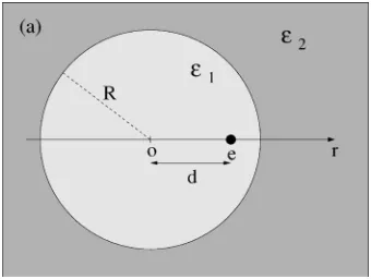
The accuracy of the boundary discretization depends on both the choice of tile size and on the method of evaluation of the integralsI_␣␤andJ_␤. The tile size needs to be chosen small enough so that the electric field 共and hence induced charge density兲are sufficiently uniform within the area of the tile. The integration method is particularly important when the surface is curved. Then, charge induced on the same tile contributes to the normal electric field in the center of the tile, and these contributions are large because of the short distances. Nearby charge can induce charge on a tile as well. We have determined the tile size and evaluated different ap-proximations to the integrals using the example of a point charge eccentrically located inside a dielectric sphere 共Fig. 2兲. This example involves surface curvature and inhomoge-neity of induced charge. Both are important. An analytical solution in terms of Legendre polynomials is known.61 We consider a sphere radius共5 Å兲and dielectric coefficients共80 and 2兲 that are relevant for our simulations. Figure 3 plots

analytical and numerically computed potentials for a case in which the source charge is located 1 Å from the boundary. The potential is that generated by the charge induced on the sphere, along the straight line connecting source charge and sphere center 共Fig. 2兲. The interaction of the source charge with its own induced charge is given by the potential at the positionr= 4 Å.

In a first approximation to the integralsI_␣␤ andJ_␤, the surface charge of the tile is represented as a point charge of magnitudeh_␣a_␣located at the center of the tile area. Further-more, tiles are assumed to be flat so thatI_␣␣= 0. We call this the point charge 共PC兲 approximation. In a second approxi-mation, the tile is divided inton⫻nsubtiles关n= 10 was used to computeI_␣␤共␣⫽␤兲andn= 20 was used to computeI_␣␣兴. These follow the curvature of the tile and are assigned the same uniform induced charge density of the larger tile. The method of subtiling is detailed for the generalized cylinder geometry in the supplementary material.37 In this method, I_␣␣⫽0 contributes a substantial term due to surface curva-ture. We call the second method the surface charge 共SC兲 approximation.

The potential curves plotted in Fig.3 were obtained us-ing these methods in different combinations. The label SC/ PC/PC indicates that the SC method was used in evaluating I_␣␣, and the PC method in both I_␣␤ 共␤⫽␣兲 and J_␤. The potential computed with PC/PC/PC strongly deviates from the analytical result even though the spherical boundary was discretized into a particularly large number of tiles 共2048兲. The SC/SC/SC method yields far more accurate results with a discretization of 512 tiles; it is more accurate than PC/ PC/PC even when the number of tiles is reduced from 2048 tiles to 128. SC/SC/SC with 2048 tiles is indistinguishable from the analytic curve. SC/SC/PC yields accurate potentials up to positions less than 1 Å away from the dielectric bound-ary. Since ions are excluded from this region in our simula-tions, we use the SC/SC/PC method in production runs. Us-ing the PC method in the computations of energy avoids additional computational cost in evaluatingJ_␤ whenever an ion is moved in the simulation.

Finally, we note that SC/PC/PC produces a larger error than SC/SC/PC. Hence, using the SC method is essential in evaluating I_␣␣, but using the SC method in evaluating I_␣␤ 共␤⫽␣兲still gives a substantial reduction of error compared to the PC method. Correction for boundary curvature have been devised in many implementations of the BEM to con-sider the effects of charge induced on the same surface ele-ment I_␣␣ 共Refs. 23, 47, 49, 53, and 62兲 共see also the reviews63,64兲. Our approximation is based on direct numeri-cal integration rather than analytinumeri-cal corrections based on approximations. We find it necessary to apply the numerical integration also to compute charges induced by the field of other surface elements.

3. Tests of numerical accuracy

No analytical solution is known for the electrostatics of the system that we simulate 共Fig.1兲. Nevertheless, an inde-pendent test of accuracy is possible using Gauss’s law. The dielectric domain of the protein in our simulations contains no source charges. By Gauss’s law, the total charge induced

FIG. 2. Geometry used for assessing boundary discretizations. A spherical dielectric domain 共R= 5 Å, ⑀1= 80兲is embedded in a space containing a different dielectric共⑀₂= 2兲. An elementary point charge is placed inside the sphere at a distanced= 4 Å from the center.

by ions on the closed surface of the protein must equal zero. Figure4 plots computed total surface charges of the protein as a function of the inverse number of tiles used in the dis-cretization of the boundary. The charge on the boundary was induced by a single source charge共1e兲placed at five differ-ent test locations, as shown by the inset of Fig.4.

In a second kind of test, MC runs with the actual simu-lation cell 共Fig. 1兲 were done using discretizations of 540, 690, and 1462 tiles 共Fig. 2 of supplementary material37兲. Concentration profiles were virtually indistinguishable for all choices. Production runs were with the discretization of 690 tiles. The dimension of these tiles was chosen smallest for the wall of the pore共⬇1 Å兲and gradually increased to⬇5 Å in the periphery of the protein关see Fig.1共b兲兴. This choice of discretization explains why the errors in the total induced charge seen in Fig. 4 have little effect on the simulation results 共see Fig. 2 of supplementary material37兲. Errors are mainly due to the coarser discretization of boundary regions far from the pore, which has small effects on the ions in the space of interest, that is, in and near the pore.

IV. RESULTS AND DISCUSSION

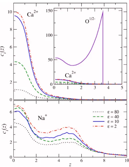
The main results of the simulations are the ionic concen-tration profiles. We first consider whether variation of the protein’s dielectric has qualitative effects on the packing of ions and structural charges in the pore. The longitudinal, cross sectionally averaged profiles of Ca2+_{, Na}+_{, and oxygen}

ion concentrations for different dielectric coefficients are plotted in Fig.5. The structural charges do not rearrange over the range 2艋⑀艋80 and the mobile ions also distribute in a stable pattern as⑀is varied. The dielectric coefficient, how-ever, controls the absolute concentrations of the mobile ions. Although both Ca2+ and Na+ are strongly absorbed into the pore, Ca2+ is absorbed over Na+as the dielectric coefficient

is reduced. Unlike Ca2+, Na+ absorption increases more strongly near the pore mouths than at the pore center.

The radial distributions of the mobile and structural ions also only undergo gradual quantitative variations as the di-electric coefficient is varied. Figure 6 shows concentration profiles in both the axial and radial dimensions of the pore for⑀= 10. The oxygen ions dwell near the pore walls, except at the ends of the pore, where they spread more evenly over the cross section. The central space of the pore is occupied by Ca2+ and Na+that are screened in this way by a shell of oxygen ions. Ca2+ always packs near the pore axis, whereas Na+ _{is more spread out over the cross section. The same}

pattern is seen when⑀= 80共not shown兲. Overall, the packing of the particles in the pore is not qualitatively changed by varying the protein dielectric. It appears that the presence of the dielectric boundary more or less enhances a pattern of packing that is already stable due to screening and excluded-volume interactions among the charged particles in the pore. To present our simulation results for different⑀in a con-cise way, we distill the concentration profiles into a single number, the occupancy of an ionic species. For each ionic species, the affinity of the channel for that species is charac-terized by its occupancy, while the selectivity is character-ized by the relative occupancies of the two ionic species. For this we have to define the region of the pore兩z兩艋⌬H/ 2 over which we integrate the ionic profiles to calculate the average number of each ionic species. Figure5 shows that Ca2+ ac-cumulates in the center of the pore, while Na+accumulates both in the center of the pore and in the atria. Therefore the choice of ⌬H will affect the calculated occupancy. One

FIG. 4. 共Color online兲Sum rule test based on Gauss’s law. An elementary point charge is placed at various locations共see inset兲in or near the pore of the simulation cell关compare Fig.1共a兲兴. Points 1, 3, and 5 are on the center-line, while points 2 and 4 are 1 Å from the pore wall. Points 1 and 2 are in the middle in the pore, while points 3 and 4 are at the entrance of the pore. Point 5 is in the solution near the pore. The charge induced on the protein surface has been integrated and plotted vs the inverse number of tiles used in the surface discretization. The exact result from Gauss’s law is that the charge induced on the protein is zero because the protein region does not enclose any source charges共Ref.61兲.

FIG. 5.共Color online兲Longitudinal packing of mobile and structural ions in the pore. The concentration profiles are averaged over the cross section. The bath contains 8.6⫻10−5_MCaCl

choice is the whole length of the cylindrical pore 共⌬H = 10 Å兲. We also consider the central region of the pore 共⌬H= 4.2 Å兲, where Ca2+ _{accumulates more favorably than}

Na+_{as⑀is decreased. Figure7shows the average number of}

Ca2+_{and Na}+_{accumulated in the whole pore cylinder共10 Å}

long兲 and in the central pore region 共4.2 Å long兲 for two fixed CaCl2 concentrations as functions of the dielectric

co-efficient of the protein. The accumulations in the two regions are similar for Ca2+_{, which is concentrated in the central}

region. The accumulations of Na+ _{differ more substantially}

between the two regions because Na+_{also accumulates in the}

pore region outside the central region.

The competitive accumulation of counterions in the charged pore defines the selectivity of the system, a measure of immediate biological interest. Figure 8 shows, for each protein dielectric coefficient that was tested, the number of

Ca2+ _{and Na}+ _{accumulated in the pore cylinder 共⌬H}

= 10 Å兲from baths containing 0.1M NaCl and a varied con-centration of CaCl₂ 共curves calculated with ⌬H= 4.2 Å are seen in Fig. 4 of the supplementary material37兲. Reducing the dielectric coefficient of the protein enhances the accumula-tions of both ions, Ca2+and Na+. The bath CaCl2

concentra-tion needed for the physiologically important accumulaconcentra-tion of Ca2+_{is reduced when the dielectric coefficient of the}

pro-tein is reduced; the affinity of the channel for Ca2+_increases.

As a measure of the Ca2+_{/ Na}+_{selectivity in this}

accumula-tion, we consider the bath CaCl₂ concentration at which equal numbers of Ca2+_{and Na}+_{are accumulated in the pore}

cylinder共⌬H= 10 Å兲 and the central region of the pore cyl-inder共⌬H= 4.2 Å兲.

This characteristic bath concentration of Ca2+_{is reduced}

when the dielectric coefficient is varied from 80 to smaller values and passes through a minimum 共indicating maximal selectivity兲 whose position depends on the size of the pore region where accumulation is assessed共Fig.9兲. By this mea-sure, Ca2+_{selectivity in the central section of the model pore}

共⌬H= 4.2 Å兲 can be increased by about an order of magni-tude共from 400 to 60␮M兲 by reducing the dielectric coeffi-cient of the protein. Calculating occupancy in both the center of the pore and in the entire pore, the reduction of selectivity occurring at small dielectric coefficients reflects saturation of Ca2+ occupancy. To balance the increasing amount of in-duced charge on the pore wall as ⑀ is decreased below 10,

FIG. 6. 共Color online兲Axial and radial average distributions of ions in the pore. The bath contains 8.6⫻10−5_{M CaCl}

2 and 0.1MNaCl; the protein’s dielectric coefficient is 10.

more Na+_{is absorbed in the channel producing the turnover}

in selectivity when ⑀⬍20. This additional Na+_accumulates

chiefly near the pore entrances. As a result, the occupancy curves using the value⌬H= 4.2 Å 共Fig.4of supplementary material37兲 show greater selectivity with a much less pro-nounced minimum 共Fig. 9, open circles兲. The minimum in the 关CaCl2兴 vs ⑀ curve indicates that Ca2+ affinity can be

adjusted to a maximal value under these conditions, but the generality of this effect of dielectric coefficient needs to be studied further.

The presence of the dielectric boundary thus has marked effects on the amounts of Ca2+ _{and Na}+_{accumulated in the}

pore as well as the net ionic charge accumulated in the pore 关Qnet, see Fig. 10共a兲兴. Because the induced charge attracts

cations into the filter, we also plot the net induced chargeh_net on the wall of the cylindrical pore region共兩z兩艋5 Å兲in Fig. 10共b兲. A small dielectric coefficient forces the ionic balance in the pore toward local electroneutrality关Fig.10共a兲兴as more counterions are attracted共see also Fig.8兲. Nevertheless, local electroneutrality is never achieved, even when the dielectric coefficient approaches ⑀= 2. The induced charge h_net is al-ways negative关Fig.10共b兲兴, as is the net ionic charge in the poreQ_net关Fig.10共a兲兴.

The induced charge is surprisingly small, given the mag-nitude of Q_net in the pore. To illustrate this, consider any closedsurface that includes the net chargeQ_net. If the dielec-tric cofficient of the inside is 80 and the dielecdielec-tric cofficient of the outside is ⑀, then the total charge induced on the closed surface is h_netclosed=Qnet 共1 /⑀− 1 / 80兲 关plotted in Fig. 10共b兲as dotted lines兴.61The small size of the induced charge hnet in the pore geometry compared tohnetclosed indicates that

the electric field from the net charge in the pore is largely restricted to the aqueous region of the system and does not cross the pore wall. The net ionic charge is screened by in-teractions occurring through the mouths of the pore. Indeed, a cloud of chiefly Na+_{cations dwells just outside the narrow}

part of the pore and forms a double layer with the net charge in the pore共Fig.5兲. This nonlocal neutralization of the ionic net charge appears to be sufficient to almost abolish the elec-tric field reaching from the pore into the weak dielecelec-tric of the protein, and hence to almost abolish the induction of

FIG. 8. 共Color online兲 Ca2+ _{displaces Na}+_{from the pore as关CaCl} 2兴 in-creases. The average numbers of Na+_{and Ca}2+_{ions with centers in the} cylindrical pore regions共⌬H= 10 Å兲are plotted vs the logarithm of CaCl2 concentration in the bath; the bath concentration of NaCl is maintained at 0.1M. The symbols with error bars are simulation results; curves关based on Eq.共8兲of Ref.20兴are fitted to aid the eye; the fit includes a point obtained in the absence of CaCl2共not shown兲.

FIG. 9. 共Color online兲The dielectric coefficient of the protein controls the Ca2+_{/ Na}+_{selectivity of the model pore. We assess selectivity using the bath} CaCl2concentration from which the pore cylinder共or central region of the pore cylinder兲absorbs equal numbers of Ca2+_{and Na}+_.

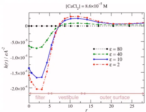
charge at that boundary. The distribution of the induced charge is shown in Fig. 11. The polarity of the induced charge indicates that the electric field crossing the boundary reverses polarity in the vestibular region near the pore as required by Gauss’s law that the total induced charge on the protein surface is zero 共see the sum rule discussed in Sec. III B 3兲.

Although the induced charge itself is small, the presence of the boundary with a weaker dielectric has a profound ef-fect: the number of cationic counterions attracted into the pore substantially increases as the dielectric coefficient of the protein is reduced共Fig.7兲. The local balance of ionic charge in the pore is thereby improved, and the field spreading from the pore into the protein is reduced. The small magnitude of the induced charge is the result of a strong negative feed-back: the electrostatic energy of the system would substan-tially increase if the ions in the pore created a significant electrical field across the weak dielectric of the protein.

The absorption of more ions into the pore is of potential physiological importance, because it allows the pore to use excluded volume to distinguish ions by size and thus to de-velop a selectivity for cations with larger valence or smaller size 共CSC mechanism16–18,20,21兲. Biological Ca channels have this kind of selectivity. Our simulations have used a pore model of rather large radius共4.5 Å兲. More narrow pore geometries are possible and might yield stronger selectivity. Simulations exploring this possibility will be presented in a later paper.

The analysis here uses a low-resolution representation of the dielectric properties of the protein and ionic solution. But it is important to remember that the physical phenomena described this way actually occur and must be visible and accurately computable if higher resolution simulations are to be more reliable than reduced models. In particular, induced charge will appear at any boundary separating materials in which electric fields move matter differently. High-resolution simulations must resolve such effects and compute them with calibrated accuracy as they extend and eventually replace the low-resolution methods used here.

V. SUMMARY

We describe a method to include dielectrics of complex geometry into MC simulations of charged systems. The ac-curacy of the method is verified, and the method is shown to be efficient for calculating the system’s electrostatic energy in every step of a simulation. The method is used to simulate a reduced model of ionic selectivity in biological Ca chan-nels.

Early theoretical studies of channels found that ions can-not cross an ion channel if the protein has a low dielectric coefficient because the ions induce repulsive surface charges on the dielectric interface.31–35 Here we find that the same physics can increasethe absorption of cations into the pore 共compared to having no dielectric interfaces兲if the channel pore contains negative charges from the protein; with a low protein dielectric coefficient, the negative protein charges in-duce negative surface charges on the dielectric interface that attract cations. Moreover, Ca2+ is preferentially absorbed over Na+, indicating the possibility that Ca channels use their dielectric properties to regulate their affinity for Ca2+.

ACKNOWLEDGMENTS

The authors are grateful for the support of the Hungarian National Research Fund 关OTKA K63322, to the authors 共D.B. and M.V.兲兴, NATO Grant No. PST.CLG.980366关to the authors 共D.H., D.G., and D.B.兲兴, and NIH Grant No. GM067241关to the authors共B.E. and D.G.兲兴. The use of the facilities of the Ira and Marylou Fulton Supercomputing Center at BYU is acknowledged with thanks.

1_{J. S. Smith, T. Imagawa, J. Ma, M. Fill, K. P. Campbell, and R.}

Coro-nado, J. Gen. Physiol. 92, 1共1988兲.

2_{W. A. Sather and E. W. McCleskey, Annu. Rev. Physiol. 65, 133共2003兲.}

3_{D. Gillespie, L. Xu, Y. Wang, and G. Meissner, J. Phys. Chem. B 109,}

15598共2005兲.

4_{M. Fill共private communication兲.}

5_{S. H. Heinemann, H. Terlau, W. Stuhmer, K. Imoto, and S. Numa, Nature}

共London兲 356, 441共1992兲.

6_{J. Yang, P. T. Ellinor, W. A. Sather, J. F. Zhang, and R. W. Tsien, Nature}

共London兲 366, 158共1993兲.

7_{P. T. Ellinor, J. Yang, W. A. Sather, J. F. Zhang, and R. W. Tsien, Neuron}

15, 1121共1995兲.

8_{L. Gao, D. Balshaw, L. Xu, A. Tripathy, C. Xin, and G. Meissner,}

Bio-phys. J. 79, 828共2000兲.

9_{Y. Wang, L. Xu, D. A. Pasek, D. Gillespie, and G. Meissner, Biophys. J.}

89, 256共2005兲.

10_{L. Xu, Y. Wang, D. Gillespie, and G. Meissner, Biophys. J. 90, 443}

共2006兲.

11_{C. K. Schauer and P. P. Anderson, J. Am. Chem. Soc.109, 3646共1987兲.}

12_{M. R. Nelson and W. J. Chazin, BioMetals 11, 297共1998兲.}

13_{http://structbio.vanderbilt.edu/cabp_database/cabp.html}

14_{B. Corry and S.-H. Chung, Cell. Mol. Life Sci. 63, 301共2006兲.}

15_{B. Corry, T. Vora, and S.-H. Chung, Biochim. Biophys. Acta 1711, 72}

共2005兲.

16_{D. Boda, D. Henderson, and D. D. Busath, Mol. Phys. 100, 2361共2002兲.}

17_{D. Boda, D. Henderson, and D. D. Busath, J. Phys. Chem. B 105, 11574}

共2001兲.

18_{W. Nonner, D. Gillespie, D. Henderson, and B. Eisenberg, J. Phys. Chem.}

B 105, 6427共2001兲.

19_{B. Corry, T. Allen, S. Kuyucak, and S.-H. Chung, Biophys. J. 80, 195}

共2001兲.

20_{D. Boda, D. D. Busath, D. Henderson, and S. Sokołowski, J. Phys. Chem.}

B 104, 8903共2000兲.

21_{W. Nonner, L. Catacuzzeno, and B. Eisenberg, Biophys. J. 79, 1976}

共2000兲. FIG. 11. 共Color online兲Distribution of induced charge on the protein

22_{W. Nonner and B. Eisenberg, Biophys. J. 75, 1287共1998兲.}

23_{M. Hoyles, S. Kuyucak, and S.-H. Chung, Phys. Rev. E 58, 3654共1998兲.}

24_{S.-H. Chung, M. Hoyles, T. Allen, and S. Kuyucak, Biophys. J. 75, 793}

共1998兲.

25_{R. Roth and D. Gillespie, Phys. Rev. Lett. 95, 054706共2005兲.}

26_{H. Miedema, A. Meter-Arkema, J. Wierenga, J. Tang, B. Eisenberg, W.}

Nonner, H. Hektor, D. Gillespie, and W. Meijberg, Biophys. J. 87, 3137 共2004兲.

27_{M. Vrouenraets, J. Wierenga, W. Meijberg, and H. Miedema, Biophys. J.}

90, 2102共2006兲.

28_{Z. S. Siwy, M. R. Powell, E. Kalman, R. D. Astumian, and R. S.}

Eisen-berg, Nano Lett. 6, 473共2006兲.

29_{D. Gillespie, W. Nonner, and R. S. Eisenberg, J. Phys.: Condens. Matter}

14, 12129共2002兲.

30_{D. Gillespie, W. Nonner, and R. S. Eisenberg, Phys. Rev. E 68, 031503}

共2003兲.

31_{V. A. Parsegian, Nature共London兲 221, 844共1969兲.}

32_{B. Neumcke and P. Läuger, Biophys. J. 9, 1160共1969兲.}

33_{D. G. Levitt, Biophys. J. 22, 209共1978兲.}

34_{D. G. Levitt, Biophys. J. 22, 221共1978兲.}

35_{P. C. Jordan, Biophys. J. 39, 157共1982兲.}

36_{D. Boda, D. Gillespie, W. Nonner, D. Henderson, and B. Eisenberg,}

Phys. Rev. E 69, 046702共2004兲.

37_{See EPAPS Document No. E-JCPSA6-125-514625 for description of}

sur-face disretization and figures on control simulations. This document can be reached via a direct link in the online article’s HTML reference section or via the EPAPS homepage共http://www.aip.org/pubservs/epaps.html兲. 38_{M. P. Allen and D. J. Tildesley,Computer Simulation of Liquids共Oxford,}

New York, 1987兲.

39_{D. Frenkel and B. Smit, Understanding Molecular Simulations 共}

Aca-demic, San Diego, 1996兲.

40_{R. J. Sadus,Molecular Simulation of Fluids; Theory, Algorithms, and}

Object-Orientation共Elsevier, Amsterdam, 1999兲.

41_{J. P. Valleau and L. K. Cohen, J. Chem. Phys. 72, 5935共1980兲.}

42_{D. Boda, D. Gillespie, B. Eisenberg, W. Nonner, and D. Henderson, in}

Ionic Soft Matter: Novel Trends in Theory and Applications, NATO Sci-ence Series: II: Mathematics, Physics and Chemistry, edited by D.

Hend-erson, M. Holovko, and A. Trokhymchuk共Springer, New York, 2005兲, Vol. 206.

43_{R. Allen, J.-P. Hansen, and S. Melchionna, Phys. Chem. Chem. Phys. 3,}

4117共2001兲.

44_{R. Allen, S. Melchionna, and J.-P. Hansen, Phys. Rev. Lett. 89, 175502}

共2002兲.

45_{R. Allen, S. Melchionna, and J.-P. Hansen, J. Phys.: Condens. Matter15,}

S297共2003兲.

46_{R. Allen, J.-P. Hansen, and S. Melchionna, J. Chem. Phys. 119, 3905}

共2003兲.

47_{S. Miertus, E. Scrocco, and J. Tomasi, Chem. Phys. 55, 117共1981兲.}

48_{J. Tomasi and M. Persico, Chem. Rev.共Washington, D.C.兲 94, 2027}

共1994兲.

49_{A. Klamt and G. Schüürmann, J. Chem. Soc., Perkin Trans. 1 2, 799}

共1993兲.

50_{B. Mennucci, E. Cancès, and J. Tomasi, J. Phys. Chem. B 101, 10506}

共1997兲.

51_{B. Mennucci and E. Cancès, J. Math. Chem. 23, 309共1998兲.}

52_{B. Mennucci, R. Cammi, and J. Tomasi, J. Chem. Phys. 109, 2798}

共1998兲.

53_{H. Hoshi, M. Sakurai, Y. Inoue, and R. Chûjô, J. Chem. Phys. 87, 1107}

共1987兲.

54_{R. Cammi and J. Tomasi, J. Chem. Phys. 100, 7495共1994兲.}

55_{R. Cammi and J. Tomasi, J. Chem. Phys. 101, 3888共1994兲.}

56_{C. S. Pomelli, J. Tomasi, and V. Barone, Theor. Chem. Acc. 105, 446}

共2001兲.

57_{L. Frediani, R. Cammi, S. Corni, and J. Tomasi, J. Chem. Phys. 120,}

3893共2004兲.

58_{M. E. Green and J. Lu, Prog. Colloid Polym. Sci. 171, 117共1997兲.}

59_{M. E. Green and J. Lu, J. Phys. Chem. B 101, 6512共1997兲.}

60_{J. Lu and M. E. Green, J. Phys. Chem. B 103, 2776共1999兲.}

61_{D. J. Griffiths, Introduction to Electrodynamics 共Prentice-Hall,}

Engle-wood Cliffs, 1999兲.

62_{M. Hoyles, S. Kuyucak, and S.-H. Chung, Comput. Phys. Commun. 115,}

45共1998兲.

63_{F. Chen and D. M. Chipman, J. Chem. Phys. 119, 10289共2003兲.}

Channel

Supplementary material

Dezs˝o Boda1,2∗_{, M´onika Valisk´o}2_{, Bob Eisenberg}1_{, Wolfgang Nonner}3_{, Douglas Henderson}4_{, Dirk Gillespie}1

1

Department of Molecular Biophysics and Physiology, Rush University Medical Center, Chicago, IL 60612 2

Department of Physical Chemistry, University of Veszpr´em, P.O. Box 158, H-8201 Veszpr´em, Hungary 3

Department of Physiology and Biophysics, University of Miami School of Medicine, Miami, FL 33101 and 4

Department of Chemistry and Biochemistry, Brigham Young University, Provo, UT 84602 (Dated: May 16, 2006)

Parametrization of the surface

Two-dimensional surfaces such as those used in this work can be parameterized using two variablest andφ. The transforms that converts these variables into Cartesian coordinates are

x=X(t, φ) y =Y(t, φ) z=Z(t, φ) (1)

and the corresponding area element is

A(t, φ) = s

_{∂(X, Y)} ∂(t, φ)

2 +

_{∂(Y, Z)} ∂(t, φ)

2 +

_{∂(Z, X)} ∂(t, φ)

2

(2)

where

∂(X, Y) ∂(t, φ) =

∂X ∂t ∂X ∂φ ∂Y ∂t ∂Y ∂φ (3)

The (outward) unit normal vector is

n(t, φ) =

_∂X ∂t , ∂Y ∂t , ∂Z ∂t × _∂X ∂φ, ∂Y ∂φ, ∂Z ∂φ _∂X ∂t , ∂Y ∂t , ∂Z ∂t × _∂X ∂φ, ∂Y ∂φ, ∂Z ∂φ (4)

If a portion of the surface is defined by theX,Y,Zfunctions over intervals [t1, t2] and [φ1, φ2], then these intervals are divided into Nt and Nφ subintervals {∆ti} and {∆φj}. The discretization of the [t1, t2] and [φ1, φ2] intervals does not have to be uniform; we can define smaller tiles in regions where we know that electric fields and/or the concentration of source charges is higher. For example, in the selectivity filter we use a fine grid with tile width about 1 ˚A, while far from the filter, at the outer surface of the protein we use tiles as large as 5 ˚A.

The center of area of tile (i, j) is defined as

¯ ti=

R R

(i,j)tA(t, φ)dtdφ R R

(i,j)A(t, φ)dtdφ

(5)

and similarly for ¯φj. The integrals are taken over the given tile. The integral of a vector fieldVanalogous to that in

the matrix then can be given as

Z

V(s−s∗_)·n(s)ds∗₌

Nt X i=1 Nφ X j=1

V(t, φ,¯t∗

i,φ¯∗j)·n(t, φ)A(¯t∗i,φ¯∗j)∆t∗i∆φ∗j (6)

where vectorsis parametrized by the parameterstandφ, while ¯t∗

i and ¯φ∗j are the centers of the tiles over which the

double sum runs.

The above description does not specify what is the surface over which the integral is taken. It can be a tile of the whole protein; in that case the above discretization is really a subdiscretization. The meaning of the variables can be different in various portions of the surface depending on its symmetry. For example, the model shown in Fig. 1 has a rotational symmetry: the surface of the protein is obtained as a surface of revolution about thez-axis. The formulas then can be simplified as

x=R(t) cosφ y=R(t) sinφ z=z(t) (7)

A(t, φ) =R(t) q

(z′_(t))2_{+ (R}′_(t))2 ₍₈₎

and

n(t, φ) = (z′(t) cosq φ, z′(t) sinφ,−R′(t)) (z′_(t))2_{+ (R}′_(t))2

(9)

(a)

20 A

60 A

ε=2

ε=2

ε=2

ε=80

ε=80

ε=80

ε=80

ε=2

(b)

40 60 80

c(

z)

0 0.05 0.1

c(

z)

0 0.05 0.1

0 1 2

c(

z)

0.05 0.1 0.15

0 5 10

z

3 6 9

c(

z)

10 20 30 40

z

0 0.001 0.002 0.003

O

1/2-Cl

-Na+

Ca2+

filter vestibule

Supplementary Figure 1The dielectric constant of the membrane was 80 in our simulations to save computer time

0 2 4 6 8

z

0 2 4 6 8

c(

z)

N_tiles=540

N_tiles=690

N_tiles=1462

0 10 20 30

r

h

S (r

)

A B

Ca

Na

r r

r

Supplementary Figure 2The longitudinal density profiles of Ca2+_{and Na}+ _{ions for varying resolution of the grid.}

The number of tiles 540, 690, and 1462 correspond to ∆x = 1.43, 1.25, and 0.84 ˚A, respectively, where ∆xis the width of the tiles in the filter. The simulations were performed forǫ= 10 and [CaCl2]=8.6×10−5M. The inset shows the distribution of the induced charge density along a path starting in the middle of the filter (point A) and ending in the middle of the outer bounding cylinder (point B). The surface charge is averaged over the angle of revolution and the two symmetric sides of the protein. The induced charge profile is the same for the two better resolutions, while it shows some deviation forNtiles= 540. The influence of the errors inh(r) on the ionic density profiles is negligible

40 60 80

N(Na+) = 200

N(Na+) = 300

N(Na+) = 400

0 0.05 0.1 0.15

0 0.05 0.1 0.15

0 3 6 9

0 0.05 0.1 0.15

0 5 10 15

z

3 6 9

10 20 30 40 50

z

0 0.0001 0.0002

O

Cl

-Na

Ca

filter vestibule bath ε = 10, [CaCl₂] = 8.7×10−5 M

c(

z)

0 0.5 1 1.5 2

0 0.5 1 1.5

Number of cations in the filter

-5 -4 -3 -2

0 0.5 1 1.5

-5 -4 -3 -2

Na

Ca

Na

Na

Na

Na

Na

Ca

Ca

Ca

Ca

Ca

ε = 80

ε = 40

ε = 20

ε = 10

ε = 5

ε = 2

lg[CaCl

] added to 0.1 M NaCl in bath

Supplementary Figure 4 The average numbers of Na+ _{and Ca}2+ _{ions with centers in specified regions of the}