Permanence, Almost Periodic Oscillations and Stability of Delayed Predator-Prey System with General Functional Response

(1)

Permanence, Almost Periodic Oscillations and

Stability of Delayed Predator-Prey System with

General Functional Response

Ting Yuan, Liyan Pang and Tianwei Zhang

Abstract—By using some new analytical techniques and Mawhin’s continuous theorem of coincidence degree theory, some new sufficient conditions for the existence of positive almost periodic solutions to a class of predator-prey system with general functional response and time delays are estab-lished. Secondly, by using the comparison theorem, we give a permanence result for the model. By using the Lyapunov method of differential equations, sufficient conditions which guarantee uniform asymptotical stability of the model are obtained. Finally, two examples and simulations are given to illustrate the main result of this paper.

Index Terms—Almost periodic oscillation; Coincidence de-gree; Predator-prey; Functional response.

I. INTRODUCTION

I

T is well-known that the theoretical study of predator-prey systems in mathematical ecology has a long history starting with the pioneering work of Lotka and Volterra [1-2]. The principles of Lotka-Volterra model, conservation of mass and decomposition of the rates of change in birth and death processes, have remained valid until today and many theoretical ecologists adhere to these principles. This general approach has been applied to many biological systems in particular with functional response. In population dynamics, a functional response of the predator to the prey density refers to the change in the density of prey attached per unit time per predator as the prey density changes. During the last ten years, there has been extensively investigation on the dynamics of predator-prey models with the differ-ent functional responses in the literature, (see [1-15] and references therein). In particular, the existence of positive periodic solutions of the predator-prey system with some monotone or non-monotone functional responses has been studied extensively in the literature.

In [7], Wang and Li considered the following system with

Manuscript received June 4, 2018; revised December 10, 2018. Ting Yuan is with the Department of Basic Education, Yunnan College of Tourism Vocation, Kunming 650221, China. ([email protected]).

Liyan Pang is with the School of Mathematics and Computer Science, Ningxia Normal University, Guyuan, Ningxia 756000, China. ([email protected]).

Tianwei Zhang is with the City College, Kunming University of Science and Technology, Kunming 650051, China. ([email protected]).

Correspondence author: Tianwei Zhang. ([email protected]).

Holling III type functional response:



          

          

˙

N1(t) = N1(t)

b1(t)−a1(t)N1(t−µ1(t))

−α1(t)N1(t)

1+mN2 1(t)

N2(t−ν(t))

,

˙

N2(t) = N2(t)

−b2(t)−a2(t)N2(t)

+α2(t)N12(t−µ3(t))

1+mN2

1(t−µ3(t))

.

(1.1)

Xu et al. [9] studied the following system with Holling II type functional response:



          

          

˙

N1(t) = N1(t)

b1(t)−a1(t)N1(t−µ1(t))

−α1(t)N1(t)

1+mN1(t)N2(t)

,

˙

N2(t) = N2(t)

−b2(t)−a2(t)N2(t−µ2(t))

+α2(t)N1(t−µ3(t))

1+mN1(t−µ3(t))

.

(1.2)

By using Mawhin’s continuation theorem of coincidence degree theory, the authors [7, 9] obtained sufficient conditions which guarantee the existence of positive periodic solution of systems (1.1)-(1.2).

However, in real world phenomenon, if the various con-stituent components of the temporally nonuniform environ-ment is with incommensurable (nonintegral multiples, see Example 1) periods, then one has to consider the environ-ment to be almost periodic [10] since there is no a priori reason to expect the existence of periodic solutions. Hence, if we consider the effects of the environmental factors, almost periodicity is sometimes more realistic and more general than periodicity.

Example 1. Let us consider the following simple population

model:

˙

N(t) =N(t)h|sin(√2t)| − |sin(√3t)|N(t)i. (1.3)

In Eq. (1.3), |sin(√2t)| is

√

2π

2 -periodic function and

|sin(√3t)| is

√

3π

3 -periodic function, which imply that

E-q. (1.3) is with incommensurable periods. Then there is no a priori reason to expect the existence of positive periodic solutions of Eq. (1.3). Thus, it is significant to study the existence of positive almost periodic solutions of Eq. (1.3).

In view of this, now we consider the following almost pe-riodic predator-prey system with general functional response

IAENG International Journal of Applied Mathematics, 49:2, IJAM_49_2_03

(2)

and time delays:



          

          

˙

N1(t) = N1(t)

b1(t)−a1(t)N

q1

1 (t−µ1(t))

−α1(t)N1p−1(t)

1+mN₁p(t) N2(t−ν(t))

,

˙

N2(t) = N2(t)

−b2(t)−a2(t)N2q2(t−µ2(t))

+α2(t)N1p(t−µ3(t))

1+mN₁p(t−µ3(t))

,

(1.4)

whereN1 andN2 represent the densities of the prey

popu-lation and predator popupopu-lation, respectively, p is a positive constant and p ≥ 1, m is a nonnegative constant and q1, q2 are positive constants. From systems (1.1)-(1.2), we

know that the prey population and predator population obey the logistic growth. But many authors have suspected the reasonableness of the logistic equations [16,17]. Hence, some of them proposed single growth population models in succession, such as Gilpin model [16], Smith model [17] etc. Therefore, we consider system (1.4), which are more general and reasonable. Let R, Z and N+ denote the sets of real numbers, integers and positive integers, respectively. Related to a continuous function f, we use the following notations:

fl= inf s∈R

f(s), fM = sup s∈R

f(s),

|f|∞= sup

s∈R

|f(s)|, f¯= lim T→∞

1 T

Z T

0

f(s) ds.

Throughout this paper, we always make the following assumption for system (1.4):

(F1) All the coefficients of system (1.4) are nonnegative

almost periodic functions with ¯ai > 0 and ¯b1 > 0,

i= 1,2.

The initial conditions of system (1.4) are of the form

Ni(s) =ψi(s), s∈[−µ,0], ψi(0)>0,

ψi∈C([−µ,0],[0,+∞)), i= 1,2,

whereµ:= maxi=1,2,3{µMi , ν M_}_.

It is well known that Mawhin’s continuation theorem of coincidence degree theory is an important method to investigate the existence of positive periodic solutions of some kinds of non-linear ecosystems (see [7-14]). However, it is difficult to be used to investigate the existence of positive almost periodic solutions of non-linear ecosystems. Therefore, to the best of the author’s knowledge, so far, there are scarcely any papers concerning with the existence of positive almost periodic solutions of system (1.4). Motivated by the above reason, the main purpose of this paper is to establish some new sufficient conditions on the existence of positive almost periodic solutions of system (1.4) by using Mawhin’s continuous theorem of coincidence degree theory. The paper is organized as follows. In Section 2, we give some basic definitions and necessary lemmas which will be used in later sections. In Section 3, we obtain some new sufficient conditions for the existence of at least one positive almost periodic solution of system (1.4) by way of Mawhin’s continuous theorem of coincidence degree

theory. Two illustrative examples and simulations are given in Section 4.

II. PRELIMINARIES

Definition 1. ([18,19]) x ∈ C(R,Rn) is called almost

periodic, if for any > 0, it is possible to find a real number l = l() > 0, for any interval with length l(), there exists a number τ = τ() in this interval such that

kx(t+τ)−x(t)k < , ∀t ∈ R, where k · k is arbitrary norm ofRn.τ is called to the-almost period ofx,T(x, ) denotes the set of -almost periods for xand l() is called to the length of the inclusion interval for T(x, ). The collection of those functions is denoted byAP(_R,_Rn₎_{. Let} AP(_R) :=AP(_R,_R).

Lemma 1. ([18,19])Ifx∈AP(_R), thenxis bounded and

uniformly continuous onR.

Lemma 2. ([18,19]) If x ∈ AP(R), then R0tx(s) ds ∈

AP(_R)if and only if R₀tx(s) dsis bounded onR.

Lemma 3. ([21]) Assume thatx∈AP(_R)∩C1₍

R) with

˙

x∈C(R). For arbitrary interval[a, b]withb−a=ω >0,

letξ, η∈[a, b] and

I=

s∈[ξ, b] : ˙x(s)≥0 , J =

s∈[a, η] : ˙x(s)≥0 ,

then ones have

x(t)≤x(ξ) +

Z

I ˙

x(s) ds, ∀t∈[ξ, b],

x(t)≥x(η)− Z

J ˙

x(s) ds, ∀t∈[a, η].

Lemma 4. ([21])Ifx∈AP(R), then for arbitrary interval

[a, b]withb−a=ω >0, there existξ∈[a, b],ξ∈(−∞, a]

andξ¯∈[b,+∞)such that

x(ξ) =x( ¯ξ) and x(ξ)≤x(s), ∀s∈[ξ,ξ¯].

Lemma 5. ([21])Ifx∈AP(R), then for arbitrary interval

[a, b] with I =b−a =ω > 0, there exist η ∈ [a, b], η ∈ (−∞, a]and η¯∈[b,+∞)such that

x(η) =x(¯η) and x(η)≥x(s), ∀s∈[η,η¯].

Lemma 6. ( [21]) If x ∈ AP(R), then for ∀n ∈ N+,

there exist αn, βn ∈ R such that x(αn) ∈ x∗−n1, x

∗

and x(βn) ∈

x∗, x∗+n1

, where x∗ = sup_s_∈_Rx(s) and

x∗= infs∈Rx(s).

Forx∈AP(R), we denote by

¯

x=m(x) = lim T→∞

1 T

Z T

0

x(s) ds,

a(x, $) = lim T→∞

1 T

Z T

0

x(s)e−i$sds,

Λ(x) =

$∈_R: lim T→∞

1 T

Z T

0

x(s)e−i$sds6= 0

the mean value and the set of Fourier exponents of x, respectively.

Lemma 7. ([21])Assume thatx∈AP(R)andx >¯ 0, then

for∀t0∈R, there exists a positive constantT0independent

IAENG International Journal of Applied Mathematics, 49:2, IJAM_49_2_03

(3)

oft0 such that

1 T

Z t0+T

t0

x(s) ds∈ _¯_x

2, 3¯x

2

, ∀T ≥T0.

The method to be used in this paper involves the appli-cations of the continuation theorem of coincidence degree. This requires us to introduce a few concepts and results from Gaines and Mawhin ([20]).

Mawhin’s Continuous Theorem. ([20])LetΩ⊆Xbe an

open bounded set, Lbe a Fredholm mapping of index zero and N be L-compact onΩ¯. If all the following conditions hold:

(a) Lx6=λN x,∀x∈∂Ω∩DomL, λ∈(0,1); (b) QN x6= 0,∀x∈∂Ω∩KerL;

(c) deg{J QN,Ω∩KerL,0} 6= 0,whereJ : ImQ→KerL

is an isomorphism.

ThenLx=N xhas a solution on Ω¯ ∩DomL.

Under the invariant transformation (N1, N2)T =

(eu, ev)T, system (1.4) reduces to



   

   

˙

u(t) = b1(t)−a1(t)eq1u(t−µ1(t))

−α1(t)e(p−1)u(t)

1+mepu(t) e

v(t−ν(t))_,

˙

v(t) = −b2(t)−a2(t)eq2v(t−µ2(t))

+α2(t)epu(t−µ3 (t))

1+mepu(t−µ3 (t)).

(2.1)

SetX=Y=V1LV2, where

V1=

z= (u, v)T ∈AP(_R,_R2) :

∀$∈Λ(u)∪Λ(v),|$| ≥γ0

,

V2=z= (u, v)T ≡(k1, k2)T, k1, k2∈R ,

whereγ0 is a given positive constant. Define the norm

kzk_X= max

sup s∈R

|u(s)|,sup s∈R

|v(s)|

, ∀z∈X=Y.

Lemma 8. ( [21])Let x∈ AP(R). For ∀$ ∈Λ(x) with

|$| ≥γ0>0, then

Rt

0x(s) ds∈AP(R).

Lemma 9. ( [21]) Let f ∈ AP(_R) such that f(t) _∼

P_a₍_{f, λn}₎_eiλnt_with_|_λn_{| ≥}_γ

0>0. Ifgis the integral off

witha(g,0) = 0, then there exists a constantD independent off,g andγ0 such that|g|∞≤D|f|∞.

Lemma 10. ([21]) Xand Y are Banach spaces endowed

withk · k_X.

Lemma 11. ( [21]) Let L : _X → Y, Lz = L(u, v)T =

( ˙u,v˙)T_{, then}_L _{is a Fredholm mapping of index zero.}

Lemma 12. ( [21]) Define N : X→ Y,P : X→ Xand

Q:Y→Yby

N z=N

u v

=



   

b1(t)−a1(t)eq1u(t−µ1(t))

−α1(t)e(p−1)u(t)

1+mepu(t) e v(t−ν(t))

−b2(t)−a2(t)eq2v(t−µ2(t))

1+mepu(t−µ3 (t))



   

,

P z=P

u v

=

m(u) m(v)

=Qz, ∀z∈_X=_Y.

ThenN isL-compact onΩ(Ω¯ is an open and bounded subset ofX).

III. MAIN RESULTS

Now we are in the position to present and prove our result on the existence of at least one positive almost periodic solution for system (1.4).

Take

l0:= max{sup

s∈R

µ1(s),sup

s∈R

µ2(s)}.

From (F1) and Lemma 7, for ∀k ∈ R, there exists a constantω0∈(2l0,+∞)independent ofksuch that

1 T

Z k+T

k

ai(s) ds∈

¯ ai

2, 3¯ai

2

,

1 T

Z k+T

k

b1(s) ds∈

¯_b

1

2, 3¯b1

2

, (3.1)

where∀T ≥ω0

2, i= 1,2.

Let

ρ1:= ln

6¯b1

¯ a1

_q1

1

+bM₁ ω0,

ρ2:= ln

₄_αM

2 e

pρ1 (1 +mepρ1_)¯_a

2

q12 +α

M

2 e

pρ1_ω

0

1 +mepρ1.

Therefore, we may introduce a assumption as follows:

(F2) ¯Φ1 := lim

T→+∞

1 T

Z T

0

b1(s)−e(p−1)ρ1+ρ2α1(s)

ds >

0.

Similar to(3.1), for∀k∈_R, there exists a constant τ0∈

(ω0,+∞)independent ofksuch that

1 T

Z k+T

k

Φ1(s) ds∈

_¯

Φ1

2 , 3 ¯Φ1

2

, ∀T ≥τ0. (3.2)

Theorem 1. Assume that (F1), (F2) and the following

condition hold:

(F3) ¯Φ2 := lim

T→+∞

1 T

Z T

0

_epρ3

1 +mepρ3α2(s)−b2(s)

ds >

0, where

ρ3:= ln

_Φ_¯

1

4aM

1

q1₁

−bM1 π0,

π0:= max

τ0,

4aM

1 eq1ρ1l0

¯ Φ1

.

Then system (1.4) admits at least one positive almost peri-odic solution.

Proof: It is easy to see that if system (2.1) has one

almost periodic solution(¯u,v¯)T_{, then}_{( ¯}_N

1,N¯2)T=(eu¯, ev¯)T

is a positive almost periodic solution of system (1.4). There-fore, to complete the proof it suffices to show that system (2.1) has one almost periodic solution.

In order to use the Mawhin’s continuous theorem, we set the Banach spaces _X and _Y as those in Lemma 10 and L, N, P, Q the same as those defined in Lemmas 11 and 12, respectively. It remains to search for an appropriate open and bounded subsetΩ⊆X.

Corresponding to the operator equation Lz = λz, λ ∈

IAENG International Journal of Applied Mathematics, 49:2, IJAM_49_2_03

(4)

(0,1), we have



          

          

˙

u(t) = λ

b1(t)−a1(t)eq1u(t−µ1(t))

−α1(t)e(p−1)u(t)

1+mepu(t) e v(t−ν(t))

,

˙

v(t) = λ

−b2(t)−a2(t)eq2v(t−µ2(t))

1+mepu(t−µ_{3 (}t))

.

(3.3)

Suppose that(u, v)T _∈_Dom_L_⊆

Xis a solution of system (3.3) for some λ∈(0,1), where DomL={z = (u, v)T _∈ X: u, v ∈ C1(R),u,˙ v˙ ∈ C(R)}. By Lemma 6, there exist two sequences{Tn:n∈N+}and{Pn:n∈N+}such that

u(Tn)∈

u∗−1

n, u

∗

, u∗= sup s∈R

u(s), n∈N+,(3.4)

v(Pn)∈

v∗− 1

n, v

∗

, v∗= sup s∈R

v(s), n∈_N+_.(3.5)

For ∀n0 ∈N+, we consider [Tn0 −ω0, Tn0] and [Pn0− ω0, Pn0], whereω0 is defined as that in (3.1). By Lemma

4, there existξ∈[Tn₀−ω0, Tn0],ξ∈(−∞, Tn0−ω0]and ¯

ξ∈[Tn0,+∞)such that

u(ξ) =u( ¯ξ) and u(ξ)≤u(s), ∀s∈[ ¯ξ, ξ]. (3.6)

Integrating the first equation of system (3.3) fromξtoξ¯leads to

Z ξ¯

ξ

b1(s)−a1(s)eq1u(s−µ1(s))

−α1(s)e

(p−1)u(s)

1 +mepu(s) e

v(s−ν(s))

ds= 0,

which yields that

Z ξ¯

ξ+l0

a1(s)eq1u(s−µ1(s))ds≤

Z ξ¯

ξ

a1(s)eq1u(s−µ1(s))ds

≤ Z ξ¯

ξ

b1(s) ds.

By the integral mean value theorem and (3.1), there exists s0∈[ξ+l0,ξ¯] (s0−µ1(s0)∈[ξ,ξ¯])such that

¯ a1

4e

q1u(s0−µ1(s0))

≤ ¯

ξ−ξ−l0

¯ ξ−ξ

¯ a1

2 e

q1u(s0−µ1(s0))

≤ ¯

ξ−ξ−l0

¯ ξ−ξ e

q1u(s0−µ1(s0)) 1

¯

ξ−ξ−l0

Z ξ¯

ξ+l0

a1(s) ds

= _¯1 ξ−ξ

Z ξ¯

ξ+l0

≤ _¯1

ξ−ξ

Z ξ¯

ξ

b1(s) ds

≤ 3¯b1 2 ,

which implies from(3.6) that

u(ξ)≤ln

_6¯_b

1

¯ a1

q11

. (3.7)

LetI1={s∈[ξ, Tn0] : ˙u(s)≥0}. It follows from system (3.3) that

Z

I1 ˙

u(s) ds =

Z

I1 λ

−α1(s)e

(p−1)u(s)

1 +mepu(s) e

v(s−ν(s))

ds

≤ Z

I1

λb1(s) ds≤

Z Tn0

Tn0−ω0

b1(s) ds

≤ bM₁ ω0. (3.8)

By Lemma 3, it follows from (3.7)-(3.8) that

u(t)≤u(ξ) +

Z

I1 ˙

u(s) ds≤ln

_6¯_b

1

¯ a1

q11

+bM₁ ω0:=ρ1,

∀t∈[ξ, Tn0], which implies that

u(Tn0)≤ρ1.

In view of (3.4), lettingn0 →+∞in the above inequality

leads to

u∗= lim

n0→+∞u(Tn0)≤ρ1. (3.9)

Also, by Lemma 4, there exist ζ∈[Pn0 −ω0, Pn0], ζ∈ (−∞, Pn₀−ω0]andζ¯∈[Pn0,+∞)such that

v(ζ) =v( ¯ζ) and v(ζ)≤v(s), ∀s∈[ζ,ζ¯]. (3.10)

Integrating the second equation of system (3.3) fromζ toζ¯ leads to

Z ζ¯

ζ

−b2(s)−a2(s)eq2v(s−µ2(s))

+α2(s)e

pu(s−µ3(s)) 1 +mepu(s−µ3(s))

ds= 0, (3.11)

which yields that

Z ζ¯

ζ+l0

a2(s)eq2v(s−µ2(s))ds≤

Z ζ¯

ζ

a2(s)eq2v(s−µ2(s))ds

≤ Z ζ¯

ζ

α2(s)epu(s−µ3(s))

1 +mepu(s−µ3(s))ds.

By a similar argument as that in (3.7), there exists c0 ∈

[ζ+l0,ζ¯] (c0−µ2(c0)∈[ζ,ζ¯])such that

¯ a2

4 e

q2v(c0−µ2(c0)) _≤ 1 ¯ ζ−ζ

Z ζ¯

ζ+l0

≤ _¯1

ζ−ζ

Z ζ¯

ζ

1 +mepu(s−µ3(s)) ds

≤ α

M

2 e

pρ1 1 +mepρ1, which implies from(3.10)that

v(ζ)≤ln

₄_αM

2 epρ1

(1 +mepρ1_)¯_a₂

q12

. (3.12)

IAENG International Journal of Applied Mathematics, 49:2, IJAM_49_2_03

(5)

LetI2={s∈[ζ, Pn0] : ˙v(s)≥0}. It follows from system (3.3) that

Z

I2 ˙

v(s) ds =

Z

I2 λ

+α2(s)e

pu(s−µ3(s)) 1 +mepu(s−µ3(s))

ds

≤ Z

I2

λα2(s)e

pu(s−µ3(s)) 1 +mepu(s−µ3(s)) ds

≤ Z Pn0

Pn₀−ω0

1 +mepu(s−µ3(s))ds

≤ α

M

2 epρ1ω0

1 +mepρ1. (3.13)

v(t) ≤ v(ζ) +

Z

I2 ˙ v(s) ds

≤ ln

₄_αM

2 epρ1

(1 +mepρ1_)¯_a₂

q12 +α

M

2 epρ1ω0

1 +mepρ1 := ρ2, ∀t∈[ζ, Pn0],

which implies that

v(Pn0)≤ρ2.

In view of (3.5), letting n0 →+∞ in the above inequality

leads to

v∗= lim n0→+∞

v(Pn0)≤ρ2. (3.14)

On the other hand, by Lemma 6, there exists a sequence

{Hn:n∈_N+_}_{such that}

u(Hn)∈

u∗, u∗+

1 n

, u∗= inf

s∈R

u(s), n∈N+.(3.15)

For ∀n0 ∈ N+, we consider [Hn0, Hn0 +π0]. By Lemma 4, there exist η ∈ [Hn₀, Hn₀ +π0], η ∈ (−∞, Hn0] and ¯

η∈[Hn₀,+∞)such that

u(η) =u(¯η) and u(η)≥u(s), ∀s∈[η,η¯]. (3.16)

Integrating the first equation of system (3.3) from η to η¯ leads to

Z η¯

η

−α1(s)e

(p−1)u(s)

1 +mepu(s) e

v(s−ν(s))

ds= 0, (3.17)

which yields from (3.9) and (3.14) that

Z η¯

η

b1(s)−α1(s)e(p−1)ρ1eρ2ds

≤ Z η¯

η

b1(s)−

α1(s)e(p−1)u(s)

1 +mepu(s) e

v(s−ν(s))

ds

=

Z η¯

η

=

Z η¯

η+l0

+

Z η+l0

η

≤ Z η¯

η+l0

a1(s)eq1u(s−µ1(s))ds+aM1 e

q1ρ1_l

0,

which implies from(3.2) that ¯

Φ1

2 ≤

1 ¯ η−η

Z η¯

η

b1(s)−α1(s)e(p−1)ρ1eρ2ds

≤ 1

¯ η−η

Z η¯

η+l0

a1(s)eq1u(s−µ1(s))ds+

aM

1 eq1ρ1l0

¯ η−η

≤ 1

¯ η−η

Z η¯

η+l0

aM1 eq1ρ1l0

π0

≤ 1

¯ η−η

Z η¯

η+l0

¯ Φ1

4 . (3.18)

In view of (3.18), by the integral mean value theorem and (3.16), there exists s1 ∈ [η+l0,η¯] (s1−µ1(s1) ∈ [η,η¯])

such that ¯ Φ1

4 ≤

eq1u(s1−µ1(s1))

¯ η−η

Z η¯

η+l0

a1(s) ds

≤aM₁ eq1u(η)η¯−η−l0 ¯

η−η ≤a M

1 e

q1u(η)_, _(3.19)

which implies that

u(η)≥ln

_Φ¯

1

4aM

1

q11

. (3.20)

LetJ ={s∈[Hn0, η] : ˙u(s)≥0}. It follows from system (3.3) that

Z

J ˙

u(s) ds =

Z

J λ

−α1(s)e

(p−1)u(s)

1 +mepu(s) e

v(s−ν(s))

ds

≤ Z

J

λb1(s) ds≤

Z Hn0+π0 Hn₀

b1(s) ds

≤bM₁ π0. (3.21)

u(t)≥u(η)− Z

J ˙

u(s) ds≥ln

_Φ_¯

1

4aM

1

q11

−bM₁ π0

:=ρ3, ∀t∈[Hn0, η],(3.22)

which implies that

u(Hn₀)≥ρ3.

In view of (3.16), lettingn0→+∞in the above inequality

leads to

u∗= lim

n0→+∞u(Hn0)≥ρ3. (3.23) Take

σ1:= max

π0,

4aM₂ eq2ρ2_l

0

¯ Φ2

.

From(F3)and Lemma 7, for∀k∈R, there exists a constant σ0∈(σ1,+∞)independent ofksuch that

1 T

Z k+T

k

Φ2(s) ds∈

_Φ¯

2

2 , 3 ¯Φ2

2

, ∀T ≥σ0. (3.24)

Also, there exist ς ∈ [n0σ0, n0σ0 +σ0](∀n0 ∈ Z), ς ∈

IAENG International Journal of Applied Mathematics, 49:2, IJAM_49_2_03

(6)

(−∞, n0σ0] andς¯∈[n0σ0+σ0,+∞)such that

v(ς) =v(¯ς) and v(ς)≥v(s), ∀s∈[ς,ς¯]. (3.25)

Integrating the second equation of system (3.3) from ς toς¯ leads to

Z ς¯

ς

+α2(s)e

pu(s−µ3(s))

1 +mepu(s−µ3(s))

ds= 0,

which yields that

Z ¯ς

ς

epρ3

1 +mepρ3α2(s)−b2(s)

ds

≤ Z ¯ς

ς

−b2(s) +

1 +mepu(s−µ3(s))

ds

=

Z ¯ς

ς

=

Z ¯ς

ς+l0

+

Z ς+l0

ς

≤ Z ¯ς

ς+l0

a2(s)eq2v(s−µ2(s))ds+aM2 e

q2ρ2_l

0.

Similar to the argument as that in (3.18), we obtain that ¯

Φ2

2 ≤ 1 ¯ ς−ς

Z ς¯

ς+l0

a2(s)eq2v(s−µ2(s))ds+

¯ Φ2

4 . (3.26)

In view of (3.24), by the integral mean value theorem and (3.23), there existsc1∈[ς+l0,ς¯] (c1−µ2(c1)∈[ς,ς¯])such

that

¯ Φ2

4 ≤

eq2v(c1−µ2(c1)) ¯

ς−ς

Z ¯ς

ς+l0

a2(s) ds

≤aM₂ eq2v(ς)¯ς−ς−l0 ¯ ς−ς

≤aM₂ eq2v(ς)_,

which implies that

v(ς)≥ln

_Φ¯

2

4aM

2

q12

. (3.27)

Further, we obtain from system (3.3) that

Z n0σ0+σ0 n0σ0

|v˙(s)|ds

=

Z n0σ0+σ0

n0σ0 λ

+α2(s)e

pu(s−µ3(s))

1 +mepu(s−µ3(s))

ds

≤[bM₂ +a₂Meq2ρ2₊_αM

2 e

pρ1_]_σ

0:= Θ2. (3.28)

It follows from (3.25)-(3.26) that

v(t) ≥ v(ς)−

Z n0σ0+σ0

n0σ0

|v˙(s)|ds

≥ ln

_Φ_¯

2

4aM

2

q1₂

−Θ2

:= ρ4, ∀t∈[n0σ0, n0σ0+σ0]. (3.29)

Obviously,ρ4 is a constant independent ofn0. So it follows

from (3.27) that

v∗= inf

s∈R

v(s) = inf n0∈Z

min s∈[n0σ0,n0σ0+σ0]

v(s)

≥ inf n0∈Z

{ρ4}=ρ4. (3.30)

Set K = |ρ1| +|ρ2|+|ρ3|+|ρ4| + 1, then kzkX =

k(u, v)T_k _{< K. Clearly,} _K _{is independent of} _λ _∈ ₍₀_,₁₎_. Consider the algebraic equations QN z0 = 0 for z0 =

(u0_{, v}0₎T _∈

R2 as follows:







0 = ¯b1−¯a1eq1u

0

−α¯1e(p−1)u 0

1+mepu0 e v0

,

0 = −¯b2−a¯2eq2v

0

+ α¯2epu 0

1+mepu0.

Similar to the arguments as that in (3.9), (3.14), (3.21) and (3.28), we can easily obtain that

ρ3≤u0≤ρ1, ρ4≤v0≤ρ2.

Thenkz0kX=|u0|+|v0|< K. Let Ω ={z ∈X:kzkX<

K}, then Ω satisfies conditions (a) and (b) of Mawhin’s continuous theorem.

Finally, we will show that condition (c) of Mawhin’s continuous theorem is satisfied. Let us consider the homotopy

H(ι, z) =ιQN z+ (1−ι)F z, (ι, z)∈[0,1]×R2,

where

F z=F

u v

=

¯_b

1−¯a1eq1u

−¯b2−¯a2eq2v+ α2e¯ pu

1+mepu

.

From the above discussion it is easy to verify thatH(ι, z)6= 0 on ∂Ω∩KerL. By the invariance property of homotopy, we have

deg J QN,Ω∩KerL,0

= deg QN,Ω∩KerL,0

= deg F,Ω∩KerL,0

,

wheredeg(·,·,·)is the Brouwer degree andJ is the identity mapping sinceImQ= KerL.

Note that the equations of the following system

¯_b

1−¯a1eq1u= 0,

−¯b2−¯a2eq2v+ α2e¯ pu

1+mepu = 0

has a solution:

(u∗, v∗) =

ln

¯_b

1

¯ a1

q11 ,ln

α2e¯

pu∗ 1+mepu∗ −¯b2

¯ a2

q12

∈Ω.

It follows that

deg J QN,Ω∩KerL,0

= deg F,Ω∩KerL,0

= sign

−q1¯a1eq1u 0

d du

_α_¯

2epu

1 +mepu

−q2¯a2eq2v

₍_u,v₎₌₍_u∗_,v∗₎

= sign eq1u∗_eq2v∗ = 1.

Obviously, all the conditions of Mawhin’s continuous theorem are satisfied. Therefore, system (2.1) has one almost periodic solution, that is, system (1.4) has at least one

IAENG International Journal of Applied Mathematics, 49:2, IJAM_49_2_03

(7)

positive almost periodic solution. This completes the proof.

Theorem 2. Assume that(F1)and the following conditions

hold:

(F4) p >1 +mepρ1.

(F5) ¯Ψ1:= lim

T→+∞

1 T

Z T

0

b1(s)−

e(p−1)ρ1+ρ2 1 +mepρ1 α1(s)

ds >

0.

(F6) ¯Ψ2 := lim

T→+∞

1 T

Z T

0

_epρ3˜

1 +mepρ˜3α2(s)−b2(s)

ds >

0, where

˜ ρ3:= ln

_Ψ¯

1

4aM

1

q11

−bM₁ ˜π0,

˜

π0:= max

τ0,

4aM1 eq1ρ1l0

¯ Ψ1

.

Then system (1.4)admits at least one positive almost peri-odic solution.

Proof: Let

L(x) = x p−1

1 +mxp, ∀x∈(0, e ρ1_]_.

By (F4), we are easily obtain that

˙

L(x) = x

p−2₍_p₋₁₋_mxp₎

(1 +mxp₎2 >0, ∀x∈(0, e

ρ1_]_,

which implies that

max

x∈(0,eρ1]L(x) =

e(p−1)ρ1

1 +mepρ1. (3.31)

By the same arguments as that in Theorem 1, we have (3.10), (3.15)-(3.18). In view of (3.18), it follows from (3.10), (3.15) and (3.30) that

¯ Ψ1

2 ≤

1 ¯ η−η

Z η¯

η

b1(s)−α1(s)

e(p−1)ρ1+ρ2 1 +mepρ1

ds

≤ 1

¯ η−η

Z η¯

η

b1(s)−

α1(s)e(p−1)u(s)

1 +mepu(s) e

v(s−ν(s))

ds

=

Z η¯

η

≤ 1

¯ η−η

Z η¯

η+l0

¯ Ψ1

4 .

Similar to the argument as that in (3.20), we have

u(η)≥ln

_¯

Ψ1

4aM

1

_q1

1 .

The remaining proof is similar to Theorem 1, so we omit it. This completes the proof.

From the proves of Theorems 1-2, we can show that

Corollary 1. Assume that (F1)-(F3) hold. Suppose further

thatai,bi,αi,µjandνare continuous nonnegative periodic functions with different periods, i = 1,2, j = 1,2,3, then system (1.1) admits at least one positive almost periodic solution.

Remark 1. By Corollary 1, it is easy to obtain the existence

of at least one positive almost periodic solution of Eq. (1.3) in Example 1, although there is no a priori reason to expect the existence of positive periodic solutions of Eq. (1.3).

Corollary 2. Assume that (F1), (F4)-(F6) hold. Suppose

further thatai,bi,αi,µj and ν are continuous nonnegative

periodic functions with different periods,i= 1,2,j= 1,2,3, then system(1.1)admits at least one positive almost periodic solution.

Assume that all coefficients of system (1.4) areω-periodic functions, let

ˆ ρ1:= ln

¯_b

1

¯ a1

q11 + ¯b1ω,

ˆ ρ2:= ln

_αu

2epρ1ˆ

(1 +mepρˆ1)¯a₂

q12

+ min

( ¯B2+ ¯b2)ω,

¯ α2epρˆ1ω

1 +mepρ1ˆ

.

From the proves of Theorems 1-2, we can show that

Corollary 3. Assume that(F1)and the following conditions

hold:

(F7) ¯b1> e(p−1) ˆρ1+ ˆρ2α¯1,

(F8) epρˆ3α¯2>(1 +mepρˆ3)¯b2, where

ˆ ρ3:= ln

¯_b

1−e(p−1) ˆρ1+ ˆρ2α¯1

¯ a1

q11

−¯b1ω.

Then system (1.4) admits at least one positive ω-periodic solution.

Corollary 4. Assume that(F1)and the following conditions

hold:

(F9) p >1 +mepρˆ1,

(F10) (1 +mepρˆ1)¯b1> e(p−1) ˆρ1+ ˆρ2α¯1,

(F11) ep~ρ3α¯2>(1 +mep~ρ3)¯b2, where

~ ρ3:= ln

¯_b

1−e

(p−1) ˆρ1 + ˆρ2

1+mepρˆ1 α¯1 ¯

a1

q11

−¯b1ω.

Then system (1.4) admits at least one positive ω-periodic solution.

IV. Uniform persistence

Our object in this section is to prove the uniform persis-tence of system (1.4).

Theorem 3. Let p=q1=q2 = 1 in system (1.4). Assume

that

(H1) b−1 > α +

1M2,(1 +mM1)−1α−2N1> b+2,

then for any positive solution (N1, N2)T of system (1.4)

satisfies

Ni≤Ni(t)≤Mi, i= 1,2,

where Ni and Mi are defined as those in (4.1)-(4.4), i = 1,2,3. That is, system (1.4) is uniformly persistent.

Proof: We have from the first equation of system (1.4)

that

˙

N1(t)≤N1(t)b+1 −a

−

1N1(t).

By Lemmas 2.3 and 2.4 in [22], we have from (4.1) that

N1(t)≤

b+₁

a−₁ :=M1. (4.1)

IAENG International Journal of Applied Mathematics, 49:2, IJAM_49_2_03

(8)

We have from the second equation of system (1.4) that

˙

N2(t)≤N2(t)

m−1α+₂ −a−₂N2(t)

.

By Lemmas 2.3 and 2.4 in [22], we have from (4.1) that

N2(t)≤

m−1_α+ 2

a−₂ :=M2. (4.2)

In view of the first equation of system (1.4), it follows that

˙

N1(t)≥N1(t)

b−₁ −α+₁M2−a+1N1(t)

,

which implies that

N1(t) ≥

b−₁ −α+₁M2

a+₁ :=N1. (4.3)

Similar to the argument as that in (4.3), we obtain from the second equation of system (1.4) that

N2(t) ≥

(1 +mM1)−1α−2N1−b+2

a+₂

:= N2. (4.4)

The proof is completed.

V. UNIFORM ASYMPTOTICAL STABILITY

The main result of this paper concerns the uniformly asymptotically stable of system(1.4).

Theorem 4. Letp=q1=q2= 1andµ1=µ2=µ3=ν≡

0in system(1.4). Suppose(H1)and the following condition

hold:

(H2) there exists a constantµ such that

a−₁ −α+₁mM1−α2+> µ,

a−₂ −α+₂ > µ,

whereM1is defined as that in Theorem 3. Then system(1.4)

is uniformly asymptotically stable.

Proof: Suppose thatZ(t) = (lnN1(t),lnN2(t))T and

Z∗₍_t_{) = (ln}_N∗

1(t),lnN2∗(t))T are any two solutions of

system (1.4). Let V(t) = V1(t) +V2(t), where V1(t) =

|lnN1(t)−lnN1∗(t)| andV2(t) =|lnN2(t)−lnN2∗(t)|.

Calculating the upper right derivative of V1(t) along the

solution of system (1.4), we have

D+V1(t) ≤ −a−1|N1(t)−N1∗(t)|

+α+₁mM1|N1(t)−N1∗(t)|

+α+₁|N2(t)−N2∗(t)|,

similarly,

D+V2(t) ≤ −a−2|N2(t)−N2∗(t)|

+α+₂|N1(t)−N1∗(t)|.

Then

D+V(t)

≤ [−a−₁ +α+₁mM1+α2+]|N1(t)−N1∗(t)|

+[−a−₂ +α+₂]|N2(t)−N2∗(t)|

≤ −µV(t). (5.1)

Therefore, V is non-increasing. Integrating (5.1) from 0

totleads to

V(t) +µ

Z t

0

V(s) ds≤V(0)<+∞, ∀t≥0,

that is,

Z +∞

0

V(s) ds <+∞,

which implies that

lim

s→+∞|N1(t)−N ∗

1(t)|= lim

s→+∞|N2(t)−N ∗

2(t)|= 0.

Thus, system (1.4) is uniformly asymptotically stable. This completes the proof.

VI. EXAMPLES AND SIMULATIONS

Example 2. Consider the following delayed predator-prey

system:



          

          

˙

N1(t) = N1(t)

1− |sin√3t|N12(t−0.8)

− N1(t)

2e10_[1+_N2 1(t)]

N2(t−0.8)

,

˙

N2(t) = N2(t)

− e−18

2+2e−18 −cos2(

√ 2t)N2

2(t−0.8)

+ N12(t−0.8)

1+N2 1(t−0.8)

.

(6.1)

Corresponding to system (1.4), we have ¯b1 = 1, ¯b2 =

e−18

2+2e−18, ¯a1 = _π2, ¯a2 = 1₂, l0 =e−10, m = 1,q1 = q2 =

p= 2. Further, for ∀k ∈R, we can chooseω0 = 2

√

3π

3 so

that(3.1)holds, that is,

1 T

Z k+T

k

a1(s) ds∈

₁

π, 3 π

,

1 T

Z k+T

k

a2(s) ds∈

₁

4, 3 4

, ∀T ≥ω0=

2√3π 3 .

By a easy calculation, we obtain that

ρ1≈5.1253, ρ2≈5.0695.

Hence Φ1(t)≡ 1₂, ∀t ∈ R, which implies that (F2) holds.

Takeτ0= 2π. Soπ0= 8and

ρ3≈ −9,

which yields that

¯

Φ2:= lim

T→+∞

1 T

Z T

0

_e−18

1 +e−18 −

e−18

2 + 2e−18

ds >0,

which implies that(F3)holds. Therefore, all the conditions

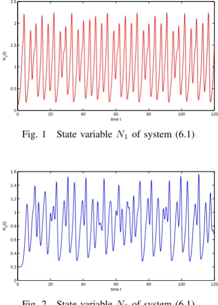
of Corollary 1 are satisfied. By Corollary 1, system (6.1) admits at least one positive almost periodic solution (see Figures 1-2). It is easy to verify that all the conditions of Theorems 2-3 are satisfied. By Theorems 2-3, system (6.1) is permanent and uniform asymptotical stability.

Remark 2. In system (6.1), corresponding to system (1.4)

and Corollary 3.3,ϕ1= √π₃,ϕ2=√π₂,βi,γi,σj andψare

arbitrary constants,i= 1,2,j = 1,2,3. So system (6.1) is with incommensurable periods. Through all the coefficients of system (6.1) are periodic functions, the positive periodic solutions of system (6.1) could not possibly exist. However, by Corollary 1, the positive almost periodic solutions of system (6.1) exactly exist.

IAENG International Journal of Applied Mathematics, 49:2, IJAM_49_2_03

(9)

0 20 40 60 80 100 120 0

0.5 1 1.5 2 2.5

time t

N1

(t)

Fig. 1 State variableN1 of system (6.1)

0 20 40 60 80 100 120

0 0.2 0.4 0.6 0.8 1 1.2 1.4 1.6

time t

N2

(t)

Example 3. Consider the following delayed almost periodic

predator-prey system:



            

            

˙

N1(t) = N1(t)

1−|sin √

2t|+|sin√3t|

2 N

2

1(t−0.8)

−₂_e10N1[1+(Nt)2 1(t)]

N2(t−0.8)

,

˙

N2(t) = N2(t)

− e−18

2+2e−18

−cos2( √

2t)+cos2(√3t)

2 N

2

2(t−0.8)

+ N12(t−0.8)

1+N2 1(t−0.8)

.

(6.2)

In system (6.2), |sin

√

2t|+|sin√3t|

2 and

cos2(√2t)+cos2(√3t)

2 are

almost periodic functions, which are not periodic functions. Similar to the argument as that in Example 2, by Theorem 1, it is easy to obtain that system (6.2) admits at least one positive almost periodic solution (see Figures 3-4).

0 20 40 60 80 100 120

0 0.5 1 1.5 2 2.5

time t

N1

(t)

0 20 40 60 80 100 120

0 0.5 1 1.5 2 2.5

time t

N2

(t)

VII. CONCLUSION

In this paper we have obtained the uniform permanence and existence of a positive almost periodic solution for a delayed predator-prey system with general functional re-sponse. The approach is based on the continuation theorem of coincidence degree theory and the comparison theorem. And Lemma 2 in Section 2 and Lemmas 2.3-2.4 in [22] are critical to study the permanence of the biological model. It is important to notice that the approach used in this paper can be extended to other types of biological model such as epidemic models, Lotka-Volterra systems and other similar models of first order.

VIII. ACKNOWLEDGEMENTS

This work is supported by the project of construction of first-class disciplines in Ningxia High School of China under Grant No. NXYLXK2017B11, Ningxia Normal University of China under Grant No. NXSFZDB1801 and Ningxia Natural Science Foundation under Grant No. 2018AAC03239.

REFERENCES

[1] D. Jana, S. Chakraborty, N. Bairagi, ”Stability, nonlinear oscillations and bifurcation in a delay-induced predator-prey system with harvest-ing”,Engineering Letters20:3, 238-246, 2012.

[2] L.L. Wang, P.L. Xie, ”Permanence and extinction of delayed stage-structured predator-prey system on time scales”, Engineering Letters

25:2, 147-151, 2017.

[3] S.B. Hsu, T.W. Hwang, Y. Kuang, ”Global analysis of the Michaelis-Menten type ratio-dependent predator-prey system”,J. Math. Biol.42: 489-506, 2011.

[4] M. Fan, K. Wang, ”Global existence of positive periodic solutions of periodic predator-prey system with infinite delays”,J. Math. Anal. Appl.

262: 1-11, 2001.

[5] S. Liu, E. Beretta, ”A stage-structured predator-prey model of Beddington-DeAngelis type”, SIAM J. Appl. Math. 66: 1101-1129, 2006.

[6] Z.Q. Zhang, X.W. Zheng, ”A periodic stage-structure mode”, Appl. Math. Lett.16: 1053-1061, 2003.

[7] L.L. Wang, W.T. Li, ”Existence and global stability of positive periodic solutions of a predator-prey system with delays”,Appl. Math. Comput.

146: 167-185, 2006.

[8] H.F. Huo, W.T. Li, ”Positive periodic solutions of a class of delay differential system with feedback control”,Appl. Math. Comput.148: 35-46, 2004.

[9] R. Xu, M.A.J. Chaplain, F.A. Davidson, ”Periodic solutions for a predator-prey model with Holling-type functional response and time delays”,Appl. Math. Comput.161: 637-654, 2005.

[10] H.L. Wang, ”Dispersal permanence of periodic predator-prey model with Ivlev-type functional response and impulsive effects”,Appl. Math. Model.34: 3713-3725, 2010.

[11] X. Ding, C. Lu, M. Liu, ”Periodic solutions for a semi-ratio-dependent predator-prey system with nonmonotonic functional response and time delay”,Nonlinear Anal.: RWA9: 762-775, 2008.

[12] C.J. Zhao, ”On a periodic predator-prey system with time delays”,J. Math. Anal. Appl.331: 978-985, 2007.

IAENG International Journal of Applied Mathematics, 49:2, IJAM_49_2_03

[image:9.595.320.535.58.188.2] [image:9.595.62.278.60.362.2] [image:9.595.64.279.642.778.2]

(10)

[13] G.R. Liu, J.R. Yan, ”Positive periodic solutions for neutral delay ratio-dependent predator-prey model with Holling type III functional response”,Appl. Math. Comput.218: 4341-4348, 2011.

[14] K. Wang, ”Existence and global asymptotic stability of positive periodic solution for a predator-prey system with mutual interference”,

Nonlinear Anal.: RWA10: 2774-2783, 2009.

[15] Y.L. Zhu, K. Wang, ”Existence and global attractivity of positive periodic solutions for a predator-prey model with modified Leslie-Gower Holling-type II schemes”,J. Math. Anal. Appl.384: 400-408, 2011.

[16] M.E. Gilpin, F.G. Ayala, ”Global models of growth and competition”,

Proc. Nat. Acad. Sci. USA70: 3590-3593, 1973.

[17] F.E. Smith, ”Population dynamics in Daphnia magna and a new model for population growth”,Ecology44: 651-663, 1963.

[18] C.Y. He, Almost Periodic Differential Equations, Higher Education Publishing House, Beijing, 1992 (Chinese).

[19] A.M. Fink,Almost Periodic Differential Equations, Springer, Berlin, 1974.

[20] R.E. Gaines, J.L. Mawhin,Coincidence Degree and Nonlinear Differ-ential Equations, Springer, Berlin, 1977.

[21] T.W. Zhang, ”Almost periodic oscillations in a generalized Mackey-Glass model of respiratory dynamics with several delays”, Int. J. Biomath.7: 1-22, 2014.

[22] X.L. Lin, Y.L. Jiang and X.Q. Wang, ”Existence of periodic solutions in predator-prey with Watt-type functional response and impulsive effects”,Nonlinear Anal.: TMA, 73, 1684-1697, 2010.