Defining Locality in Genetic Programming
to Predict Performance
Edgar Galv´an-L´opez, James McDermott, Michael O’Neill and Anthony Brabazon
Abstract— A key indicator of problem difficulty in evo-lutionary computation problems is the landscape’s locality, that is whether the genotype-phenotype mapping preserves neighbourhood. In genetic programming the genotype and phenotype are not distinct, but the locality of the genotype-fitness mapping is of interest. In this paper we extend the original standard quantitative definition of locality to cover the genotype-fitness case, considering three possible definitions. By relating the values given by these definitions with the results of evolutionary runs, we investigate which definition is the most useful as a predictor of performance.
I. INTRODUCTION
The concept of a fitness landscape [1] has dominated the way geneticists think about biological evolution and has been adopted within the Evolutionary Computation (EC) community. In simple terms, a fitness landscape can be seen as a plot where each point on the horizontal axis represents all the genes in an individual corresponding to that point. The fitness of that individual is plotted as the height against the vertical axis. Thus, a fitness landscape is a representation of a search space which may contain peaks, valleys, hills and plateaus.
How an algorithm explores and exploits such a landscape is a key element of evolutionary search. Rothlauf [2], [3] has described and analysed the importance of locality in perform-ing an effective evolutionary search of landscapes. Locality refers to how well neighboring genotypes correspond to neighboring phenotypes, and is useful as an indicator of problem difficulty. This research distinguished two forms of locality, low and high. A representation has high local-ity if all neighboring genotypes correspond to neighboring phenotypes, that is small genotypic changes result in small phenotypic changes. On the other hand, a representation has low locality if many neighboring genotypes do not correspond to neighboring phenotypes. It is demonstrated that a representation of high locality is necessary for efficient evolutionary search. In Section III we further explain the concept of locality.
In his original studies, Rothlauf used bitstrings to conduct his experiments [4] (and more recently he further explored the idea of locality using grammatical evolution at the chro-mosome level [5]). To our knowledge, there are few explicit studies on locality1 using the typical Genetic Programming
Edgar Galv´an-L´opez, James McDermott, Michael O’Neill and Anthony Brabazon are with the University College Dublin, Natural Computing Research & Applications Group, UCD CASL, 8 Belfield Office Park, Beaver Row, Clonskeagh, Dublin 4, email: edgar.galvan, james.mcdermott2, m.oneill,
1Initial preliminary results include [6].
(GP) [7], [8] representation (i.e., tree-like structures). For this purpose we will extend the definition of locality to GP, and due to the lack of distinction between genotype and phenotype, we will study the locality of the genotype-fitness mapping. The principle of strong causality states that for successful search, a small change in genotype should result in a small change in fitness [9]. The goal of this paper then is to shed some light on the type of locality present in GP and to clarify the correct extension of Rothlauf’s genotype-phenotype locality to the genotype-fitness case. We use three different mutation operators, three different genotypic dis-tance measures, and two problems with significantly different landscape features: the Artificial Ant Problem (a multimodal deceptive landscape) [10] and the Even-3-Parity Problem (a highly neutral landscape) [11].
This paper is organised as follows. In the next section, previous work on prediction of performance is summarised. In Section III locality in EC is presented. In Section IV, we describe how we study the locality of the genotype-fitness mapping in GP. In Section V, we present and discuss our findings. Finally, in Section VI we draw some conclusions.
II. RELATEDWORK
Landscapes and problem difficulty have been the subject of a good deal of research in EC in general and GP in particular. Several approaches to investigating problem difficulty have been proposed. In this section we mention some of them, including their pros and cons, which have inspired our work.
A. Fitness Distance Correlation
Jones [12], [13] proposed the fitness distance correlation
(fdc) to measure the difficulty of a problem on the basis of the relationship between fitness and distance. The idea behind
fdc was to consider fitness functions as heuristic functions and to interpret their results as indicators of the distance to the nearest optimum of the search space.fdcis an algebraic measure to express the degree to which the fitness function conveys information about distance to the searcher.
The definition of fdc is quite simple: given a set F = {f1, f2, ..., fn} of fitness values of n individuals and the
corresponding setD ={d1, d2, ..., dn} of distances of such
individuals from the nearest optimum, fdc is given by the following correlation coefficient:
f dc= CF D σFσD
,
where:
CF D= 1 n
n
i=1
(fi−f)(di−d)
is the covariance of F and D, and σF, σD, f and d are
the standard deviations and means ofF andD, respectively. Thenindividuals used to computefdcare obtained via some form of random sampling.
According to [13], [12] a problem can be classified in one of three classes, depending on the value of f dc:
1) misleading (f dc ≥ 0.15), in which fitness tends to
increase with the distance from the global optimum; 2) difficult (−0.15< f dc <0.15), for which there is no
correlation between fitness and distance; and
3) easy(f dc≤ −0.15), in which fitness increases as the
global optimum approaches.
The threshold interval [-0.15, 0.15] was empirically deter-mined by Jones. In [13], [12], Jones also proposed to use scatter plots (distance versus fitness) whenfdcdoes not give enough information about the hardness of a problem.
1) Comments on Fitness Distance Correlation: Al-tenberg [14] argued that predicting the hardness of a problem when using only fitness and distance in an EC system presents some difficulties. For instance, neither crossover nor mutation are taken into account whenfdcis calculated. Other works have also shown some weaknesses on fdc [15], [16]. As it can be seen from the previous examples, fdc presents some weakness to predict the hardness of a given problem. Both [17] and [18] construct examples which demonstrate that the fdc can be “blinded” by particular qualities of the search space, and that it can be misleading. There is, however, a vast amount of work where Jones’ approach has been successfully used in a wide variety of problems [19], [20], [21]. Of particular interest is the work by Vanneschi and colleagues [22], [17], [23], [24] which concentrated on the use of fdcin the context of GP.
B. Fitness Clouds and Negative Slope Coefficients
Later work by Vanneschi and colleagues attempted to address weaknesses of thefdc with new approaches.Fitness clouds are scatter plots relating fitness with distance to the optimum, as used in thefdc. Here, however, a more sophis-ticated approach to sampling the data (intended to model the real sampling behaviour of an evolutionary algorithm) and its analysis is used. The negative slope coefficient[25], [26] and the variantfitness-proportional negative slope coefficient
[27] allow estimation of problem difficulty without requiring knowledge of the global optimum, making an fdc-style approach practical on real-world problems for the first time.
C. Other Landscape Measures
Several other approaches to studying landscapes and prob-lem difficulty have also been proposed, generally in a non-GP context, including: other measures of landscape correlation [28], [29];epistasis, which measures the degree of interaction between genes and is a component ofdeception[18]; mono-tonicity, which is similar tofdcin that it measures how often fitness improves despite distance to the optimum increasing [18]; and distance distortion which relates overall distance in the genotype and phenotype spaces [4]. All of these
measures are to some extent related. However, Rothlauf’s
locality approach, again related to all of the ideas above, is of particular interest and so is treated separately in the next section.
III. LOCALITY
Understanding of how well neighbouring genotypes cor-respond to neighbouring phenotypes is a key element in understanding evolutionary search [4], [3]. In the abstract sense, a mapping has localityif neighbourhood is preserved under that mapping2. In EC this generally refers to the mapping from genotype to phenotype. This topic is a worthy of study because if neighbourhood is not preserved, then the algorithm’s attempts to exploit the information provided by an individual’s fitness will be misled when the individual’s neighbours turn out to be very different.
Rothlauf’s work on locality [4], [3], [31] has shed new light on several problems. Rothlauf gives a quantitative definition: “the localitydmof a representation can be defined
as
dm=
dg(x,y)=dgmin
|dp(x, y)−dpmin|
wheredp(x, y)is the phenotypic distance between the
pheno-typesxp andyp,dg(x, y)is the genotypic distance between
the corresponding genotypes, anddpminresp.dgminis the min-imum distance between two (neighboring) phenotypes, resp. genotypes” [4] [p. 77; notation changed slightly]. Locality is thus seen as a continuous property rather than a binary one. The point of this definition is that it provides a single quantity which gives an indication of the behaviour of the genotype-phenotype mapping and can be compared between different representations. Note that the quantity dm is a measure of
phenotypic divergence, so it is low for situations of high locality, and vice versa.
It can be stated that there are two types of locality: low and high locality. A representation is said to have the property of high locality if all neighboring genotypes correspond to neighboring phenotypes. On the other hand, a representation has low locality if some neighboring genotypes do not correspond to neighboring phenotypes. Rothlauf claims that a representation that has high locality will be more efficient at evolutionary search. If a representation has high locality then any search operator has the same effects in both the genotype and phenotype space. It is clear then that the difficulty of the problem remains unchanged compared to an encoding in which no genotype-phenotype map is required.
This, however, changes when a representation has low lo-cality. To explain how low locality affects evolution, Rothlauf considered three different categories, taken from the work presented in [12] and explained previously. These are:
• easy, in which fitness increases as the global optimum approaches,
2The termlocalityhas also been used in an unrelated context, to refer to
• difficult, for which there is no correlation between fitness and distance and,
• misleading, in which fitness tends to increase with the distance from the global optimum.
If a given problem lies in the first category (i.e., easy), a low-locality representation will change this situation by making it more difficult and now, the problem will lie in the second category. This is due to low locality randomising the search. This can be explained by the fact that representations with low locality lead to uncorrelated fitness landscapes, so it is difficult for heuristics to extract information.
If a problem lies in the second category, a low-locality representation does not change the difficulty of the problem. There are representations that can convert a problem from difficult (class two) to easy (class one). However, to construct such a representation typically requires an understanding of the landscape equivalent to solving the problem.
Finally, if the problem lies in the third category, a rep-resentation with low locality will transform it so that the problem will lie in the second category. That is, the problem is less difficult because the search has become more random. As can be seen, this is a mirror image of a problem lying in the first category and using a representation that has low locality.
Although Rothlauf does not provide a threshold value to distinguish high and low locality, nevertheless it is possible to make relative comparisons between representations.
Note in particular Rothlauf’s treatment of neutrality. When distinct (but neighbouring) genotypes map to identical pheno-types, a quantity (dmin) isaddedto the sum. This is the same
quantity that is added when neighbouring genotypes diverge slightly (for bitstring phenotypes with hamming distance). That is, neutrality is regarded as a deviation from good locality. Whether neutrality is beneficial in general is a complex question and some works have shed light on this issue [19], [20], [21], [32], [33], [34], but this issue deserves consideration as we will see.
We now consider the correct way to define the locality of the genotype-fitness mapping. Recall that locality, in general, is the property of preservation of neighbourhood under a mapping. Rothlauf assumes that a distance measure exists on both genotype and phenotype spaces, that for each there is a minimum distance, and that neighbourhood can be defined in terms of minimum distance. In standard GP, there are no phenotypes distinct from genotypes. It is common therefore to study instead the behaviour of the mapping from genotype to fitness [35], and we take this approach here. We will also regard two individuals to be neighbours in the genotype space if they are separated by a single mutation. That is, a mutation operator defines the neighbourhood of individuals at the genotype space, adhering to the Jones [12] principle that each operator induces its own landscape. We will also study very large spaces of GP-style trees, and therefore we must sample the space rather than enumerate it.
However, the most difficult issue in this context is how to define neighbourhood in the fitness space. There are three
possibilities:
• The most straightforward extension of Rothlauf’s def-inition might regard two individuals as neighbours if the difference of their fitness values is 1.3 This leads to the following definition which we call the f dmin = 1 definition of locality.
dm= N
i=1|f d(xi, m(xi))−f dmin|
N (1)
where f d(xi, m(xi)) = |f(xi) − f(m(xi))| is the
fitness distance between a randomly-sampled individual
xi and the mutated individualm(xi),f dmin= 1 is the
minimum fitness distance between two individuals, and
N is the sample size.
• However, the above definition treats a fitness-neutral mutation as being just as bad for locality as a mutation causing a fitness divergence of two fitness units (as-suming integer-valued fitness). It might be preferable to redefine the minimum distance in the fitness space as zero, giving the same locality definition as above but withf dmin= 0. This we termthef dmin= 0definition of locality.
• Finally, it might be better to treat only true divergence of fitness as indicating poor locality. Therefore we might say that fitness divergence occurs only when the fitness distance between the pair of individuals is 2 or greater: otherwise the individuals are regarded as neighbours in the fitness space. This leads to the following definition, which we will callthe conditional definition of locality).
dm= N
i=1:f d(xi,m(xi))≥2f d(xi, m(xi))
N (2)
wheref dmin= 1.
Since we have noa priorireason to decide which of these three is the best definition of genotype-fitness locality, we will decide the issue by relating the values produced by each with performance achieved on EC runs.
IV. EXPERIMENTALSETUP
For our analysis, we have used two well-known difficult problems for GP: the Artificial Ant Problem [7] (which has been shown to have multimodal deceptive features [10, Chapter 9]) and the Even-3-Parity problem (a problem that is difficult if no bias favorable is added in any part of the algorithm). To see and compare the locality present on these problems, we have decided to use two different function sets (see Table I for a description of them) for each of the problems used in this work. The idea here is that each function set will give a different locality and different performance.
The first problem, the Artificial Ant Problem [7, pp. 147– 155], consists of finding a program that can successfully navigate an artificial ant along a path of 89 pellets of food on a 32 x 32 toroidal grid. When the ant encounters a
3Notice that in this work we are using problems of discrete values and
0 1 2 3 4 5 6 7 8 0
0.1 0.2 0.3 0.4 0.5 0.6 0.7 0.8
Fitness distance
Frequency
Artificial Ant Problem (3 Functions)
Structural Mutation OnePoint Mutation Subtree Mutation
0 1 2 3 4 5 6 7 8
0 0.1 0.2 0.3 0.4 0.5 0.6 0.7 0.8
Fitness distance
Frequency
Artificial Ant Problem (4 Functions)
Structural Mutation OnePoint Mutation Subtree Mutation
0 1 2 3 4 5 6 7 8
0 0.1 0.2 0.3 0.4 0.5 0.6 0.7 0.8
Fitness distance
Frequency
Even−3−Parity Problem (3 Functions)
Structural Mutation OnePoint Mutation Subtree Mutation
0 1 2 3 4 5 6 7 8
0 0.1 0.2 0.3 0.4 0.5 0.6 0.7 0.8
Fitness distance
Frequency
Even−3−Parity Problem (4 Functions)
[image:4.595.58.556.57.468.2]OnePoint Mutation Subtree Mutation
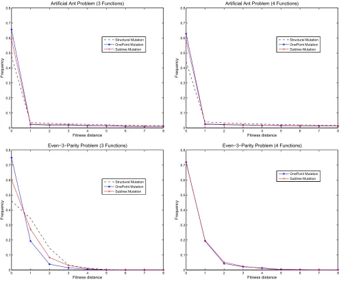
Fig. 1. Distribution of fitness distance values on the Artificial Ant Problem (top) and on the Even-3-Parity problem (bottom) using structural, one-point and subtree mutation, with standard and alternative function sets (left and right). For clarity we focus on the first 9 fitness distance values for the Artificial Ant Problem. Note also that structural mutation cannot be applied when using the 4-function set since all functions are of the same arity.
TABLE I
FUNCTION SETS USED ON THEARTIFICIALANT AND THEEVEN-3-PARITYPROBLEM.
Number of Artificial Ant Problem Even-3-Parity
functions
3 Functions FA3={IF, P ROG2, P ROG3} FE3={N OT, AN D, OR}
4 Functions FA3={IF, P ROG2, P ROG3, P ROG4} FE4={AN D, OR, N AN D, N OR}
food pellet, its (raw) fitness increases by one, to a maxi-mum of 89. The problem is in itself challenging for many reasons. The ant must eat all the food pellets (normally in 600 steps) scattered along a twisted track that has single, double and triple gaps along it. The terminal set used for this problem is T = {M ove, Right, Lef t}. The standard function set is FA3 = {IfFoodAhead, P rog2, P rog3} (see
[7] for a full description). In order to have an alternative encoding (with, as we will see, different performance and
locality characteristics), we now propose a second function set:FA4={IfFoodAhead, P rog2, P rog3, P rog4}. The only
difference is the addition of an extra sequencing function, Prog4, which runs each of its four subtree arguments in order. The second problem is the Boolean Even-3-Parity where the goal is to evolve a function that returns true if an even number of the inputs evaluate to true, and false otherwise. The maximum fitness for this problem is 8 (23). The terminal
T = {D0, D1, D2}. The standard function set is FE3 = {N OT, OR, AN D} and again, we propose a new function set for comparison: FE4 = {AN D, OR, N AN D, N OR}.
Each of the function sets is complete and sufficient to represent an optimal solution (indeed, any boolean function). Again our assumption, shown below to be correct, is that they will differ in performance and in locality characteristics.
For our studies we have considered the use of three different mutation operators:
• Subtree mutation replaces a randomly selected subtree with another randomly created subtree [7].
• One-Point mutation replaces a node (leaf or internal) in the individual by a new node chosen randomly among those of the same arity, taking the arity of a leaf as zero. In standard GP one-point mutation is generally applied with a per-node probability, but in our experiments, since we define genotypic neighbourhood in terms of single mutations, we will apply a single one-point mutation per mutation event.
• Structural mutation is composed of two complementary parts, inflate and deflate mutation. The former consists of inserting a terminal node beneath a function whose arity ais lower than the maximum arity defined in the function set and replacing the function by another of arity a+ 1; the latter consists of deleting a terminal
beneath a function whose arity is at least 1 and re-placing that function by another of arity a−1 [23]. Note that this mutation operator can only be applied when functions of the appropriate arity exist: in par-ticular, the alternative boolean function set (FE4 = {AN D, OR, N AN D, N OR}) contains functions all of arity 2, and so structural mutation will not be applicable. To have sufficient statistical data, we created 1,250,000 individuals for each of the three mutation operators described previously (in total 3,750,000 individuals). These samplings were created using traditional ramped half-and-half initialisa-tion method described in [7] using depths= [1,8]. By using
this method, we guarantee that we will use trees of different sizes and shapes, so no bias is imposed in our sampling.
For each data point in the sample data, we created an offspring via mutation, as in our locality definitions (Sec-tion III). In the following sec(Sec-tion we present and describe the results on locality using these mutations on the two problems using the two function sets and three mutation operators for each.
V. RESULTS
We begin by visually examining the distributions of fitness distances induced by the mutation operators. Figure 1 shows the frequency of each possible fitness distance (f d) between individuals, for the two problems and two function sets for each problem.
For the Artificial Ant Problem, fitness differences of up to 89 are possible, but larger values are rare and decrease roughly linearly, continuing the trend shown in Figure 1 (top). We have therefore omitted values above 8 to make
TABLE II
PARAMETERS USED TO CONDUCT OUR EXPERIMENTS.
Selection Tournament (size 7)
Initial Population Ramped half and half (depth 1 to 8) Population size 50, 100, 125, 200, 250, 500 Generations 500, 250, 200, 125, 100, 50
Runs 50
Mutations One Point, Subtree, Structural Mutation rate One single mutation per individual Termination Maximum number of generations
the important values easier to visualise. We can see that a high number of mutations are fitness-neutral (fitness distance = 0), regardless of the function set or mutation used. Using four function (FA4) produces slightly fewer fitness-neutral
mutations, with a proportional increase for larger fitness differences. We can also see that only a small proportion of individuals are fitness-neighbours (defined as f d = 1).
For larger fitness difference values (i.e., f d >1), it is very
difficult to see a difference between the 3- and 4-member function sets FA3 and FA4. As we will see, however, the
locality equations do distinguish between these cases. The Even-3-Parity Problem has 8 fitness cases; 9 possible fitness values, including 0; and 9 possible fitness distances. The frequency of occurrence of each fitness distance is shown in Figure 1 (bottom). The number of neutral mutations (f d = 0) is again much larger compared to
non-fitness-neutral mutations (f d > 0), regardless of the function set
used. For the standard function set (FE3), it seems that
one-point mutation produces the greatest number of fitness-neutral mutations (i.e., f d = 0), followed by subtree and
structural mutation. Structural mutation seems to produce the greatest number of fitness neighbours (i.e., f d= 1). When using FE4, the situation is less clear and again, one really
needs to take a look at the results on locality by using the locality equations, discussed next.
A. Evolutionary Runs
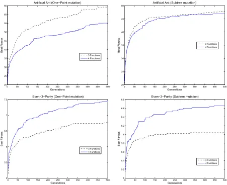
To see if the prediction made by locality (Equation 1) is correct, we performed actual runs for each of the problems presented in Section IV and the two instances on each on them (i.e., two different function sets). For this purpose, we used a mutation-GP system (using each of the three mutation operators in separate runs). According to the one-operator, one-landscape principle [12], and since we define locality using mutation only, crossover was not used. This methodology is standard [5]. To obtain meaningful results, we performed 50 independent runs, using different combina-tions of population sizes and generacombina-tions. Runs were stopped when the maximum number of generations was reached. The rest of the parameters are shown in Table II. The best fitness per generation, averaged over 50 runs, is shown in Figure 2.
B. Comparing alternative encodings
0 50 100 150 200 250 300 350 400 450 500 20
25 30 35 40 45 50 55 60 65
Generations
Best Fitness
Artificial Ant (One−Point mutation)
3 Functions 4 Functions
0 50 100 150 200 250 300 350 400 450 500
20 25 30 35 40 45 50
Generations
Best Fitness
Artificial Ant (Subtree mutation)
3 Functions 4 Functions
0 50 100 150 200 250 300 350 400 450 500
5 5.5 6 6.5 7 7.5
Generations
Best Fitness
Even−3−Parity (One−Point mutation)
3 Functions 4 Functions
0 50 100 150 200 250 300 350 400 450 500
5 5.2 5.4 5.6 5.8 6 6.2 6.4 6.6 6.8
Generations
Best Fitness
Even−3−Parity (Subtree mutation)
[image:6.595.75.526.56.424.2]3 Functions 4 Functions
Fig. 2. Best fitness for the Artificial Ant Problem (top) and the Even-3-Parity problem (bottom) and using two mutation operators: one-point (left) and subtree mutation (right).
In Tables III and IV, we show the locality of the two prob-lems (Artificial Ant and Even-3-Parity) and their instances (i.e., two different function sets shown in Table I) and three mutation operators. For the Artificial Ant Problem (Table III), we can see that the function set FA3 has better properties
of locality (i.e., lower number) compared to FA4. That is,
the typical function set used for this problem and using any of the mutations used in this work (one-point, subtree and structural) is predicted to be better. For the Even-3-Parity Problem, the best properties of locality are when usingFE4
(i.e.,AN D, OR, N AN D, N OR).
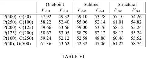
We now relate these predictions to performance (e.g., aver-age of best fitness per run or finding a solution). For this, we used six different values for the population size as well as for numbers of generations, giving a total of 25,000 individuals in every case. Let us start our analysis by looking at the results found on the Artificial Ant Problem (see Table V). According to the results on locality shown in Table III, we should expect to see a better performance (in terms of the average of the best fitnesses out of 50 independent runs) when using FA3 and using any of the three mutation
operators. In fact, we can see that the best performance is achieved when using FA3. This was correctly predicted
using all three definitions of locality: in all combinations of population size and number of generations, they gave a better locality value forFA3 (i.e.,IF, P ROG2, P ROG3). In fact,
this is consistent with the best fitness per generation on the 50 independent runs using 50 individuals and 500 generations4 (see top of Figure 2).
For our second problem (Even-3-Parity), the prediction obtained using the f d= 1 definition of locality was again correct, but the other definitions did not predict the differing performance (see Table IV). In this case, we can see that there are better properties of locality when using FE4 (i.e., AN D, OR, N AN D, N OR) on the one-point and subtree mutation (structural mutation being inapplicable with this function set). This is, in fact, the case for all the combinations we tested on this problem (see Table VI, where the best per-formance (measured in terms of finding the global optimum)
4Due to space constraints we show only these combinations of values for
TABLE III
LOCALITY ON THEARTIFICIALANTPROBLEM USING TWO FUNCTION
SETS(FA3={IF, P ROG2, P ROG3}AND
FA4={IF, P ROG2, P ROG3, P ROG4}),THREE MUTATIONS,AND THREE LOCALITY DEFINITIONS.
f dmin= 0 f dmin= 1 f dmin≤1
FA3 FA4 FA3 FA4 FA3 FA4
[image:7.595.313.556.131.229.2]One Point 1.8790 2.0896 2.1467 2.2628 1.5128 1.6764 Subtree 2.1653 2.2804 2.3199 2.3708 1.7426 1.8256 Structural 2.1771 2.4162 2.3197 2.4124 1.7484 1.9143
TABLE IV
LOCALITY ON THEEVEN-3-PARITYPROBLEM USING TWO FUNCTION
SETS(FE3={AND, OR, NOT}AND
FE4={AND, OR, NAND, NOR}),THREE MUTATIONS,AND THREE LOCALITY DEFINITIONS. RECALL THAT STRUCTURAL MUTATION IS
INAPPLICABLE WITHFE4.
f dmin= 0 f dmin= 1 f dmin≤1
FE3 FE4 FE3 FE4 FE3 FE4
One Point 0.0968 0.1435 0.9196 0.8904 0.0082 0.0169 Subtree 0.1368 0.1368 0.8780 0.8760 0.0064 0.0069 Structural 0.1769 NA 0.8740 NA 0.0254 NA
is seen when using FE4. Again, as for the Artificial Ant
Problem, this is consistent with the best fitness per generation on the runs performed to corroborate the prediction obtained with locality (see bottom of Figure 2 where population size = 50 and generations = 500).
C. Comparing alternative mutation operators
We next compare the locality properties of the three mutation operators, comparing the results given by the three locality definitions with the performance in actual GP runs. Comparing Tables III and V, we see that on the Artificial Ant problem, locality is best for the one-point operator according to all three definitions. However, performance was mixed: the one-point operator sometimes performed better in evolutionary runs than the other operators, sometimes worse (using either encoding). Thus none of the three locality definitions predicted performance correctly here. There was little to choose between subtree and structural mutation in this case.
On the Even-3 Parity problem, the one-point mutation operator now has worse locality, according to thef dmin= 1
and the conditional definitions of locality (Figure IV). These predictions are seen to be correct when we look at perfor-mance (Figure VI). The f dmin = 0 definition of locality
gives mixed messages concerning performance (Figure IV).
VI. CONCLUSIONS
Rothlauf [4] described and analysed the importance of locality in performing an effective evolutionary search of landscapes. According to Rothlauf, a representation that has high locality is necessary for an efficient evolutionary search. In this work, we have extended Rothlauf’s quantitative definition of phenotype locality to the genotype-fitness mapping, considering the issues of genotype-fitness
neighbour-TABLE V
AVERAGE OF THE BEST FITNESSES OUT OF50INDEPENDENT RUNS OF A MUTATION-BASEDGPON THEARTIFICIALANTPROBLEM USING
THREE TYPES OF MUTATIONS: ONEPOINT, SUBTREE ANDSTRUCTURAL MUTATION.FA3={IF, P ROG2, P ROG3}AND
FA4={IF, P ROG2, P ROG3, P ROG4}.
OnePoint Subtree Structural FA3 FA4 FA3 FA4 FA3 FA4
P(500), G(50) 57.92 49.32 59.10 53.78 57.10 54.26 P(250), G(100) 58.22 52.40 55.06 52.14 61.01 54.82 P(200), G(125) 59.66 53.66 59.00 53.76 58.12 55.24 P(125), G(200) 58.67 53.05 58.79 52.12 58.12 55.24 P(100), G(250) 59.24 52.12 52.58 48.86 60.46 55.52 P(50), G(500) 61.36 53.62 52.32 47.06 61.22 58.74
TABLE VI
PERFORMANCE(MEASURED IN TERMS OF FINDING THE GLOBAL
OPTIMUM)OF AMUTATION-BASEDGPON THEEVEN-3-PARITY PROBLEM USING THREE TYPES OF MUTATIONS: ONEPOINT, SUBTREE
ANDSTRUCTURALMUTATION.FE3={NOT, AND, OR}AND FE4={NAND, NOR, AND, OR}.
OnePoint Subtree Structural FE3 FE4 FE3 FE4 FE3 FE4
P(500), G(50) 4% 18% 0% 4% - NA
P(250), G(100) 4% 18% 10% 16% - NA
P(200), G(125) 2% 28% 6% 14% - NA
P(125), G(200) 6% 32% 4% 12% - NA
P(100), G(250) 6% 28% 2% 16% - NA
P(50), G(500) 6% 46% 6% 28% - NA
hood and neutrality in particular. For this purpose, we have used two problems with significantly different landscape features: a multimodal deceptive landscape and a highly neutral landscape (both believed to be common in many real-world problems). We have used two instances for each of these problems and analysed the locality present on them by defining neighbourhood in the fitness space in three different ways: when the fitness distance is 0 (f d= 0), when it is 1
(f d= 1) and a combination of these (i.e., whenf d <2, the
individuals are treated as neighbours).
We have seen that the correct prediction was obtained more often when neighbourhood was defined with f d= 1,
which corresponds to the definition given by Rothlauf in his genotype-phenotype mapping studies using bitstrings [4]. To corroborate this finding, we performed independent runs and used different combinations of population sizes and generations (i.e., six in total). In all of them, this definition of locality correctly predicted the differing performance of the two function sets.
of the mutation operators.
Nevertheless, we can conclude that performance is best predicted by a genotype-fitness locality definition which takes individuals as fitness neighbours if they differ by 1 fitness unit, and which treats fitness-neutrality as detrimental to locality.
ACKNOWLEDGMENTS
This research is based upon works supported by Science Foundation Ireland under Grant No. 08/IN.1/I1868 and by the Irish Research Council for Science, Engineering and Technology under the Empower scheme.
REFERENCES
[1] S. Wright, “The Roles of Mutation, Inbreeding, Crossbreeding and Selection in Evolution,” in Proceedings of the Sixth International Congress on Genetics, D. F. Jones, Ed., vol. 1, 1932, pp. 356–366. [2] F. Rothlauf and D. Goldberg, “Redundant Representations in
Evolu-tionary Algorithms,” Evolutionary Computation, vol. 11, no. 4, pp. 381–415, 2003.
[3] F. Rothlauf and M. Oetzel, “On the locality of grammatical evolution,” in Proceedings of the 9th European Conference on Genetic Programming, ser. Lecture Notes in Computer Science, P. Collet, M. Tomassini, M. Ebner, S. Gustafson, and A. Ek´art, Eds., vol. 3905. Budapest, Hungary: Springer, 10 - 12 Apr. 2006, pp. 320–330. [Online]. Available: http://link.springer.de/link/service/series/0558/papers/3905/39050320.pdf [4] F. Rothlauf,Representations for Genetic and Evolutionary Algorithms,
2nd ed. Physica-Verlag, 2006.
[5] F. Rothlauf and M. Oetzel, “On the Locality of Grammatical Evolu-tion,” inEuroGP, ser. Lecture Notes in Computer Science, P. Collet, M. Tomassini, M. Ebner, S. Gustafson, and A. Ekart, Eds., vol. 3905. Springer, 2006, pp. 320–330.
[6] E. Galvan-Lopez, M. O’Neill, and A. Brabazon, “Towards Understand-ing the Effects of Locality in GP,”Mexican International Conference on Artificial Intelligence, pp. 9–14, 2009.
[7] J. R. Koza,Genetic Programming: On the Programming of Computers by Means of Natural Selection. Cambridge, Massachusetts: The MIT Press, 1992.
[8] R. Poli, W. B. Langdon, and N. F. McPhee, A field guide to genetic programming. Published via http://lulu.com and freely available at http://www.gp-field-guide.org.uk, 2008, (With contributions by J. R. Koza). [Online]. Available: http://www.gp-field-guide.org.uk
[9] H. Beyer and H. Schwefel, “Evolution strategies–A comprehensive introduction,”Natural Computing, vol. 1, no. 1, pp. 3–52, 2002. [10] W. B. Langdon and R. Poli, Foundations of Genetic Programming.
Berlin: Springer, 2002.
[11] M. Collins, “Finding needles in haystacks is harder with neutrality,” inGECCO ’05: Proceedings of the 2005 conference on Genetic and evolutionary computation. New York, NY, USA: ACM, 2005, pp. 1613–1618.
[12] T. Jones, “Evolutionary algorithms, fitness landscapes and search,” Ph.D. dissertation, University of New Mexico, Albuquerque, 1995. [13] T. Jones and S. Forrest, “Fitness Distance Correlation as a Measure
of Problem Difficulty for Genetic Algorithms,” inProceedings of the 6th International Conference on Genetic Algorithms, L. J. Eshelman, Ed. San Francisco, CA, USA: Morgan Kaufmann Publishers, 1995, pp. 184–192.
[14] L. Altenberg, “Fitness Distance Correlation Analysis: An Instructive Counterexample,” inProceedings of the Seventh International Confer-ence on Genetic Algorithms, T. Back, Ed. San Francisco, CA, USA: Morgan Kaufmann, 1997, pp. 57–64.
[15] R. J. Quick, V. J. Rayward-Smith, and G. D. Smith, “Fitness Distance Correlation and Ridge Functions,” inProceedings of the 5th Interna-tional Conference on Parallel Problem Solving from Nature. London, UK: Springer-Verlag, 1998, pp. 77–86.
[16] M. Clergue and P. Collard, “GA-Hard Functions Built by Combination of Trap Functions,” inCEC 2002: Proceedings of the 2002 Congress on Evolutionary Computation, D. B. Fogel, M. A. El-Sharkawi, X. Yao, G. Greenwood, H. Iba, P. Marrow, and M. Schackleton, Eds. IEEE Press, 2002, pp. 249–254.
[17] M. Tomassini, L. Vanneschi, P. Collard, and M. Clergue, “A study of fitness distance correlation as a difficulty measure in genetic programming,”Evolutionary Computation, vol. 13, no. 2, pp. 213– 239, 2005.
[18] B. Naudts and L. Kallel, “A comparison of predictive measures of problem difficulty in evolutionary algorithms,”IEEE Transactions on Evolutionary Computation, vol. 4, no. 1, pp. 1–15, April 2000. [19] E. Galv´an-L´opez and R. Poli, “Some Steps Towards Understanding
How Neutrality Affects Evolutionary Search,” in Parallel Problem Solving from Nature (PPSN IX). 9th International Conference, ser. LNCS, T. P. Runarsson, H.-G. Beyer, E. Burke, J. J. Merelo-Guerv´os, L. D. Whitley, and X. Yao, Eds., vol. 4193. Reykjavik, Iceland: Springer-Verlag, 9-13 Sep. 2006, pp. 778–787.
[20] R. Poli and E. Galv´an-L´opez, “On The Effects of Bit-Wise Neutrality on Fitness Distance Correlation, Phenotypic Mutation Rates and Prob-lem Hardness,” inFoundations of Genetic Algorithms IX, ser. Lecture Notes in Computer Science, C. R. Stephens, M. Toussaint, D. Whitley, and P. Stadler, Eds. Mexico city, Mexico: Springer-Verlag, 8-11 Jan. 2007, pp. 138–164.
[21] E. Galv´an-L´opez, S. Dignum, and R. Poli, “The Effects of Constant Neutrality on Performance and Problem Hardness in GP,” inEuroGP 2008 - 11th European Conference on Genetic Programming, ser. LNCS, M. ONeill, L. Vanneschi, S. Gustafson, A. I. E. Alcazar, I. D. Falco, A. D. Cioppa, and E. Tarantino, Eds., vol. 4971. Napoli, Italy: Springer, 26–28 Mar. 2008, pp. 312–324.
[22] M. Tomassini, L. Vanneschi, P. Collard, and M. Clergue, “A Study of Fitness Distance Correlation as a Difficulty Measure in Genetic Programming,”Evolutionary Computation, vol. 13, no. 2, pp. 213– 239, Summer 2005.
[23] L. Vanneschi, “Theory and practice for efficient genetic program-ming,” Ph.D. dissertation, Faculty of Science, University of Lausanne, Switzerland, 2004.
[24] L. Vanneschi, M. Tomassini, P. Collard, and M. Clergue, “Fitness distance correlation in structural mutation genetic programming,” in EuroGP, ser. Lecture notes in computer science. Springer, 2003, pp. 455–464.
[25] L. Vanneschi, M. Clergue, P. Collard, M. Tomassini, and S. Verel, “Fitness clouds and problem hardness in genetic programming,” in EuroGP, ser. LNCS. Springer, 2004, pp. 690–701.
[26] L. Vanneschi, M. Tomassini, P. Collard, S. Verel, Y. Pirola, and G. Mauri, “A comprehensive view of fitness landscapes with neutrality and fitness clouds,” inProceedings of EuroGP 2007, ser. LNCS, vol. 4445. Springer, 2007, pp. 241–250.
[27] R. Poli and L. Vanneschi, “Fitness-proportional negative slope coef-ficient as a hardness measure for genetic algorithms,” inProceedings of GECCO ’07, London, UK, 2007, pp. 1335–1342.
[28] E. Weinberger, “Correlated and uncorrelated fitness landscapes and how to tell the difference,”Biological Cybernetics, vol. 63, no. 5, pp. 325–336, 1990.
[29] W. Hordijk, “A measure of landscape,” Evolutionary Computation, vol. 4, no. 4, pp. 335–360, 1996.
[30] P. D’haeseleer and J. Bluming, “Effects of locality in individual and population evolution,” inAdvances in Genetic Programming, K. E. Kinnear, Ed. MIT Press, 1994, pp. 177–198.
[31] F. Rothlauf, “On the bias and performance of the edge-set encoding,” IEEE transactions on evolutionary computation, vol. 13, no. 3, pp. 486–499, June 2009.
[32] E. Galv´an-L´opez, “An Analysis of the Effects of Neutrality on Problem Hardness for Evolutionary Algorithms,” Ph.D. dissertation, School of Computer Science and Electronic Engineering, University of Essex, United Kingdom, 2009.
[33] P. K. Lehre and P. C. Haddow, “Phenotypic Complexity and Local Variations in Neutral Degree,”BioSystems, vol. 87, no. 2-3, pp. 233– 42, 2006.
[34] M. Toussaint and C. Igel, “Neutrality: A necessity for self-adaptation,” inProceedings of the IEEE Congress on Evolutionary Computation (CEC 2002), 2002, pp. 1354–1359.