Mathematical Modeling of Complex Fluids

(1)

The University of W¨urzburg Department of Mathematics

Mathematical Modeling of

Complex Fluids

Master’s Thesis

submitted by

Johannes Forster

Matr.-Nr. 1596004

in

March 2013

Advisor/reviewer: Prof. Dr. Anja Schl¨omerkemper Department of Mathematics University of W¨urzburg

Second reviewer: Prof. Dr. Chun Liu

(2)

(3)

List of Figures

1.1 States of matter changing with temperature . . . 3

2.1 Deformation Mapping between Reference Configuration ΩX 0 and

Deformed Configuration Ωx

t . . . 7

3.1 Mass attached to a Hookean spring . . . 15 3.2 Near initial data vs. near equilibrium dynamics . . . 21

(6)

(7)

Zusammenfassung

Die vorliegende Masterarbeit besch¨aftigt sich mit der mathematischen Model-lierung komplexer Fl¨ussigkeiten.

Nach einer Einführung in das Thema der komplexen Flüssigkeiten werden grundle-gende mechanische Prinzipien im zweiten Kapitel vorgestellt. Im Anschluss steht eine Einführung in die Modellierung mit Hilfe von Energien und eines varia-tionellen Ansatzes.

Dieser wird im vierten Kapitel auf konkrete Beispiele komplexer Flüssigkeiten angewendet. Dabei werden zunächst viskoelastische Materialien (z.B. Muskel-masse) angeführt und ein Modell für solche beschrieben, bei dem Eigenschaften von Festkörpern und Flüssigkeiten miteinander kombiniert werden.

Anschließend untersuchen wir den Ursprung solcher Eigenschaften und die Aus-wirkungen von bestimmten Molekülstrukturen auf das Verhalten der umgeben-den Flüssigkeit. Dabei betrachten wir zunächst ein Mehrskalen-Modell für Poly-merflüssigkeiten und damit eine Kopplung mikroskopischer und makroskopischer Größen. In einem dritten Beispiel beschäftigen wir uns dann mit einem Model für nematische Flüssigkristalle, die in technischen Bereichen, wie beispielsweise der Displaytechnik, Anwendung finden.

Geschlossen wird mit einem Ausblick auf weitere Anwendungsgebiete und mathe-matische Probleme.

(8)

(9)

1 Introduction

This thesis gives an overview over mathematical modeling of complex fluids with the discussion of underlying mechanical principles, the introduction of the ener-getic variational framework, and examples and applications.

The purpose is to present a formal energetic variational treatment of energies corresponding to the models of physical phenomena and to derive PDEs for the complex fluid systems.

The advantages of this approach over force-based modeling are, e.g., that for complex systems energy terms can be established in a relatively easy way, that force components within a system are not counted twice, and that this approach can naturally combine effects on different scales.

We follow a lecture of Professor Dr. Chun Liu from Penn State University, USA, on complex fluids which he gave at the University of W¨urzburg during his Gio-vanni Prodi professorship in summer 2012. We elaborate on this lecture and con-sider also parts of his work and publications, and substantially extend the lecture by own calculations and arguments (for papers including an overview over the energetic variational treatment see [HKL10], [Liu11] and references therein).

It is, of course, vital to understand what the term “complex fluids” is about, and what are, in contrast, “simple fluids”. When we talk about fluids we think of a certain state of matter. Usually, from our daily experience, everyone knows three states of matter. These are, in particular, the solid, the liquid, and the gas phase. In order to illustrate the three phases in a certain way, we come up with a simple line which stands for an increase of temperature in the direction of the arrow: Figure 1.1 shows what we have learned from our day to day life: If one

temperature

solid liquid gas

Figure 1.1: States of matter changing with temperature

takes, for example, a pot of water and heats it up, the water becomes steam, i.e., liquid becomes gas.

(10)

First, we need to consider what a (simple) state of matter is actually about. For this, we have a closer look at the materials, that means we look at the particles inside the material. If one takes a rigid piece of iron, a piece of ice or a grain of salt and studies the structure with the help of a microscope, it can be observed that the atoms are quite close together and form certain lattice structures. In the gas phase, however, the atoms have greater distances between each other and are free to move around. The atoms that form a liquid phase are somehow in between: They are closer together but do not form rigid lattices, so they can move quite freely around, i.e., the degree of freedom in motion is higher than within rigid solid lattices but lower than within gas phases.

Next we specify in more detail what is meant by “degree of freedom to move” within the phases. Here we talk aboutorder and interactions.

In terms of order we can distinguish between different sorts: Orientational and

positional order.

In the lattice structures of solid materials – we stick to the example of water, ice and steam for the moment – there is a high degree of positional order: The atoms are not free to move within the lattice which is due to strong interactions among the atoms. The atoms only vibrate on their fixed position within the structure. If we let the temperature increase, the vibrations of the atoms also increase and the interactions are “weakened”, thus ice becomes water. In this phase, there is also no positional order compared to the rigid lattice.

Letting the temperature increase even more, liquid water reaches the gas phase, where interactions and order are even lower.

A material which exhibits orientational order is called liquid crystalline material. A basic yet interesting material of this kind are nematic liquid crystals: It is like a bunch of rod shaped molecules which are free to move but tend to align in one common direction. Liquid crystals are widely seen in technical applications, such as displays or self-shading windows. The nematics, e.g., give name to the display technology “TN” which stands for “twisted nematic”. In fact, liquid crystals are an example for complex fluids: They can flow like a fluid but exhibit certain order or microstructures. We discuss liquid crystals later in Section 4.3.

Complex fluids can exhibit fluid properties (flow) as well as properties usually found in solid materials (order/structure). They form intermediate phases be-tween solids and fluids. Further examples are gels or volcanic lava: They flow but if one looks closer, certain solid structures can be found. These materials are called viscoelastic materials. Certain examples are discussed in Section 4.1.

The theory of complex fluids has also applications in biological and biochemical settings. Ionic solutions that run through our body are complex fluids, so the models can be used to understand chemical processes within our body or special organs.

(11)

notation we use for the forthcoming analysis as well as the setting we consider are defined there. This chapter also deals with several mechanical properties of matter.

Chapter 3 introduces the Energetic Variational Framework for the analysis of mechanical systems, kinematics and transport theory, and principles for Hamil-tonian and dissipative systems. We also give basic examples of simple solid and fluid systems and discuss what characterizes solid and fluid materials.

Models for complex fluids are then discussed in Chapter 4 with the use of formal energetic variational treatments. The first topic is a model for incompressible viscoelasticity to combine solid and fluid properties. We continue with a model for micro-macro-interactions in polymeric fluids and consider the coupling of microscopic and macroscopic variables. Afterwards we discuss (nematic) liquid crystalline material. Both the polymeric fluids and the nematics are considered in order to study the effect of embedded structures onto fluid flow properties. This chapter in particular contains elaborate calculations to derive the systems of partial differential equations from the energy laws of the different models. These calculations were left out for brevity in publications and the lecture.

(12)

(13)

2 Basic Mechanics

In this chapter we present the general setting we consider when studying complex fluids (c.f. [HKL10]). Moreover, we define several objects that help us to model, understand, and study these materials.

2.1 Coordinate Systems and Deformation

First, we define the deformation and talk about the different coordinate systems.

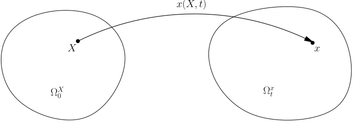
x(X, t)

Ωx t

ΩX

0

[image:13.595.133.489.302.425.2]

x X

Figure 2.1: Deformation Mapping between Reference Configuration ΩX

0 and De-formed Configuration Ωx

t

Definition 1. Let ΩX

0 , Ωxt ⊂Rn, n∈ N, be domains with smooth boundaries,

t∈R+

0 be time and letu= (u1, . . . , un) be a smooth vector field inRn depending

smoothly on time t. The deformation or flow map x(X, t) : ΩX

0 →Ωxt is defined

as a solution map of (_d

dtx(X, t) =u(x(X, t), t), t >0,

x(X,0) =X, (2.1)

where X= (X1, . . . , Xn)∈ΩX₀ andx= (x1, . . . , xn)∈Ωxt.

The coordinate system X is called the Lagrangian coordinate system and refers toΩX

0 which we call the reference configuration; the coordinate systemx is called

the Eulerian coordinate system and refers toΩxt which we call the deformed

con-figuration.

In other words, we start from a domain ΩX

0 , the reference configuration which

(14)

superscripts x and X just indicate the different coordinate systems. Later we consider integrals over the reference or deformed configuration. Then we also use x and X as integration variables.

The special term flow map is due to the dependency on two variables: If t is fixed, X 7→ x(X, t) maps the reference configuration ΩX

0 onto the deformed

configuration Ωx_t. We assume that this map is bijective since we map each particle in the reference configuration to its new position in the deformed configuration, this should be one-to-one and onto.

On the other hand, if X is fixed, i.e., we look at one special point or particle in the reference configuration, the map t 7→ x(X, t) denotes the changing position or the flow or trajectory of this particle over time.

These two ways of interpreting the deformation x(X, t) lead to the term flow map.

The vector fielduis the velocity, i.e., the derivative of the flow map with respect to time. The flow map is actually defined using the velocity vector field.

The Lagrangian coordinate system is usually used to describe the elastic behavior of solid materials where one looks at each particle X. However, the Eulerian coordinate system is used to model fluid materials where one looks at special positions x instead of single particles. Equation (2.1) links the two coordinate systems: Both sides describe the velocity of a particle labeled withX at position x and timet.

In the following we always assume that the flow map is smooth in both time and spatial variables, so all the calculations are well-defined. In particular, partial derivatives can be interchanged.

2.2 Deformation Gradient

In this section we take a look at the derivative of the flow map with respect to X and the properties of this important entity.

Definition 2. Let Fe be the Jacobian matrix of the mapX 7→x(X, t) defined by e

F(X, t) := ∂x(X, t)

∂X :=∇Xx(X, t) (2.2)

=

∂xi ∂Xj

1≤i,j≤n

=

  

∂x1

∂X1 · · · ∂x 1 ∂Xn ..

. ...

∂xn

∂X1 · · · ∂xn

∂Xn   .

e

F is called the deformation gradient.

(15)

The deformation gradient, by definition, carries the information about how the configuration is deformed with respect to the reference configuration. That means,Fe carries all the information about structures and patterns.

We assume that detF >e 0, so that the deformation gradient is an invertible matrix.

The following proposition gives an important result for the deformation gradient. We use it as a natural kinematic equation if the deformation gradient is involved in the model of a physical system. At first, we do apush forward forFe, i.e., we express the deformation gradient by the Eulerian coordinate system. Therefore, set

e

F(X, t) =F(x(X, t), t).

Proposition 4. F satisfies the equation

∂F

∂t +u· ∇xF =∇xu·F. (2.3)

Proof. By the chain rule, we obtain from the push forward

d

dtF(x(X, t), t) = ∂

∂tF(x(X, t), t) +u(x(X, t), t)· ∇xF(x(X, t), t). Furthermore, by using Definition 2 and the chain rule, we get

d

dtF(X, t) =e d dt

∂xi(X, t) ∂Xj

1≤i,j≤n

=

∂xi_t(X, t) ∂Xj

1≤i,j≤n

=

∂ui_{(x(X, t), t)}

∂Xj

1≤i,j≤n

=

n

X

k=1

∂ui_{(x(X, t), t)}

∂xk

∂xk_{(X, t)}

∂Xj

!

1≤i,j≤n

=∇xu(x(X, t), t)·Fe(X, t).

SinceF is defined byFe(X, t) =F(x(X, t), t), both equations are equal. Thus

∂

∂tF(x(X, t), t) +u(x(X, t), t)· ∇xF(x(X, t), t) =∇xu(x(X, t), t)·Fe(X, t), and with the push forward applied once again, we obtain

∂

∂tF(x(X, t), t) +u(x(X, t), t)· ∇xF(x(X, t), t) =∇xu(x(X, t), t)·F(x(X, t), t), which can be written in the Eulerian coordinate system as

∂

∂tF(x, t) +u(x, t)· ∇xF(x, t) =∇xu(x, t)·F(x, t). This concludes the proof.

(16)

Definition 5. Let M : Rn _→ Rn×n _{be a differentiable matrix field. The}

diver-gence of M, denoted by ∇ ·M, is defined by

(∇ ·M)i = n

X

j=1

∂

∂xjMij =∇jMij

for i = 1, . . . , n. In the second equation the Einstein summation convention is applied with the simplified notation ∇j := _∂x∂j.

By definition, the divergence of a matrix field is a vector field.

2.3 Incompressibility

In this section we turn to a very important property of materials. From a phys-ical point of view, incompressible flows are flows where the material density is constant in an infinitesimal volume element which moves along with the velocity of the fluid. We now give a mathematical definition.

Definition 6. Let x(X, t) be the deformation of a material. The material is said to be incompressible if detFe ≡1.

The formulation above is in the Lagrangian coordinate system, but by using the push forward Fe(X, t) = F(x(X, t), t) the same equation holds for F in the

Eulerian coordinate system.

However, there is another characterization of incompressibility in the Eulerian coordinate system, given by the following proposition.

Proposition 7. Let x(X, t) be the deformation of a material, Fe(X, t) the defor-mation gradient and u(x(X, t), t) the velocity. It holds

detFe≡1 ∀X∈ΩX₀ , t≥0 =⇒ ∇x·u= 0 ∀X∈ΩX0 , t≥0.

The converse is true if the initial data detFe(X,0) = 1 is given.

To be able to prove the proposition, we need two lemmas first.

Lemma 8. The inverse of the deformation gradient is Fe−1 = ∂X_∂x.

Proof. Since the flow map is assumed to be smooth, the bijective map X 7→

(17)

Lemma 9. Let A: R+

0 → GL(n,R) ⊂Rn×n be a time dependent differentiable

field of invertible matrices and letdet :Rn×n→Rbe the determinant. Then the derivative of t7→detA(t) with respect to timet is given by

d

dtdetA(t) = (detA) tr

A−1 d dtA

.

Proof. The derivative of the determinant detA with respect to the argument A (for a calculation see Appendix A.3) is

∂(detA) ∂A =A

−T _det_A.

Now, since detA(t) = det◦A(t), whereA:R+

0 →Rn×n and det :Rn×n→R, we

use the chain rule from Appendix A.2 and the product defined in Appendix A.1. We obtain

d

dtdetA(t) =

∂(detA) ∂A :

d dtA

= (detA)A−T :

d dtA

= (detA) tr

A−1 d dtA

.

This concludes the proof.

Now we give a proof of Proposition 7:

Proof. (Prop.7) With the lemmas above and (2.1) we get for anyX∈ΩX 0 , t≥0

detFe= 1=∗⇒ d

dtdetFe= 0 ⇐⇒ detFe·tr

e

F−1 d dtFe

= 0

⇐⇒ tr

n

X

k=1

∂Xk ∂xi

∂xj_t(X, t) ∂Xk

!

= 0 ⇐⇒ tr

∂uj(x(X, t), t) ∂xi

= 0

⇐⇒ tr

∂uj(x, t) ∂xi

= 0 ⇐⇒

n

X

i=1

∂ui(x, t)

∂xi = 0 ⇐⇒ ∇x·u= 0.

The converse of ∗is true if detFe(X,0) = 1, otherwise it just gives that detFe is a constant.

2.4 Conservation of Mass

(18)

let ρ(x, t) ≥ 0 be the mass density in the Eulerian coordinate system depend-ing on time. Moreover, we assume that ρ(x, t) is continuously differentiable and bounded on Rn_×R+

0. Then the mass contained in a subdomainEtx of Ωxt ⊂Rn

is given by

m(t) =

Z

Ex t

ρ(x, t) dx. (2.4)

The subdomain E_tx ⊂ Ωx

t is the deformed configuration of a certain subdomain

EX

0 ⊂ΩX0 of the reference configuration.

The mass m(t) depends on time. However, if mass is conserved within the do-main, then m(t) is constant over time. Thus, d

dtm(t) = 0 holds. Since not only

the integrand but also the domain is time-dependent, the derivative ofm(t) with respect to time is quite delicate. In order to make the calculation simpler, we pull everything back to write the integral over the reference configuration in the

Lagrangian coordinate system. We obtain

m(t) =

Z

Ex t

ρ(x, t) dx=

Z

EX

0

ρ(x(X, t), t) detF dX.e

Here the domain of integration does not depend on time and we can take the derivative ofm(t) with respect to time. By the assumptions on the mass density, we can interchange differentiation and integration ([Els11, Proposition/Satz 5.7]). Using the product rule and the chain rule, we get

0 = d

dtm(t) = d dt

Z

EX

0

ρ(x(X, t), t) detF dXe

=

Z

EX

0

ρt(x(X, t), t) +u(x(X, t), t)· ∇xρ(x(X, t), t)

detFe

+

detFe tr

e

F−1 d dtFe

ρ(x(X, t), t)

dX

=

Z

EX

0

(ρt+u· ∇xρ+ρ∇x·u) detF dX.e

Now, we write everything in the Eulerian coordinate system again and obtain that for every E_tx

Z

Ex t

(ρt+u· ∇xρ+ρ∇x·u) dx= 0,

and thus

ρt+u· ∇xρ+ρ∇x·u= 0.

or equivalently

(19)

Remark 10. The last step holds since the integral is identically zero for every subdomainE_tx⊂Ωx

t and therefore equation (2.5) must be satisfied pointwise, c.f.

Lebesgue-Besicovitch differentiation theorem [EG92, Section 1.7.1].

The following results connect incompressibility with conservation of mass and the properties of the mass density.

Proposition 11. 1. Ifρ6= 0 is constant in time and space, then∇x·u= 0, i.e.,

the incompressibility condition holds.

2. If the incompressibility condition holds, then ρ(x(X, t), t) = ρ₀(X), i.e., the density is constant with respect to time. In particular, equation (2.5) becomes

ρt+u· ∇xρ= 0.

Proof. The proposition can be easily derived from equation (2.5).

1. If ρ=const., then ρt = 0 and∇xρ= 0. By plugging this into equation (2.5)

we obtain ρ∇x·u= 0 or equivalently∇x·u= 0.

2. If ∇x·u = 0 then ρt+u· ∇xρ = 0. This is equivalent to _dtdρ(x(X, t), t) = 0

which implies that the density is the same as the initial data at timet= 0. Thus, ρ(x(X, t), t) =ρ0(X).

Now we want to derive a similar relation between the mass densities as in Propo-sition 11 but for the general case when there is no incompressibility condition.

Proposition 12. A system satisfies the conservation of mass if and only if

ρ(x(X, t), t) = ρ0(X)

detFe (2.6)

for allX ∈ΩX

0 and t≥0.

Proof. To prove this we consider the mass density ρ0(X) of the reference

config-uration and the mass contained within a subdomainEX

0 ⊂ΩX0 given by

m₀=m(0) =

Z

EX

0

ρ₀(X) dX.

Since the mass is conserved, the mass of any deformed configurationEx

t ⊂ Ωxt ⊂ Rn

must be equal tom0. Thus, we connect this with formula (2.4) which yields

Z

EX

0

ρ0(X)dX =

Z

Ex t

ρ(x, t) dx.

As before, we change variables on the right-hand side and get

Z

EX

0

ρ0(X) dX =

Z

EX

0

(20)

which is equivalent to

Z

EX

0

ρ0(X)−ρ(x(X, t), t) detFe

dX = 0.

Since this is true for all subbodiesE₀X of ΩX

0 , it must be satisfied pointwise, thus

ρ(x(X, t), t) = ρ0(X) detFe.

(21)

3 Energetic Variational Approach

When we look at physical or biological phenomena and try to build up a math-ematical model for them, i.e., a mathmath-ematical description, we can do this in different ways.

At first, we could try to analyze the forces of the system and directly write down differential equations describing the given phenomenon.

Secondly, we could look at the energies that are present within the given system. The differential equations then need to be derived from these energies.

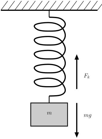
Let us consider a Hookean spring as an easy physical system (c.f., e.g., [LL81], [Bra79, Section 2.6]) and let us look at the forces occurring within this system. This example is also important for further discussions later in this thesis (see page 19 for the energetic approach to the spring; see Section 4.2 for application within the micro-macro model). Figure 3.1 shows a spring, of which one end is

m _mg

[image:21.595.219.395.361.599.2]

Fk

Figure 3.1: Mass attached to a Hookean spring

(22)

spring. This means that

F=−kx

for some material parameterk >0. The negative sign is due to the fact that the exerted force is in opposite direction to the displacement1_.

When the system moves up and down, the forceF is described by Newton’s law

F=ma, where the acceleration is a=xtt. Plugging force and acceleration into

the equation above yields

mxtt+kx= 0.

Now, one can solve this ordinary differential equation (with suitable initial con-ditions) to obtain the trajectories for the movement of the spring.

Moreover, we can add a term representing damping (due to friction; assumed to be linear in the velocity) within the system, so we end up with the differential equation

mxtt+γxt+kx= 0,

where γ >0 is the coefficient of the damping and xt is the velocity of the lower

end of the spring.

Now we consider the energetic approach. This leads to the same equation for the Hookean spring. To this end, we introduce the framework and the underlying principles first and come back to the spring at the end of Section 3.1.

3.1 General Approach

In 1873 and 1931, Lord Rayleigh (John William Strutt) and Lars Onsager, re-spectively, published works ([Str73], [Ons31a, Ons31b]) where they developed the general energetic variational framework (c.f. [Liu11], [HKL10]). This approach is based on the following concepts that are outlined below: energy dissipation law, least action principle, maximum dissipation principle, and Newton’s force balance law.

3.1.1 Energy Dissipation Law

The starting point for the energetic variational framework is the energy dissipa-tion law (c.f. [HKL10]),

d dtE

total_{+ ∆ = 0} _⇐⇒ d

dtE

total₌₋_∆, _(3.1) 1

(23)

where the total energy Etotal includes both kinetic and free internal energy, and ∆ is the dissipation functional (here this is equal to the entropy production, see (3.3), which is modeled as a quadratic function of certain rates such as the velocityxt).

The energy dissipation law (3.1) states that (in isothermal situations) the total energy is conserved over time (this is when ∆ = 0), unless the energy is dissipated into ∆.

Equation (3.1) can be derived from the first and second law of thermodynamics. The first law states that the rate of change of the kinetic energy K plus the internal energy U is due to the rates of change of workW and heatQ, so

d(K+U) dt =

dW

dt + dQ

dt . (3.2)

In other words, the first law of thermodynamics states that energy can only be changed by applied work and heat, so this is the conservation of energy. The second law is given in the isothermal case, i.e., when temperature is not time-dependent, by

TdS dt =

dQ

dt + ∆, (3.3)

whereT is the temperature,S is the entropy and ∆≥0 is the entropy production equal to the dissipation in (3.1) which is always nonnegative.

Now, we subtract (3.3) from (3.2) and find that (in the isothermal case)

d

dt(K+U −TS) = dW

dt −∆, (3.4)

whereF :=U −TS is the Helmholtz free energy andK+F is equal to the total energy Etotal. Thus, if no external forces are applied, i.e., if d_dtW = 0, the above expression yields the energy dissipation law (3.1).

Next we describe the energies of a system and make use of the energy dissipation law. Therefore, it is necessary to set up corresponding energy and dissipation functionals for the system. Then we derive differential equations of motion for the system. How this is done is described in the following sections.

3.1.2 Least Action Principle

We distinguish two different types of systems, on the one hand,Hamiltonian sys-tems, also referred to asconservative systems, and, on the other hand,dissipative systems.

As the name implies, energy is dissipated within the latter systems, while energy is conserved withinHamiltonian systems. Thus, the energy dissipation functional for such a system is identically zero.

(24)

the particles are moving from position x(X,0) at timet= 0 to position x(X, t∗) at time t = t∗. In particular, these trajectories of particles X are those which minimize the action functional defined below. Since we look only at one particle X, we write x(t) instead of x(X, t) here.

Definition 13. Let L = K − F be the Lagrangian function of a conservative system, where K is the kinetic and F is the free energy, depending on x(t) and the velocity xt(t). Then the action functional for this system is defined by

A(x(t)) :=

Z t∗

0

L(x(t), xt(t)) dt. (3.5)

The least action principle states that one can obtain the equation of motion for a Hamiltonian system by taking the variation of the action functional with respect to the flow mapsx(t) =x(X, t). To this end, we consider a variation x(t) +εy(t) of the minimizing trajectory x(t) for ε∈(−ε₀, ε₀),ε₀>0, andy(t) an arbitrary smooth and compactly supported test function.

Since x(t) is a minimizer of A(x(t)), the functionε7→A(x(t) +εy(t)) must have a minimum point in ε= 0. Hence, we calculate (assumingL of class C2)

0 = d dε

ε=0

A(x+εy)

= d dε

ε=0

Z t∗

0

L(x+εy, xt+εyt) dt

=

Z t∗

0

∂L ∂x(x, xt)

·y+

∂L ∂(xt)

(x, xt)

·ytdt

=

Z t∗

0

∂L

∂x(x, xt)− d dt

∂L ∂(xt)

(x, xt)

·y dt.

The last step is an integration by parts with respect to t. Since this is true for any y, by the fundamental lemma of the calculus of variations (see, e.g., [JLJ08, Lemma 1.1.1]) the following equation holds:

∂L

∂x(x, xt)− d dt

∂L ∂(xt)

(x, xt)

= 0. (3.6)

This is the so-called Euler-Lagrange equation or equation of motion and a nec-essary condition for the minimizing trajectories.

Moreover, the equation of motion of the conservative system gives the conserva-tive force. So, the principle of least action can be interpreted as the manifestation of the general rule ([Liu11], [HKL10])

δEtotal= forceconservative·δx,

(25)

3.1.3 Maximum Dissipation Principle and Force Balance

The maximum dissipation principle, however, leads to the dissipative force for a (dissipative) system. This is done by variation of the dissipation functional (in fact, 1₂∆ is used here, since ∆ is said to be quadratic in the rates, so the force is linear in the respective rates) with respect to the rate such as the velocity:

δ

1 2∆

= forcedissipative·δxt.

So, by the least action principle and the maximum dissipation principle we obtain all the forces for the system we consider.

The final step is to combine these forces with Netwon’s force balance law. The law states that all forces, both conservative and dissipative in kind, added up is equal to zero, or alternatively, “actio” is equal to “reactio”:

forceconservative= forcedissipative.

After we obtained the conservative and dissipative forces, the force balance yields the differential equation of motion for the entire system.

3.1.4 Hookean Spring Revisited

We now come back to the example from the beginning of this chapter, the Hookean spring. Again, x denotes the displacement of the lower end of the spring from its equilibrium position. Firstly, we have a look at the energies of the system. The kinetic energy is given by

K= 1 2mx

2 t,

and the free energy is given by the elastic energy

F = 1 2kx

2_.

Secondly, we give a dissipation term which is due to the damping / friction and depends on the velocity:

∆ =γx2_t.

Note that if the system would be frictionless, thus a conservative system, this function would be zero.

Equation (3.1) gives the following energy dissipation law for the Hookean spring:

d dt

1 2mx

2 t +

1 2kx

2

(26)

From here we can now derive the force balance law we found at the beginning of this chapter using energy variation. Therefore, we set up the action functional A(x) and take the variation with respect tox. The Action is given by

A(x) =

Z t∗

0

1 2mx

2 t−

1 2kx

2

dt.

We can use the Euler-Lagrange equation (3.6) from above, so with the Lagrangian functionL= 1₂mx2_t− 1₂kx2 we get immediately

−mxtt−kx= 0. (3.7)

This is exactly the conservative force for the Hookean spring.

Next we treat the dissipative part, hence, we calculate the variation of 1₂∆ with respect to the velocity. To this end, let yt be a smooth test function:

0 = d dε

ε=0

1

2∆ (xt+εyt) = d dε

ε=0

1

2γ(xt+εyt)

2

= (γxt·yt).

Since this equation must hold for anyyt, this yields the dissipative force and the

equation

γxt= 0. (3.8)

Now we have both the dissipative part (3.8) and the Hamiltonian part (3.7) of the system. The equation for the entire system then comes from Newton’s force balance law forceconservative= forcedissipative:

−mxtt−kx=γxt

or equivalently

mxtt+kx+γxt= 0. (3.9)

This is exactly the equation we obtained earlier by looking directly at the forces exerted on the spring. For this example, however, the energetic approach seems to be quite complicated. As already pointed out in the introduction, the fact that for more complex systems energy terms are relatively easy to establish, that force components within systems are not counted twice and, one of the most important ones, that it is a natural way of combining effects on different scales, are advantages of the energetic variational approach over the force-based approach (c.f. [EHL10]). This gets more important for systems which are not as easy as the Hookean spring.

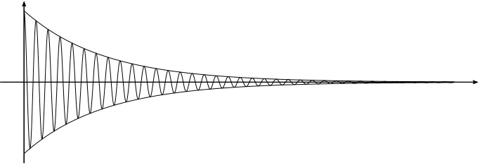
Remark 14. Equation (3.9) gives a good insight into how the dynamics of the system behave either near initial data, i.e., the short time behavior, or near equi-librium, i.e., the long time behavior.

In Figure 3.2 one particular solution of the damped spring equation (3.9)

(27)

witha >0, b:=−₂γ_m, c:=

q

k m−

γ2

4m2, x(0) =a, and the damping term

±aexp(bt)

are sketched.

The long time behavior, this is whentis very large, is governed by the dissipative part: It is obvious that

lim

t→∞|x(t)−aexp(bt)|= 0,

so the solutionx(t) behaves almost likeaexp(bt)for larget, which is the damping from the dissipative part γxt = 0 (c.f. (3.8)), and the oscillations are

approxi-mately negligible.

On the other hand, the short time is reflected by the Hamiltonian part, when the damping is negligible: For t >0 small, we have that exp(bt)≈1 and thus

x(t)≈acos(˜ct),

with˜c:=qk

m, which is a solution of the Hamiltonian part−mxtt−kx= 0 (c.f.

[image:27.595.139.482.401.521.2]

(3.7)). So the damping is negligible near initial data in an approximation. This concept is again relevant later on when we talk about the micro-macro model in Section 4.2.

Figure 3.2: Near initial data vs. near equilibrium dynamics

3.2 Simple Solid Elasticity and Fluid Mechanics

In this section we derive the equation of motion for systems describing simple solid or fluid materials by a given energy law. Here simple refers to a system which is either a solid or a liquid.

(28)

Example 15. Consider the energy law d dt Z ΩX 0 1

2ρ0(X)|xt(X, t)|

2₊1

2H ∂x(X, t) ∂X 2 dX !

= 0, (3.10)

where ρ0(X) is the mass density in the Lagrangian coordinate system (note that

the integral is taken over the reference configuration ΩX

0 ) and H is a constant.

The notion |A|2 for A ∈ Rn×n _{is defined as} _|A|2 := A : A with the double-dot product defined in Appendix A.1

Clearly, the first term is the kinetic energy, the second is the internal energy due to elastic effects where the deformation gradient is used.

Since the system is conservative (because the time-derivative of the total energy is zero, so energy is conserved), we only need to look at the least action principle. Therefore, we obtain the action for the system:

A(x(X, t)) =

Z t∗

0

Z

ΩX

0

1

2ρ0(X)|xt(X, t)|

2₋1

2H ∂x(X, t) ∂X 2 dX dt.

Now we take the variation of the action with respect tox. Here, the energy has an integral form and the internal energy depends on the deformation gradient, too. The calculus of variations tells us that this leads to the Euler-Lagrange equation for the integrand of the action, L(x, xt,_∂X∂x) (assuming L of class C2,

and bounded).

In addition to the dependence of the Lagrangian function on x and xt, which

leads to the Euler-Lagrange equation (3.6), we also consider the dependence on the deformation gradient _∂X∂x. The Euler-Lagrange equation is then given by

∂L(x, xt,_∂X∂x)

∂x −

d dt

∂(xt)

!

− ∇X ·

∂ _∂X∂x

!

= 0. (3.11)

Since L does not depend on x itself in this particular example but only on the spatial and time derivatives of the flow map, the following equation is obtained:

−ρ0(X)xtt(X, t) +H∇X ·

∂x(X, t) ∂X = 0

⇐⇒ρ0(X)xtt(X, t) =H∇X· ∇Xx(X, t).

If we embrace a shorter notation and use the Laplacian ofxas ∆Xx=∇X·∇Xx,

we obtain the wave equation

ρ0(X)xtt =H∆Xx. (3.12)

Remark 16. In the example we looked at a special case of elasticity,

(29)

which is called the case of linear elasticity. If we consider the general case, equation (3.12) changes to a nonlinear wave equation

ρ₀(X)xtt =∇X ·W_F_e(Fe). (3.13)

This equation is similar to (3.16) where we consider a fluid material in the La-grangian coordinate system.

The second example is again a Hamiltonian system. This time, however, a fluid is described and the Eulerian description is used.

Example 17. Consider the energy law

d dt

Z

Ωx t

1

2ρ(x, t)|u(x, t)|

2₊_{w(ρ(x, t))} _dx

!

= 0, (3.14)

whereρ(x, t)is the mass density in the Eulerian coordinate system (note that the integral is taken here over the deformed configuration Ωx

t),u is the velocity and

w is an internal energy density depending on the mass density.

Again, this system is conservative, so we only need to use the least action prin-ciple. However, the action functional incorporates an integral over the reference configurationR_ΩX

0 · · ·

dX since the variation is taken with respect to x.

Therefore, we need to write the energy law (3.14) in terms of the Lagrangian coordinate system first.

But, in addition to the simple coordinate change in the energy law, we also need information about how the mass densityρ(x, t) changes under the transformation of the coordinate system. Thus, we have to consider Proposition 12.

Since we do not have any incompressibility condition, the general kinematic as-sumption of mass transport holds, this is

ρt+∇x·(uρ) = 0

in the Eulerian coordinate system (as stated in equation (2.5)) or

ρ(x(X, t), t) = ρ0(X) detFe

in the Lagrangian coordinate system (as stated in equation (2.6)). With this additional assumption we are able to transform the integral and set up the cor-responding action functional (for brevity, we useJ = detFe):

A(x(X, t)) =

Z t∗

0

Z

ΩX

0

1 2

ρ0(X)

J |xt(X, t)|

2₋_w

ρ0(X)

J

J dX dt

=

Z t∗

0

Z

ΩX

0

1

2ρ0(X)|xt(X, t)|

2₋_w

ρ0(X)

J

(30)

Thus, taking the variation (for any y(X, t) = ˜y(x(X, t), t) smooth with compact support) with respect tox yields

0 = d dε _ε =0

A(x(X, t) +εy(X, t)) = d dε _ε =0

A(x+εy)

=d dε ε=0

Z t∗

0

Z

ΩX

0

1

2ρ0(X)|xt+εyt|

2

−w ρ0(X) det∂(x_∂X+εy)

!

det∂(x+εy) ∂X

dX dt

=

Z t∗

0

Z

ΩX

0

ρ0(X)xt·yt−

d dε _ε =0

w ρ0(X) det∂(x_∂X+εy)

!! · det ∂x ∂X

−w ρ0(X) det_∂X∂x

! · d dε ε=0

det∂(x+εy) ∂X

dX dt

(∗)

=

Z t∗

0

Z

ΩX

0

ρ0(X)xt·yt−wρ

ρ0(X)

J

·

−ρ0(X)

J2

·J·tr

∂X ∂x ∂y ∂X ·J −w

ρ0(X)

J

·J·tr

∂X ∂x ∂y ∂X dX dt,

where the formula for the derivative of the determinant from Lemma 9 is used at (∗). Next, we integrate by parts with respect to time which then yields 0 =

Z t∗

0

Z

ΩX

0

−ρ0(X)

J xtt·y·J +

wρ

ρ0(X)

J

·ρ0(X)

J −w

ρ0(X)

J ·tr ∂X ∂x ∂y ∂X

·J dX dt

=

Z t∗

0

Z

Ωx t

−ρ(x, t)

d dtu(x, t)

·y˜

+ (wρ(ρ(x, t))·ρ(x, t)−w(ρ(x, t)))·(∇x·y)˜ dx dt

=

Z t∗

0 Z Ωx t −

ρ(x, t)d

dtu(x, t) +∇x wρ(ρ(x, t))·ρ(x, t)−w(ρ(x, t))

·y dx dt˜

=

Z t∗

0 Z Ωx t −

ρ(x, t)(ut+u· ∇xu) +∇xp(x, t)

·y dx dt,˜

where we integrate by parts with respect tox in the second to last step.

Furthermore, the definition p(x, t) := wρ(ρ(x, t))·ρ(x, t) −w(ρ(x, t)) for the

pressure is used in the last step (equation of state). From the above calculation we get the equation of motion as ρ(ut+u· ∇xu) +∇xp= 0 and thus we obtain

the following system of equations:

    

ρt+∇x·(uρ) = 0

ρ(ut+u· ∇xu) +∇xp= 0

p=wρ(ρ)·ρ−w(ρ),

(31)

where the first equation is the Euler equation from the conservation of mass, the second equation is the equation of motion, and the last is the equation of state. System (3.15) describes an isentropic fluid, i.e., a fluid with constant entropy, if we assume, that there is no heat applied (d_dtQ = 0). Since the dissipation ∆ is equal to zero in (3.14), from the second law of thermodynamics (3.3) follows that (assumingT 6= 0)

dS

dt = 0,

so the entropy is constant.

Remark 18. The kinetic energy has the same form in both Lagrangian and Eulerian description, in the sense that it is linear in the density and quadratic in the velocity. This can be easily seen from a straightforward calculation using Proposition 12:

Z

ΩX

0

1

2ρ0(X)|xt(X, t)|

2 _dX ₌

Z

ΩX

0

1 2

ρ₀(X)

detFe|xt(X, t)|

2_·_det_{F dX}_e

=

Z

Ωx t

1 2

ρ₀(X)

detF |u(x, t)|

2 _dx

=

Z

Ωx t

1

2ρ(x, t)|u(x, t)|

2 _dx,

where we see that the determinants of the deformation gradient vanish when changing coordinates. However, this is not the case for the free energy in Example 17:

Z

Ωx t

w(ρ(x, t)) dx=

Z

ΩX

0

w

ρ0(X)

detFe

detF dX.e

Remark 19. In general, the free energy describing fluids only depends on the determinant of the deformation gradient detFe.

On the other hand, the free energy for solid materials can depend on the defor-mation gradient Fe itself as seen in Example 15.

(32)

3.3 Change of Coordinate Systems

We considered solid materials and used the Lagrangian coordinate system, for fluid materials we used the Eulerian description. Now we take a look at how the formulae change when we use the description the other way round, i.e., Eu-lerian coordinates for solids and Lagrangian coordinates for fluids. This gives us the possibility to choose the best description for certain models which is use-ful, e.g., to combine frameworks that are a priori defined for different coordinate systems.

Since the kinetic energy takes the same form in both Lagrangian and Eulerian coordinate system (see Remark 18), we only consider the free energy density for a fluid material. We have

Z

Ωx t

w(ρ(x, t)) dx=

Z

ΩX

0

Φ(F)e dX,

where we define Φ(Fe) :=w

ρ0(X) detFe

detFe

, and the least action principle (where we include the kinetic energy again, of course) yields the equation

ρ0(X)xtt =∇X ·ΦFe(Fe), (3.16)

which is actually a nonlinear wave equation as in the solid case (also Lagrangian coordinate system) considered above where (3.13) is obtained.

To consider solid elastic materials in the Eulerian coordinate system, we first look at the variation of the action corresponding to

d dt

Z

ΩX

0

1

2ρ0(X)|xt(X, t)|

2₊_W₍_F_e₎ _dX

!

= 0, (3.17)

(33)

Eulerian coordinate system at a certain step:

0 = d dε ε=0

A(x+εy)

= d dε ε=0

Z t∗

0

Z

ΩX

0

1

2ρ0(X)|xt+εyt|

2₋_W

∂(x+εy) ∂X

dX dt

=

Z t∗

0

Z

ΩX

0

ρ0(X)xt·yt−WFe(Fe) :

∂y ∂X dX dt =

Z t∗

0

Z

ΩX

0

−ρ0(X)

J xtt·y·J−WFe(Fe) : (∇Xy) dX dt

=

Z t∗

0

Z

Ωx t

−ρ(x, t)(ut+u· ∇xu)·y˜−

1

J ·WF(F)

: (∇xy˜·F) dx dt

=

Z t∗

0

Z

Ωx t

−ρ(x, t)(ut+u· ∇xu)·y˜−

1

J ·WF(F)·F

T

: (∇xy)˜ dx dt

=

Z t∗

0

Z

Ωx t

−ρ(x, t)(ut+u· ∇xu)·y˜+∇x·

1

J ·WF(F)·F

T

·y dx dt˜

=

Z t∗

0 Z Ωx t −

ρ(x, t)(ut+u· ∇xu)− ∇x·

1

J ·WF(F)·F

T

·y dx dt.˜

Here we use the product A : B from Appendix A.1 for n×n-matrices and the fact that the derivative of the scalar-valued function W(Fe) with respect to its argument Fe is again a matrix of dimension n×n. For details concerning the derivative _dεdW∂(x_∂X+εy)from above, see Appendix A.2.

The integration by parts in the second to last step is explained in detail in Appendix A.4.

Thus, we obtain the equation of motion for solid material in the Eulerian de-scription ρ(x, t)(ut+u· ∇xu) = ∇x· _J1 ·WF(F)·FT

. We add the kinematic assumptions and obtain the entire system

    

ρt+∇x·(uρ) = 0 ∂F

∂t +u· ∇xF =∇xu·F

ρ(ut+u· ∇xu) =∇x· _J1 ·WF(F)·FT

,

(3.18)

where the first equation is the general conservation of mass (c.f. (2.5)) and the second is the chain rule (2.3). The last equation is the wave equation in the Eulerian coordinate system.

Remark 20. The quantity W_F_e(Fe) that comes up in Remark 16 is called the Piola-Kirchhoff stress (c.f. [TM11, Section 8.1.2]). The corresponding quantity in the Eulerian description is the so-called Cauchy-Green stress _J1 ·WF(F)·FT

(34)

3.4 Addition of Dissipation

In Sections 3.2 and 3.3 we considered only Hamiltonian systems of fluid and solid materials. Now we add dissipation terms to the fluid and solid models from above (c.f. energy dissipation law (3.1)). At first, we look at the energy law describing a solid material:

d dt

Z

ΩX

0

1

2ρ0(X)|xt(X, t)|

2₊_W₍_F_e₎ _dX

!

=−

Z

ΩX

0

η(x(X, t), t)|xt(X, t)|2 dX,

where

∆ =

Z

ΩX

0

η(x(X, t), t)|xt(X, t)|2 dX (3.19)

is the dissipation with a chosen dissipation coefficient η that depends on spatial and time variables.

This is one ansatz in modeling the dissipation functional. However, after the discussion of this particular dissipation in the Eulerian coordinate system for a fluid, we see another ansatz involving the spatial gradient and the divergence of the velocity u.

The dissipation is chosen to be quadratic in the rates, so the dissipative force that is derived from the dissipation by taking the variation of 1₂∆ with respect to the velocity is linear in the rates. For the chosen dissipation ∆ this yields

forcedissipative =η(x(X, t), t)xt(X, t) =ηxt.

So, by Newton’s force balance law, we can extend the equation of motion for the system (c.f. Remark 16) by a dissipative term, thus

ρ₀(X)xtt=∇X ·WFe(Fe)−ηxt.

This is a damped wave equation. If we look at the same system in the Eulerian coordinate system, we obtain by extending (3.18)

    

ρt+∇x·(uρ) = 0 ∂F

ρ(ut+u· ∇xu) =∇x· _J1 ·WF(F)·FT

−_J1ηu, since we take the variation with respect to u of

1 2∆ =

1 2

Z

ΩX

0

η(x(X, t), t)|xt(X, t)|2 dX =

1 2

Z

Ωx t

η(x, t)

J |u(x, t)|

2 _dx.

(35)

Remark 21. The damping considered in (3.19) is called Darcy’s damping.

Concerning Example 17 for a fluid system, we can also add dissipation like Darcy’s damping. This leads to the Euler-Darcy system

    

ρt+∇x·(uρ) = 0

ρ(ut+u· ∇xu) +∇xp=−ηu

which is extended from (3.15) using the dissipation ∆1 =R_Ωx

t η(x, t)|u(x, t)|

2 _dx,

where we choose the dissipation coefficient η(x, t) directly in the Eulerian coor-dinate system.

Moreover, we could also choose dissipation terms involving the spatial gradient and the divergence ofu. This is used in modeling viscosity. We consider

∆2=

Z

Ωx t

µ1(x, t)|∇xu|2+µ2(x, t)|∇x·u|2 dx, (3.20)

where µ₁, µ₂ are viscosity constants. The name “constants” is due to the fact that they are constant for a particular material. However, they can depend onx and t(and are assumed to do this for now).

If we incorporate dissipation ∆2, we can calculate the dissipative force through

0 = d dε

ε=0

1

2∆2(u+εv)

= d dε

ε=0

Z

Ωx t

1

2µ1(x, t)|∇xu+ε∇xv|

2₊1

2µ2(x, t)|∇x·u+ε∇x·v|

2 _dx

=

Z

Ωx t

µ1(x, t)∇xu:∇xv+µ2(x, t)(∇x·u)(∇x·v) dx

=

Z

Ωx t

−∇x·(µ1(x, t)∇xu)− ∇x(µ2(x, t)∇x·u)

·v dx,

where v is any test function with compact support, and the system (3.15) be-comes

    

ρt+∇x·(uρ) = 0

ρ(ut+u· ∇xu) +∇xp=∇x·(µ1∇xu) +∇x(µ2∇x·u)

which describes a viscous fluid.

Now we have a look at the first viscosity term and transform the integral into the Lagrangian coordinate system. We get

Z

Ωx t

µ1(x, t)|∇xu|2 dx=

Z

ΩX

0

(36)

The transformation of the gradient can be easily seen by going a bit more into detail. For 1≤i, j≤nwe have that

(∇Xxt(X, t))ij =

∂xi_t(X, t) ∂Xj =

∂ui(x(X, t), t) ∂Xj

= ∂u

i_{(x(X, t), t)}

∂xk

∂xk ∂Xj =

(∇xu)Fe

ij, (3.21)

where we use the Einstein summation convention and the chain rule. Hence

∇xu=∇Xxt(X, t)Fe−1. (3.22)

From here we see that the expression gets much more complicated, since the deformation gradient comes into play, too, which yields the following remark.

Remark 22. Viscosity is convenient to use with the Eulerian coordinate system.

3.5 Consideration of Incompressibility Condition

From Definition 6 and Proposition 7 we recall the mathematical description of incompressibility. In theLagrangian coordinate system it is

detFe≡1, (3.23)

in theEulerian coordinate system it is

∇x·u= 0. (3.24)

Note that (3.23) is a nonlinear constraint for the flow map, while (3.24) is linear, so, if we do a variation with respect to the velocity uin the Eulerian coordinate system under incompressibility conditions, we can use functions u+εv which satisfy∇x·(u+εv) = 0.

On the other hand, if we do a variation with respect tox, which is the case when applying the least action principle, the difficulty is that det_∂X∂x +ε_∂X∂y ≡ 1 does not hold if det_∂X∂x ≡1 holds.

In this case, we use volume preserving diffeomorphisms to perform the variation, i.e., functionsxε such that

x0 =x and dx

ε

dε

ε=0

:=y and ∀ε: detFeε = det∂x

ε

∂X ≡1. (3.25)

The nonlinear constraint, however, leads to a divergence condition fory(X, t) = ˜

y(x(X, t), t) similar to (3.24) in the Eulerian coordinate system. Indeed, from (3.25) we get

0 = d dε

ε=0

det∂x

ε

∂X

= detFe·tr

e

F−1 d dε

ε=0

∂xε

∂X

= tr

n

X

k=1

∂Xk

∂xi

∂yj

∂Xk

!

(37)

Equation (3.26) provides us with a necessary condition which is crucial for cal-culating, e.g., first variations if incompressibility holds.

Now we look at a problem under incompressibility condition. We consider the energy law

d dt

Z

Ωx t

1

2ρ(x, t)|u(x, t)|

2 _dx

!

=−

Z

Ωx t

µ(x, t)|∇xu|2 dx, (3.27)

which is a simple viscous fluid.

To put the simple part first, we start with the variation of the right-hand side. Here, we useu+εv since we are in the Eulerian coordinate system and∇x·(u+

εv) = 0 holds for any compactly supported and smooth test functionvsatisfying

∇x·v= 0. The calculation is similar to the one using ∆2 in the previous section;

we obtain:

0 = d dε

ε=0

1

2∆ (u+εv) =

Z

Ωx t

−∇x·(µ(x, t)∇xu)

·v dx. (3.28)

This is a crucial point: In the compressible case, the equation of motion is

−∇x·(µ(x, t)∇xu) = 0 since the field v is arbitrary.

Now the fieldvis divergence free, hence we useWeyl’s decomposition orHelmholtz’ decomposition of a vector field (c.f. [DL00, Chapter IX, Section 1, Propostion 1]; we omit the proof for brevity):

Proposition 23. If a vector field w ∈ L2(Ω,Rn₎ _{is orthogonal to all smooth}

divergence free vector fields with compact support, thenwhas gradient form, i.e.,

w=∇p for somep∈W1,2(Ω,Rn₎_.

Thus, we obtain the following equation of motion for the dissipative part:

−∇x·(µ∇xu) =∇xp2 (3.29)

withp₂ ∈W1,2_(Ω,_Rn_).

Now we turn to the Hamiltonian part. For the least action principle we use variations xε of x as described in (3.25) and (3.26) with y satisfying y(X,0) = y(X, t∗) = 0 for any X ∈ ΩX

0 . Due to incompressibility, the mass density is

(38)

we can calculate the variation of the action functional:

0 = d dε ε=0

A(xε) = d dε ε=0

Z t∗

0

Z

ΩX

0

1

2ρ0(X)|x

ε

t|2 dX dt

=

Z t∗

0

Z

ΩX

0

ρ0(X)

xε_t

ε=0 · d dε ε=0

xε_t

dX dt

=

Z t∗

0

Z

ΩX

0

ρ0(X)xt·ytdX dt

=

Z t∗

0

Z

ΩX

0

−ρ0(X)xtt·y dX dt

=

Z t∗

0

Z

Ωx t

−ρ(x, t)(ut+u· ∇xu)·y dx dt,˜

where the equality y(X, t) = ˜y(x(X, t), t) is used in the transformation of the in-tegral in the last step. We can apply Proposition 23 again because ˜yis divergence free due to (3.26), hence, for somep1 ∈W1,2(Ω,Rn) we have

−ρ(x, t)(ut+u· ∇xu) =∇xp1. (3.30)

Putting both results (3.29) and (3.30) together (where we make use of the force balance law: forceconservative = forcedissipative) and adding also the kinematic

assumptions of incompressibility (c.f. (3.24)) and conservation of mass (2.5), we obtain the following system

    

∇x·u= 0

ρt+u· ∇xρ= 0

ρ(ut+u· ∇xu) +∇xp=∇x·(µ∇xu),

(3.31)

where we setp=p1−p2. This is the Lagrange multiplier for the incompressibility

constraint, reflecting both the Hamiltonian and the dissipative part of the system. This is a Navier-Stokes system for incompressible viscous fluids.

(39)

4 Modeling of Complex Fluids

In this chapter we discuss exemplary models for complex fluids. We use the en-ergetic variational approach and the mechanical tools explained in the previous chapters to derive differential equations from energy laws describing the phenom-ena within the materials.

Throughout this chapter we assume that the considered functions have enough regularity and the integrands are bounded, so the calculations are well-defined. We start with a rather general model of incompressible viscoelastic materials such as biological materials (e.g. muscles) or rubbers. Here we put several concepts together in order to generate one modeling framework to incorporate solid and fluid properties. After that we go down on a smaller scale to see where these properties come from: We study polymeric fluids through a micro-macro analysis in Section 4.2 to analyze the effect of polymers, which are surrounded by a fluid, onto the (macroscopic) fluid flow. In Section 4.3 we consider liquid crystals and study coupling effects with a fluid.

4.1 Incompressible Viscoelasticity

As the title “Incompressible Viscoelasticity” implies, we have incompressibility

first (c.f. (3.24)):

∇x·u= 0.

Secondly, there is some visco part, so we have viscosity (c.f. (3.20)), a property of fluid material, and something like

Z

Ωx t

µ|∇xu|2 dx,

whereµ > 0 is a viscosity constant which is assumed to be constant inx and t. Moreover, there is a third part,elasticity, so we need

Z

Ωx t

λW(F) dx,

with an elasticity density W(F) (c.f. (3.17)), incorporated with a relaxation pa-rameter λ >0.

(40)

In contrast to the previous chapter where we considered models for solid and fluid materials separately, we now take both fluid and solid properties together and create a unifiedviscoelastic framework.

This is also an approach to simplify the way we look at solid and fluid materials which is the idea of the viscoelastic model. However, special cases in terms of the choice of µ and λlead to the model of (incompressible) solid elasticity and the model of (incompressible) viscous fluids, respectively.

We establish the energy law for this model of incompressible viscoelasticity as follows: d dt Z Ωx t 1 2ρ|u|

2₊_λW_(F₎_dx₌₋

Z

Ωx t

µ|∇xu|2 dx, (4.1)

incorporating both solid (elasticity) and fluid (viscosity) properties. The action is given by

A(x) =

Z t∗

0

Z

ΩX

0

1

2ρ0(X)|xt(X, t)|

2₋_λW₍_F_e₎ _{dX dt,} _(4.2)

which is transformed into the Lagrangian coordinate system. Notice that J = detFe≡1 due to the incompressibility.

Now we calculate the variation of the action (4.2), where we use volume preserv-ing diffeomorphisms xε as characterized in (3.25) and (3.26) with y satisfying y(X,0) = y(X, t∗) = 0 for any X ∈ ΩX

0 , since we work under incompressibility

conditions (compare also the variation of (3.17), where is, however, neither any relaxation nor incompressibility):

0 = d dε ε=0

A(x+εy)

= d dε ε=0

Z t∗

0

Z

ΩX

0

1

2ρ0(X)|xt+εyt|

2₋_λW

∂(x+εy) ∂X

dX dt

=

Z t∗

0

Z

ΩX

0

ρ0(X)xt·yt−λWFe(Fe) :

∂y ∂X dX dt =

Z t∗

0

Z

ΩX

0

−ρ₀(X)xtt·y−λWFe(Fe) : (∇Xy) dX dt

=

Z t∗

0

Z

Ωx t

−ρ(x, t)(ut+u· ∇xu)·y˜−λ(WF(F)) : (∇xy˜·F) dx dt

=

Z t∗

0

Z

Ωx t

−ρ(x, t)(ut+u· ∇xu)·y˜−λ WF(F)·FT

: (∇xy)˜ dx dt

=

Z t∗

0

Z

Ωx t

−ρ(x, t)(ut+u· ∇xu)·y˜+λ∇x· WF(F)·FT

·y dx dt˜

=

Z t∗

0 Z Ωx t −

ρ(x, t)(ut+u· ∇xu)−λ∇x· WF(F)·FT

(41)

where the productA:B from Appendix A.1 is used. For details concerning the derivative _dεdW∂(x_∂X+εy)from the calculation above, see Appendix A.2.

The integration by parts in the second to last step is explained in detail in Appendix A.4.

At this stage we apply Helmholtz’ decomposition as in Proposition 23 and obtain for somep1 ∈W1,2(Ω,Rn)

ρ(ut+u· ∇xu)−λ∇x· WF(F)·FT

=−∇xp1, (4.3)

which yields the Hamiltonian part. For the dissipative part we look at the dissi-pation in the energy law (4.1):

∆ =

Z

Ωx t

µ|∇xu|2

dx,

where we perform the variation with respect to the velocity u. This variation, however, is the same as in (3.28). Again by Proposition 23, the calculations lead to the following equation of motion for the dissipative part (3.29):

−∇x·(µ∇xu) =∇xp2,

forp2 ∈ W1,2(Ω,Rn), or equivalently, since µ is assumed to be constant in this

model,

−µ∆xu=∇xp2. (4.4)

Equations (4.3) and (4.4) are brought together by the force balance law

forceconservative = forcedissipative which yields the entire equation of motion for

the macroscopic scale

ρ(ut+u· ∇xu) +∇xp=µ∆xu+λ∇x· WF(F)·FT

. (4.5)

wherep=p₁−p₂.

We now put the system’s equations together. To this end, we state the kinematic assumptions of incompressibility (c.f. (3.24)), the chain rule for the deformation gradient (2.3) and conservation of mass (c.f. (2.5) and part 2 of Proposition 11), and the equation of motion (4.5). We obtain the following system:

          

∇x·u= 0 ∂F

ρt+u· ∇xρ= 0

ρ(ut+u· ∇xu) +∇xp=µ∆xu+λ∇x· WF(F)·FT

.

(4.6)

(42)

What can be easily seen in system (4.6) and in the corresponding energy law (4.1) is that we can use the parameters λ and µ to choose the influence of elasticity and viscosity, respectively, within the model.

If we set µ = 0 and λ > 0, we get a model for incompressible solid elasticity as in (3.18). On the other hand, if we set λ = 0 and µ > 0, the model is for incompressible viscous fluids. We obtained this earlier in (3.31). Basically, we tear the fluid and solid properties apart again.

Now it is interesting to ask where solid and fluid properties come from and where these properties have their seeds in. For a particular example of fluids, this is discussed in the following section.

4.2 Micro-Macro Models for Polymeric Fluids

This section deals with physical phenomena that happen on an atomistic scale. The question that came up in the last section, where do solid and fluid properties come from, shall be discussed to some extent.

What we do here, is the so-called multiscale modeling. This means, we look at phenomena occurring at different length and/or time scales [TM11, Chapter 10]. To make clear what is meant by different scales, we take a look at different length scales in some copper material like a coin (c.f. [TM11, Section 1.1]).

On the largest scale, i.e., what is visible to the naked eye at a 1mm scale, we see a solid coin made from hard material.

When we go down to finer scales at micrometers and nanometers, we can observe certain structures and patterns.

Down at the ˚Angstrom length scale, we see the individual positions of the atoms. Concerning time scales, we see that for the coin as a whole piece of copper at the largest scale, motion and deformation processes like creep and fatigue may take years. On the other hand, down at the finest scale, the vibration of atoms takes place on a femtosecond scale ( 1fs = 0.000 000 000 000 001s = 10−15s).

In our modeling, however, we only use two scales: a macroscopic or “coarse” scale (largest) and a microscopic or “fine” scale. We assume that these scales commu-nicate through averaging from micro to macro and through interpolation from macro to micro. Moreover, we assume separation of scales, i.e., if we know what happens on both the microscopic and the macroscopic scale, we know everything that happens in between.

We consider a domain Ωx

t ⊂R3 in the Eulerian coordinate system on the

macro-scopic scale. On the fine scale we consider the configuration space R3, i.e., we look at the polymer molecules as end-to-end vectors Q ∈ R3_{. These polymers}

are modeled as small springs, see Figure 4.1. Additionally, we need a distri-bution function f(Q, t) for the polymers satisfying RR3f(Q, t) dQ = const, and

lim|Q|→∞f(Q, t) = 0 and lim|Q|→∞∇Qf(Q, t) = 0 for allt≥0. Then we perform

some averaging over the fine scale which leads to the effect onto the macroscopic scale. So, a pointx∈Ωx

t represents the properties of a bunch of polymers in the

(43)

Q∈R3

Ωx t

[image:43.595.224.394.72.225.2]

x

Figure 4.1:Microscopic vectors acting as springs in the fine scale, averaged to the macroscopic scale

4.2.1 Microscopic Scale

We start with the microscopic scale, where we look at the polymer end-to-end vectors Q ∈ R3 as springs. From previous chapters we know the equation of motion governing the spring (3.9). We use a general elastic potential U(Q) (c.f. [LLZ07, Section 2]) and obtain

Qtt+γQt=−∇QU,

whereγ >0 is a damping constant. We consider situations where the motion on the fine scale is much faster than on the macroscopic scale. So for the microscopic behavior, we can say that we are only interested in the long time dynamics (c.f. Remark 14). Thus, we neglect the oscillation part Qtt which yields

γQt=−∇QU (4.7)

as a governing equation. This dynamical behavior is calledgradient flow or near equilibrium dynamics.

We consider now the distribution functionf(Q, t) from above. Like for the mass density or mass distribution function ρ(x, t) considered in Section 2.4, we can establish the transport equation ft+∇Q·(Qt f) = 0 (c.f. equation (2.5)) since

the number of particles is conserved over time.

With the gradient flow equation (4.7) the transport equation forf becomes

ft− ∇Q·

1

γ∇QU f

= 0.

Now we add thermal fluctuations to the gradient flow (4.7) by adding an isotropic Brownian motion and obtain

dQ=−1

(44)

Here, Wt is a regular Wiener process representing the Brownian motion and

σ = kT, where k is the Boltzmann constant and T is the temperature (c.f. [LLZ07]). When It¯o’s lemma from stochastic differential calculus is applied, we see that the distribution functionf(Q, t) satisfies

ft=∇Q·

1

γ∇QU f

+σ

2

2 ∆Qf, (4.9)

which is the Fokker-Planck equation [PB99, Section 3.5]. Furthermore, it holds that f ≥ 0 and the equilibrium distribution is given by f = Cexp−_γσ22U

[LLZ07, Section 2].

We define the free energyRR3A(f)dQwith the free energy density (c.f. [EHL10])

A(f) = σ

2

2 flnf+ 1 γU f.

The term σ₂2flnf is called Gibbs entropy and corresponds to the transport of the molecules through Brownian motion. The second term represents the elastic energy density due to the spring model of the polymers.

Now we can use (4.9) (in the third step) to derive the following dissipative energy law (we assume thatf and U are chosen in the way that the boundary terms (as

|Q| → ∞) vanish in the integration by parts): d dt Z R3 σ2

2 flnf+ 1 γU f

dQ = Z R3 σ2

2 (ftlnf+ft) + 1 γU ft

dQ = Z R3 σ2

2 (lnf+ 1) + 1 γU

ft dQ

=

Z

R3

σ2

2 (lnf+ 1) + 1

γU ∇Q·

1

γ∇QU f

+σ

2

2 ∆Qf

dQ = Z R3 σ2

2 (lnf+ 1) + 1 γU

∇Q·

1

γ∇QU f + σ2

2 ∇Qf

dQ =− Z R3 ∇Q σ2

2 (lnf+ 1) + 1 γU · 1

γ∇QU f + σ2

2 ∇Qf

dQ =− Z R3 ∇Q σ2

2 (lnf+ 1) + 1 γU · 1

γ∇QU + σ2

2 1 f∇Qf

f dQ

=−

Z

R3

f∇Q

σ2

2 (lnf + 1) + 1 γU

· ∇Q

σ2

2 (lnf+ 1) + 1 γU dQ =− Z R3 f ∇Q σ2

2 (lnf+ 1) + 1 γU

2

Mathematical Modeling of Complex Fluids