Efficient pointcut projection

(1)

MASTER THESIS

EFFICIENT

POINTCUT

PROJECTION

Remko Bijker

COMPUTER SCIENCE

SOFTWARE ENGINEERING GROUP

(2)

Software Engineering Group

University of Twente

Master thesis

Efficient pointcut projection

Author:

Remko Bijker

Supervisors:

Dr.-Ing. ChristophBockisch

Dr. Pim van den _Broek

(3)

(4)

Abstract

Pointcuts in aspect-oriented programming languages specify run-time events which cause execution of additional functionality. Hereby, pointcuts typi-cally have a pattern-based static component selecting instructions whose execution triggers an event, e.g. a pattern that selects method-call instruc-tions based on the target method’s name. Current implementainstruc-tions realise identification of matching instructions by examining all instructions in the executed program and matching them against all patterns found in the pro-gram’s pointcuts. But such an implementation is slow. An optimised im-plementation is therefore highly desirable in run-time environments which support the dynamic deployment of aspects; slow pattern evaluation invari-ably causes a slowdown of the entire application.

The patterns used in pointcuts supported by current languages, i.e.

method, constructor, and field signatures, are well structured. In order

to speed-up pattern matching, this structure can be exploited, both to cre-ate indexes over the relevant instructions and to optimise the order in which the sub-patterns are evaluated. In this thesis we present background on pattern matching and outline two optimisation strategies. We furthermore present two case studies that survey signatures and patterns that actually occur in the real-world. This results in several heuristics that can improve the performance of matching patterns to instructions.

(5)

(6)

Contents

Chapter 1

Introduction

Aspect-orientation languages are means to reduce the maintenance costs for application components that cross-cut large parts of an application, e.g. logging.

This section will first define the terminology used in this thesis, after that the motivation and problem statement will be discussed.

The main contributions of Chapter 2, 4, and 5 are published in the proceedings of the VMIL workshop [4].

1.1

Terminology

In aspect-orientation there are different, sometimes opposite, terminologies. This section describes the terminology used in this report that is derived from [18]. The terminology is based on the one used for the ALIA4J frame-work [6].

Generic-function The logical grouping of functionality implementations which may all be executed as the result of executing a call-site. They apply to the same static context (have the same signature) but are applicable in different dynamic situations.

Pattern Description of a generic-function’s signature, e.g. a MethodPattern describes the signature of a method.

Context Run-time information about the program’s current call context, e.g. from which method it is called.

Atomic predicate A single test to execute at run-time.

Predicate A boolean formula of atomic predicates to execute at run-time.

(9)

Specialisation Association of a pattern, predicate and contexts.

Attachment A collection of specialisations associated with an action.

Projection of specialisation All call-sites of generic-functions where the signature of the called generic-function matches the pattern of the specialization.

1.2

Context and motivation

In aspect-orientation implementations there are different times in the deploy-ment of an application at which the needed support for can be applied [19].

Compile-time While compiling the application the compiler inserts the predicate evaluations and actions at every possible projection of the

specialisations. This generally requires no modifications to virtual

machines or loaders; all needed code is part of the application.

Load-time While loading the application an overridden loader inserts the predicate evaluations and actions at every possible projection of the specialisations. The modifications to the loader mean that there is a dependency on the workings of the virtual machine.

Run-time While running the application a hook is set at every possibly projection of the specialisations. This hook calls the predicate eval-uations and actions. The break points are implemented by either a modified virtual machine or via debugging hooks.

In all implementations one needs to match call-sites to attachments. One common optimisation is calculating what specialisation may match at any given call-site and insert only code to execute the actions for the matching attachments like AspectJ does. In this case adding the actions at compile-time is a disadvantage because even if an attachment is not activated the code has to be added. For load and run-time deployment one can omit the code to execute an action if the attachment the action belongs to is not activated, thus reducing the impact of the attachment.

Even if it is possible, there are many concepts in aspect orientation that cannot be determined at compile/load-time, which is where matching call-sites to an attachment has to be done at e.g. run-time. The trivial solution to this matching is using a list of specialisations that is searched for matches with the call-site the application’s execution is currently at. This can be optimised by using the non run-time dependent to determine which specialisations could possibly match at a given call-site.

(10)

1.3. Contents

matching call-sites to a specialisation. This study will put focus on a sur-vey of used patterns and call-sites as well as an implementation to test the actual merits of the proposed improvements in the ALIA4J framework.

1.3

The rest of this report is structured as follows: Chapter 2 describes the data model of the ALIA4J framework, which is the model that will be used for the examples. Chapter 3 explores the problem statement and sets the bound-aries for this study. Chapter 4 will discuss different possible optimisations using techniques from database query optimisation.

Chapter 5 discusses a survey of real world applications and patterns to determine how to apply the theory from the first chapters to improve the performance of implementation described in Chapter 6.

(11)

(12)

Chapter 2

Data model of ALIA4J

In ALIA4J’s high level design an attachment is associated with an action, schedule information which specifies relative ordering of actions, and a num-ber of specialisations. A specialisation is associated with a pattern, contexts and a predicate. This is visualised in Figure 2.1.

Attachment

Action Specialization ScheduleInfo

Context Predicate Pattern

AtomicPredicate

1..*

*

* _0..1

[image:12.595.160.388.371.518.2]

0..2

Figure 2.1: UML class diagram of an attachment in ALIA4J [6]

As mentioned earlier the main focus of this research lies on the patterns. The patterns are split into five categories which can be used to describe all the possible call-sites:

• Method pattern

• Constructor pattern

• Static initialiser pattern

• Field read pattern

(13)

These patterns have all been split up in sub-patterns that are finally used for matching, e.g. the constructor pattern only matches the (enclosing) class type, modifiers, parameters and exceptions sub-patterns. The sub-patterns are:

• Modifiers pattern Used to match the modifiers of a method,

con-structor or field that is accessed. Examples areprivate,public, but

alsostatic,final, and many more. It is possible to specify an inverse

modifier, e.g. notfinal.

• Type patternUsed to match the return, parameter or exception type of methods and exceptions or the type of a field. The type is matched by either its fully qualified class/primitive name or a wild card, e.g.

java.*for all classes in thejavapackage.

• Class type pattern Used to match the enclosing type of accessed methods, constructors, static initialisers and field patterns. It works the same as the type pattern, although primitive and array types are not allowed.

• Name patternUsed to match the name of a method or field. Match-ing can be done with exact matches or by means of regular expressions.

• Parameters patternUsed to match the parameters of a method or constructor. Matching is done by means of matching type patterns for the parameters including a wild card type that matches any number of parameters.

• Exceptions patternUsed to match the exceptions that a method or constructor have declared to be thrown. Matching is done by means of matching type patterns for the exceptions.

All sub-patterns have the possibility of performing logical algebra on a num-ber of sub-patterns, i.e. to negate the whole pattern, requiring matching multiple patterns or requiring one of a set of patterns to match.

2.1

Examples

To make the concepts of ALIA4J more concrete this section will show a number of examples, which will be used throughout this report to explain the different concepts important to the individual parts of this study.

Listing 2.1 shows a number of snippets from a hypothetical transport simulation game/model where cargo is moved by Vehicles, e.g. Trains and Busses, between stations. Their relationship is shown in Figure 2.2.

(14)

2.1. Examples

Vehicle

Train Bus

Station

Figure 2.2: UML class diagram of the example application used in this study

1 i n t e r f a c e V e h i c l e {

2 C a r g o G e t T r a n s p o r t e d C a r g o ();

3 int G e t A m o u n t ();

4 int G e t C a p a c i t y ();

5 v o i d C h a n g e A m o u n t ( int d e l t a _ a m o u n t )

6 }

7 s t a t i c int V e h i c l e :: A f t e r C r a s h ( T r a i n t , Bus b ) {

8 /* B u s s e s i m p l i c t l y t r a n s p o r t p a s s e n g e r s */

9 int c a s u a l t i e s = b . G e t A m o u n t ();

10 if ( t . G e t T r a n s p o r t e d C a r g o () == C A R G O _ P A S S E N G E R )

11 c a s u a l t i e s += t . G e t A m o u n t ();

12 r e t u r n c a s u a l t i e s ;

13 }

14 v o i d S t a t i o n :: M o v e C a r g o T o V e h i c l e ( V e h i c l e v ) {

15 C a r g o c = v . G e t T r a n s p o r t e d C a r g o ();

16 int w a i t i n g = t h i s . w a i t i n g _ c a r g o [ c ];

17 int c a p a c i t y = v . G e t C a p a c i t y () - v . G e t A m o u n t ();

18 int t o _ m o v e = min ( waiting , c a p a c i t y );

19 v . C h a n g e A m o u n t ( t o _ m o v e );

20 t h i s . w a i t i n g _ c a r g o [ c ] = w a i t i n g - t o _ m o v e

21 }

22 v o i d S t a t i o n :: M o v e C a r g o T o S t a t i o n ( V e h i c l e v ) {

23 C a r g o c = v . G e t T r a n s p o r t e d C a r g o ();

24 int t o _ m o v e = v . G e t A m o u n t ();

25 v . C h a n g e A m o u n t ( - t o _ m o v e );

26 t h i s . w a i t i n g _ c a r g o [ c ] += t o _ m o v e ;

27 }

28 s t a t i c v o i d V e h i c l e :: C o l l s i o n D e t e c t () {

29 ..

30 int c a s u a l t i e s = A f t e r C r a s h ( t , b );

31 ..

32 }

(15)

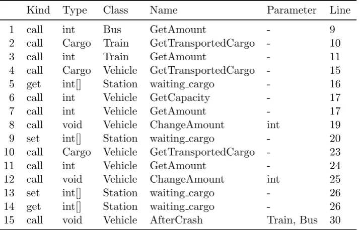
Kind Type Class Name Parameter

1 call * Vehicle+ Get* *

2 call Cargo * Get*

-3 call void Vehicle+ ChangeAmount *

4 call int Vehicle AfterCrash Train, Bus

5 set int[] Station waiting cargo *

Table 2.1: The patterns to match in the example application.

Kind Type Class Name Parameter Line

1 call int Bus GetAmount - 9

2 call Cargo Train GetTransportedCargo - 10

3 call int Train GetAmount - 11

4 call Cargo Vehicle GetTransportedCargo - 15

5 get int[] Station waiting cargo - 16

6 call int Vehicle GetCapacity - 17

7 call int Vehicle GetAmount - 17

8 call void Vehicle ChangeAmount int 19

9 set int[] Station waiting cargo - 20

10 call Cargo Vehicle GetTransportedCargo - 23

11 call int Vehicle GetAmount - 24

12 call void Vehicle ChangeAmount int 25

13 set int[] Station waiting cargo - 26

14 get int[] Station waiting cargo - 26

[image:15.595.145.503.291.520.2]

15 call void Vehicle AfterCrash Train, Bus 30

Table 2.2: The generic-function call-sites in the snippets from Listing 2.1.

Generic-function call-sites

1 2 3 4 5 6 7 8 9 10 11 12 13 14 15

P

atterns

1 X X X X X X X X

2 X X

3 X X

4 X

5 X X

(16)

2.1. Examples

means Vehicle or its sub classes, “-” means no parameters. For the “call” patterns the “Type” is the return type of the called function whereas it is the type of the (instance) variable for “set” patterns.

Table 2.2 lists the sites in the snippets. Some sites, e.g. call-sites 7 and 11, are the same when looking at only the pattern, however due to the a call-site being the place where a function is called, and not the (unique) function that is called, they are different. For brevity the modifiers information is omitted.

(17)

(18)

Chapter 3

Problem statement

The aim of this study is to determine what methods from different fields of software engineering can be used to improve the performance of matching call-sites to patterns. The focus lies on the algorithms and data structures that are used for efficiently matching call-sites to patterns. This matching should take the structure of the executed application into account, i.e. it should use matching heuristics based on the executed application.

On one hand the characteristics, including theoretical complexities and trade-offs, of the algorithms and data structures have to be evaluated. On the other hand, the actual performance effects of the best algorithms have to be measured.

3.1

Sub problems

Even though the problem statement seems to imply that this research stud-ies only the matching of call-sites to patterns the inverse is important for ALIA4J as well. With ALIA4J there are two distinct points in the ‘execu-tion’ time of an application where the matching takes place. The first is when the specialisations, and thus patterns, are loaded and ALIA4J needs to find the call-sites that match the new patterns. The second is when new classes are loaded and ALIA4J needs to find the already loaded specialisa-tions, and thus patterns, that match the call-sites in these classes.

To be more precise, “one call-site to many patterns”-look-ups and “one pattern to many call-sites”-look-ups are needed by ALIA4J. This study, however, focusses on the latter as that is the field where the benefits will likely be the biggest as the number of call-sites is likely magnitudes bigger than the number of patterns.

As such this study’s first sub problem is: what is the theoretically most

efficient method of matching call-sites to patterns?

(19)

ap-ply that knowledge to the implementation. This results in the following

two further sub problems: what are the general characteristics of call-sites

and generic-functions in real world applications? and what are the general characteristics of patterns in real world aspects?.

The information gathered by solving these sub problems will then be used to implement improvements that can and will be measured.

3.2

Limitations

As said before the “one pattern to many call-sites”-look-ups are a secondary interest. The information from the survey and database query theory can be used give an idea on how to improve these look-ups, but these improvements are not implemented and as such their performance effects are not measured. There might be cases where doing “call-sites of class to many patterns”-look-up, although conceptually the right one, might be slower than a “pat-tern to many call-sites”-look-up. For example one has two pat“pat-terns that match a specific function of a specific class. In this case checking whether a call-site matches one of the patterns would mean going through all the call-sites of the class whereas when matching the patterns to the call-sites one can quickly determine that the (newly loaded) class does not have any call-sites that match the pattern. Determining when this might be the case is outside of the scope of this study.

An important observation that can be made is that, conceptually, the signature of call-sites is a pattern without wild cards. This means that their conceptual ‘design’ can be the same, i.e. when creating a database they could have the same database model. The following design is assumed:

Pattern

ModifiersP TypeP ClassTypeP NameP ParametersP ExceptionP

*

(20)

Chapter 4

Database query optimisation

There are several database optimisation techniques that might be used to improve the performance of finding the projection of the specialisations. These methods will be explained and evaluated in this chapter. The reader is assumed to be familiar with basic SQL queries as described in e.g. [3, 10, 14, 15, 22].

4.1

Indices

The principle behind indices is that one performs an expensive operation while changing data, including addition and removal, while making searching less expensive. If applied properly this reduces the overall amount of time spent.

4.1.1 Theory

There are many different ways to implement indices, but the most com-mon ones are based on a B+-tree and hashing [3]. The execution cost of the different methods for indexing, including no indexing, are given in Ta-ble 4.1. As can be seen, using hashing is fastest in all common cases except range look-ups, e.g. finding generic functions whose name starts with a given character.

Table 4.1 also lists the extra space requirement in “pointers” and, for the B+-trees, “keys”. The pointers are the abstraction of the links between the different nodes of trees and hashes. The keys are needed for B+-trees because its design uses the search key in the nodes to facilitate the searching/sorting. For simplicity it is assumed that keys have the same size as pointers.

(21)

Action Unindexed Indexed

(Unsorted) B+-tree Hash

Initial sort O(0) O(n log n) O(n)

Insertion O(1) O(log n) O(1)

Deletion O(1) O(log n) O(1)

Look-up O(n) O(log n) O(1)

Look-up (range) O(n) O(log n) O(3n) (0.5 load)

Extra space n 5n (2-order) 4n (0.5 load)

Table 4.1: Complexity of operations [3, 20]

unsorted simple array uses 1 pointer per row, resulting inn pointers being

used. With other programming languages, e.g. C++, it might be possible to have an array of objects and then there would be no space overhead for the array but insertion gets more overhead.

For B+-trees it is important to be aware of the fact that each node has the same size which depends on the “fanout” of the tree, i.e. how many children a node has. This is called the order of a B+-tree, e.g. a 2-order B+-tree has two children. Nodes also have a pointer to the next node and

a key for each of the children, resulting in a size of 2m+ 1 for a m-order

B+-tree. Given the fact that each (n) rows of a table is a child of a node,

there must be at leastn/m“leaf” nodes and eachmnodes have a parent. A

2-order B+-tree will be the deepest and as such be the upper limit of space

usage. A 2-order B+-tree will createn−1 nodes forn rows. Multiply this

with the size of a node results in (2m+1)n= 5n. Higher order B+-trees will

be less deep, but they will waste more space for unused places for children, however due to the lower depth space will be saved as less inter-node links are needed.

For example a 5-order B+-tree with 25 leafs will have 6 nodes, resulting

in (2m+ 1)n= 11×6 = 66 pointers whereas, for a 2-order B+-tree, there

would be 24 nodes, resulting in (2m+ 1)n = 5×24 = 120 pointers for an

2-order B+-tree. For a B+-tree with 26 leafs a 5-order B+-tree would have 8 nodes and thus 88 pointers compared to 125 pointers for a 2-order B+-tree. So, overall, higher order B+-trees are slightly more space efficient.

The space usage considerations for hash tables assume a closed address-ing hash table, i.e. a hash table usaddress-ing a “collection” to resolve collisions

instead of using the “next”, determined by either n+ 1 or another hash

function, free element in the hash table. Furthermore a “load factor” of

0.5 (50%) for the hash table is assumed. This collection that the hash table

(22)

4.1. Indices

the “leaf”. As each row in the (database) table is linked by a node, there

must be nnodes with 2 pointers and as such 2n pointers. The load factor

of 0.5 implies that for every node there are two rows in the database table,

thus there are 2n rows, i.e. pointers, in the hash table. These 2 pointers

per node and 2npointers in the hash table result in 4npointers being used

by the hashing. The 3nsteps for “range look-ups” is directly related to the

assumed load factor of 0.5; for the range look-ups the whole table has to be

scanned, which is 2n entries long and the linked lists need to be traversed

adding another nsteps.

When deciding what indexing method to use for optimising the pattern to generic-function look-up one has to know how the index is going to be used and thus what the patterns match generally on. As such statistics about the used values must be gathered, e.g. a histogram of the values a variable can have can be made [10].

4.1.2 Application of theory

To determine what indexing method to use it is necessary to know what signature parts of generic-functions are going to be matched by the pat-terns and more importantly how often and how, i.e. as a direct look-up like

name = ’GetCapacity’or a range look-up like name = ’Get*’.

When looking at the patterns from Table 2.1 and the call-sites from Table 2.2 one can count the occurrence of matches of each (name) pattern in the call-sites. This results in the data gathered in Table 4.2 and it can be seen as a histogram of the occurrences of a pattern. This data can then be used to determine what kind of index is best suited.

Name Occurrences Percentage

1 Get* 8 53%

2 ChangeAmount 2 13%

3 AfterCrash 1 7%

4 waiting cargo 4 27%

Table 4.2: The patterns from Table 2.1 and their occurrences in the call-sites from Table 2.2 out of 15 call-sites.

To determine which index is best suited, one first has to determine how often the different actions are performed. Given the patterns from Table 2.1 that means one range look-up and three exact look-ups. However, one must not forget the initial costs of sorting the table in the comparisons.

Assume n is the number of call-sites, m is the number of patterns and

oi is the number of call-sites that match a particular name pattern.

(23)

collection once per pattern regardless whether it is a range or exact lookup.

This meansn×m= 5×15 = 75 steps.

For a hash table one has the initial sort, two iterations of the whole table

and three look-ups withosteps to iterate over the data in the bucket of the

hash table. Assuming there are no hash collisions this means:

initial cost+range look-up cost+look-up cost=

n+ 2×3n+

3

X

i=1

(1 +oi) =

15 +

6×15

+

(1 + 2) + (1 + 1) + (1 + 4)

= 15 + 90 + 10

= 115 steps

The B+-tree sorted index has the same steps as a hash table, but there

is no need for a full scan of the table but only o scans for range look-ups.

For this example a 2-order B+-tree is assumed:

initial cost+range look-up cost+look-up cost=

n log2n+ 5

X

i=4

(log2n+oi) +

3

X

i=1

(log2n+oi) =

15×4 +

(4 + 8) + (4 + 8)

+

(4 + 2) + (4 + 1) + (4 + 4)

= 60 + 24 + 19

= 103 steps

The example clearly shows that the weak spot of hash indices is range look-ups, whereas the initial sorting is the biggest cost factor for B+-tree

indices. However the log n look-up costs should not be ignored either as

with many patterns and call-sites that number becomes significant too. To determine which indexing method is the best in a given circumstance one has to look at all factors; the initial sorting, cost for simple look-ups

and the cost for range look-ups. In the following formulan is the number

of call-sites, p the number of patterns and l is the percentage of patterns

that is a range look-up. The cost equations ignore the actual iteration of the data that matches.

hash cost=initial cost+look-up cost+range look-up cost

=n+ (1−l)p+l3pn

= (1 +l3p)n+ (1−l)p

(4.1)

Equation 4.1 shows the simple cost estimation for hash tables. This

consists of the initial sorting cost, a single loop over the hash table (O(n)),

(24)

4.1. Indices

range look-ups which involve scanning the whole hash table (O(3n)).

B+-tree cost=initial cost+look-up cost+range look-up cost

=n logqn+ (1−l)p logqn+lp logqn

=n logqn+p logqn

= (n+p)logqn

(4.2)

Equation 4.2 shows the simple cost estimation for q-order B+-trees, a

generalisation to the 2-order trees used in the previous examples. This

con-sists of the initial sorting cost (O(n logqn)), the simple look-ups (O(logqn))

and range look-ups (O(logq n)). As can be seen the simple look-ups and

range look-ups have the same access time.

These two formulas can be used to get an initial idea of the costs, but they ignore how often a pattern matches. This means that when comparing the estimates directly the B+-tree indices’ estimation will be too low with respect to the hash table cost. This due to the fact that the hash table’s cost estimation includes iterating over the matches of the range look-ups whereas the B+-tree estimation does not.

B+-tree cost=hash cost

(n+p)logqn= (1 +l3p)n+p(1−l)

l=−−ln n−p ln n+n ln q+p ln q

(3n−1)p ln q

(4.3)

Equation 4.3 shows the break even point between between a hash table

and q-order B+-tree. The result of the equation is the minimal percentage

of range look-ups from where aq-order B+-tree is more efficient. The final

equation was derived using Maple’s equation solver.

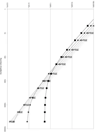
Figure 4.1 shows the break even point for range look-ups (l) given a

number of call-sites and patterns. As the break even point is in percentages all cases bigger than 100% mean that the 2-order B+-tree implementation would be more expensive than a hash table. Figure 4.1 shows that when applying one or two patterns the hash table is always the fastest solution. The more patterns are applied the lower the break even point becomes. What is notable is that with an increasing number of patterns all break even points eventually level out. This can be seen by the “500 call-sites”

case that levels out around 0.53% but is also visible in the figure for the

5000 and 50 000 cases.

(25)

1 1 0 1 0 0 1 0 0 0 1 0 0 0 0 1 0 0 0 0 0 0 .0 1 % 0 .1 0 % 1 .0 0 % 1 0 .0 0% 1 0 0 .0 0 % 5 0 0 5 k 5 0 k 5 0 0 k 5 M 5 0 M 5 0 0 M N u m b e r o f p a tte rn s

[image:25.595.167.482.143.579.2]

Break even point hash and 2-order B+-tree in percentage

Figure 4.1: Break even point for range look-ups (l) for hash and 2-order

B+-tree by number of call-sites and patterns. If for a given number of

(26)

[image:26.595.110.449.126.644.2]

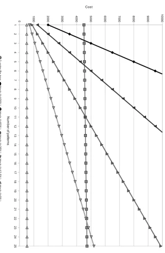
4.1. Indices 1 2 3 4 5 6 7 8 9 1 0 1 1 1 2 1 3 1 4 1 5 1 6 1 7 1 8 1 9 2 0 2 1 2 2 2 3 2 4 2 5 0 1 0 0 0 2 0 0 0 3 0 0 0 4 0 0 0 5 0 0 0 6 0 0 0 7 0 0 0 8 0 0 0 9 0 0 0 1 0 0 0 0 2 -o rd e r B + -tr e e H a s h (l= 1 0 0 % ) H a s h (l= 5 0 % ) H a s h (l= 2 5 % ) H a s h (l= 1 2 .5 % ) H a s h (l= 0 % ) N u m b e r o f p a tte rn s Cost

Figure 4.2: Comparison of cost for applying a number of patterns for the

(27)

such as Subversion, 5 million lines of code represent suites such as OpenOffice whereas 50 to 500 million lines of code represents main stream operating systems and distributions such as Windows and Debian [1].

Figure 4.2 shows the influence of the percentage of range look-ups in case of 500 call-sites. As the percentage of range look-ups does not matter for a B+-tree there is only one data set for B+-trees and a number of hash data

sets for different range look-up percentages (l). What clearly shows is the

bigger initial cost for setting up the B+-tree, roughly 9 (log2(500)) times

higher than for the hash table.

This figure can be compared with a small part of Figure 4.1. Both

figures show that for one or two patterns hashes are faster regardless of the percentage of range look-ups and that the higher the number of patterns becomes, the lower the percentage of range look-ups becomes for which a hash table is faster than a B+-tree.

It can be concluded that different indexing mechanisms have different characteristics and that determining which mechanism to use must be a run-time decision. This means that the complexity considerations must be done at run-time, making it both more complex and flexible.

4.2

Selectivity

The principle behind selectivity is that the most efficient way to search a single table is determined. This is done by determining how complex, computational-wise, the different selections are. A selection is a filter that

selects a subset of the whole table or theWHEREclause of SQL statements.

This section assumes a table “call sites” that contains all call-sites, sim-ilar to Table 2.2, instead of the design described in Chapter 3.

4.2.1 Theory

The primary look-up is from pattern to call-sites and not the other way around. The call-sites are stored in a (single) table which is scanned, i.e. there is no need for optimising the aggregation of data from multiple tables. There are (database) normalisations that would make the storage of call-site signatures spread over multiple tables, but those would not be much more than a table of types which are then linked to the call-sites table by means of a foreign key which is usually associated with an index. For the reverse look-up, i.e. from call-site to patterns, there seems to be use for a join optimiser as there are (conceptually) several classes of sub-patterns that can be queried independently.

However, the pattern to call-sites look-up is no more than doing a se-lection on the call-sites table, like in Listing 4.1 which is a pattern that

matches allintwith GetCapacityas name. This is where statistics about

(28)

4.2. Selectivity

S E L E C T *

F R O M c a l l _ s i t e s W H E R E

r e t u r n _ t y p e = ’ int ’ AND n a m e = ’ G e t C a p a c i t y ’

Listing 4.1: Example SQL query for pattern

used to estimate the “selectivity factor” (F) for each of the predicates of the

WHEREclause of a SQL statement [22]. TheF for a predicate is determined based on the estimated uniqueness of the value in the table.

This uniqueness can already be known because of the creation of his-tograms which were needed for indices. Otherwise, one has to use another heuristic. For such a heuristic a study of the actual call-sites in an applica-tion needs to be performed.

A simple heuristic would be to determine the average number of call-sites per generic-functions, but this assumes that they are evenly spread which might not be the case.

The following gives the selectivity factors for different kinds of

predi-cates [22]. The selectivity factor (F) is in this case a number between 0 and

1. These selectivity factors are all independent best-guess values.

Exact pattern : pred= “GetN ame00

F(pred) = #Occurrences(“GetN ame00)/#call sites

F(pred) = 1/#generic f unctions

As can be seen there are two approaches to calculate the selectivity a pattern. The first one is when one has information about how often the pattern occurs, i.e. a histogram, whereas the latter has no specific information.

Wild card pattern : pred= “Get∗00

F(pred) = #Occurrences(“Get∗00)/#generic f unctions

A wild card pattern is much trickier; a full wild card matches every-thing and thus has a selectivity of 1. However, for partial wild card patterns, like “Get*”, one needs to know how often it occurs or make an educated guess based on the content of the non-wild card part of the pattern. The educated guess needs research into how function names are generally constructed and thus how unique the non-wild card part will roughly be. See Chapter 5 for more information.

Inverse predicate : pred=!(pred0)

F(pred) = 1−F(pred0)

(29)

Conjunction of predicates : pred=pred0 and pred00:

F(pred) =F(pred0)×F(pred00)

Under the assumption that the predicates are independent, the chance of row in the set matching pred’ to exist in the set matching pred” is as big as the chance of a random row existing in the set of matching pred”s. As such their selectivity factors can be multiplied.

Disjunction of predicates : pred=pred0 or pred00

F(pred) =F(pred0) +F(pred00)−F(pred0)×F(pred00)

For the or predicates we can sum the factor of both predicates and then exclude the intersection of the rows matching both predicates, i.e. subtract the selectivity factor of the conjunction of pred’ and pred”.

The selectivity factor makes assumptions about even distribution and independency between predicates. With applications this will generally not be the case; some generic-functions will be referenced much more often than others. Therefore optimisation based on selectivity factors can actually be (way) worse than the best optimisation. However, getting the exact selec-tivity factors means doing the actual selection which is the thing we want to optimise, not execute more often.

4.2.2 Application of theory

Given Listing 4.1, what would be the selectivity? The first step is figuring out what the selectivity of the different parts of the predicate. First the

return_type = ’int’; this is an exact pattern, however it occurs 5 times

in the 15 call-sites of Table 2.2. This means thatF = 5/15 = 0.33. When

there is no histogram of the occurrences, it is impossible to tell it occurs 5 times and one has to estimate. The generic-functions have four different

return-types, so given the mean that would result in a F = 4/15 = 0.27.

The median amount of call-sites per return-type is 3.5, resulting in aF =

3.5/15 = 0.23.

The next step is determiningname = ’GetCapacity’’s selectivity factor.

It occurs one time in the 15 call-sites giving it aF = 1/15 = 0.07. There are

5 different names, giving aF = 3/15 = 0.2 (the mean) which overestimates

the real number by a factor 3.

The final step is determining the AND’s selectivity factor. This is simply

F = 0.33×0.07 = 0.02, however with the estimations this would become

F = 0.27×0.2 = 0.06 which is closer to the actual selectivity ofF = 1/15 =

0.07 than the version without estimates because thereturn_type = ’int’

does not add any restrictions oncename = ’GetCapacity’ is evaluated.

When looking at wild card patterns, e.g.name = ’Get*’, the selectivity

(30)

4.3. Query reordering

Name Occurrences

Get... 8

wai... 4

Cha... 2

[image:30.595.218.328.127.206.2]

Aft... 1

Table 4.3: Histogram of first three letters of name from the generic-function call-sites in the snippets from Listing 2.1.

the pattern matches 8 in 15, orF = 0.53, of the generic-function call-sites,

however the mean and median would be respectively 3.75 and 3.

This means that there is possibly a need for histograms, but the real

question is how much better do histograms make the estimations? and how

much does making and querying histograms cost?. This requires extra study-ing, but falls outside the scope of this research as more empirical information is needed.

4.3

Query reordering

The principle behind query reordering is that an order of the individual parts of the query is determined to yield the minimum amount of processing required. This is done by determining how complex, computational wise, the individual parts are as well as the size of the resulting search space. The reordering results in a “search-plan”.

This section assumes the design described in Chapter 3, however the theoretical explanation uses a different example as the design from Chapter 3 makes the example unnecessarily complex.

4.3.1 Theory

The major problem with determining the best order is that there are many different orders and that the computational complexity and resulting search

space of the individual parts (n), e.g. sub-patterns, depends on the already

executed parts, basically meaning that there are in worst case n! different

orderings [3, 15].

However, the search space for the best search-plan can be drastically reduced. For example when getting information from multiple tables by making sure that the intermediate results stay relatively small. For example imagine the SQL query in Listing 4.2 and the data as given in Table 4.4. In

this examplea.ssnis a unique key, i.e. the values are unique and there is a

(31)

S E L E C T b . n a m e

F R O M a J O I N b ON a . id = b . id

W H E R E a . ssn = ’ 1 2 3 4 ’ AND b . g e n d e r = ’ m a l e ’

Listing 4.2: Initial SQL query

a.ID a.SSN

1 2341

2 1234

3 3412

4 4123

b.ID b.Name b.Gender

1 Jane Female

2 John Male

3 Pete Male

4 Penny Female

Table 4.4: Example tables for Listing 4.2.

Table 4.5 shows what happens when first the Cartesian product of the two tables is calculated before continuing with filtering that data. In total the table would be 16 records long, the product of the size of both table a and table b.

a.ID a.SSN b.ID b.Name b.Gender

1 2341 1 Jane Female

1 2341 2 John Male

1 2341 3 Pete Male

1 2341 4 Penny Female

.. .. .. .. ..

Table 4.5: Example of the Cartesian product of Table 4.4.

When first getting the record fromawithssn = ’1234’as intermediate

result the Cartesian product would be significantly smaller as there can at

most one record in a with that ssn due to the unique key. The resulting

Cartesian product can be seen in Table 4.6. When taking indices into ac-count one can optimise the scanning of the tables away, but this is explained in Section 4.1. In these examples it is assumed that half of the people is male.

The search space for the search-plan is reduced in three steps. First the ‘query tree’, i.e. the tree representation of the initial query, is simplified into a “master plan”. The master plan groups consecutive commutative and

as-sociative operators of the same kind. For example(a JOIN b) JOIN cand

a JOIN (b JOIN c)are equivalent and can be stored as oneJOINoperation in the master plan.

(32)

mas-4.3. Query reordering

a.ID a.SSN b.ID b.Name b.Gender

2 1234 2 John Male

2 1234 3 Pete Male

2 1234 4 Penny Female

Table 4.6: Example of the Cartesian product of Table 4.4 using a reduced

intermediate result for a.

ter plan. At this stage the “selections”, e.g. a.ssn = ’1234’ are pushed

down in the ’query tree’. For example Listing 4.2 would be transformed into Listing 4.3. The rationale behind this step is that reducing intermediate re-sults speeds up execution, although there are cases where not fully pushing down the selections results in a faster execution. For example when joining two tables an index on the “join selection” means faster look-up of records in the joined table. What would happen to the example tables can be seen in Table 4.7.

S E L E C T d . n a m e F R O M (

S E L E C T a . id F R O M a

W H E R E a . ssn = ’ 1 2 3 4 ’ ) AS c J O I N (

S E L E C T b . id , b . n a m e F R O M b

W H E R E b . g e n d e r = ’ m a l e ’ ) AS d ON c . id = d . id

Listing 4.3: SQL query with fully pushed selections

a.ID a.SSN

2 1234

b.ID b.Name b.Gender

2 John Male

3 Pete Male

Table 4.7: Example tables for pushed down selections.

Doing the (pushed) selection before the join might remove this index and just make the actual joining slower. An example of this is Listing 4.3 which would be slower to execute than Listing 4.4 when there is an index on

b.idbecause the intermediate resultscand ddo not have an index. In the

(33)

2 records, or half of b. On the join the whole reduced b would need to be

iterated, but what is worse is that there is no index onb.gender causing,

in effect, the whole ofbto be iterated to get the intermediate set.

With the partial push, visualised in Listing 4.4, the join would use the

index onb.idand do a join with only one record in the table followed by the

b.gender = ’male’ selection. Because of this several plans are generated with different levels of pushed down selections.

S E L E C T b . n a m e F R O M (

S E L E C T a . id F R O M a

W H E R E a . ssn = ’ 1 2 3 4 ’

) AS c J O I N b ON c . id = b . id W H E R E b . g e n d e r = ’ m a l e ’

Listing 4.4: SQL query with partially pushed selections

The third step simplifies the “logical query execution plans” into ‘left-deep query trees’ which are the final output of the reordering. A left-‘left-deep query tree is a binary tree of joins where the right node is always a leaf node containing a single operation to do. Operations in this case would be selections and joins. The advantage of such a tree is that implementing “pipe-lining” is possible. With pipe-lining the results of a join are piped into the next join which means that there is no need to store intermediate results. The most important benefit is that this reduces the join search

space (joiningntables) fromO(n!) toO(2n) [14].

To create an optimal left-deep tree all permutations of the joins must be considered. As this number of permutation grows exponentially some heuristics must be used to cut corners to create a good, although not neces-sarily the best, query plan quickly. One of the methods that can be used is dynamic programming as described by [22]. This method works as follows: first several “1-relation plans” are made, at least one per tuple of to-be-joined tables although there can be more depending on existing indices. These plans are then evaluated, i.e. a value is given to the plan based on their estimated execution cost. Then the best of these plans are chosen to be joined with another table, i.e. a tuple for each chosen 1-relation plan with a table that is not in the plan. This results in several “2-relation plans” that

are evaluated and the cycle continues until then-relation plan has expanded

to contain all tables. This n-relation plan is the result, i.e. search-plan, of

(34)

4.4. Summary

4.4

Summary

With query reordering all of the theory from this Chapter comes together. The existence and type of indices have great influence on the cost of exe-cution, whereas the selectivity factor tells what might be the better way to reduce the size of the intermediate data and then the query reordering helps us to decide how to order the query to quickly determine a good plan for executing the query.

The following example will show how all the theory can be applied. In the example pattern 2 from Table 2.1 will be matched against the call-sites. The first step is determining the selectivity of the different components of the pattern that needs to be matched. The number of occurrences and their selectivity can be seen in Table 4.8.

Sub-pattern To

matc

h

Occurrences Selectivit

y

Index Lo

ok-up

cost

Cost

es

tim

at

e

Kind call 11 0.73 Hash O(1) 12

Modifiers public 11 0.73 B+-tree O(log n) 15

Type Cargo 3 0.20 Hash O(1) 4

Class * 15 1.00 Hash O(3n) 35

Name Get* 8 0.53 B+-tree O(log n) 12

Parameters - 12 0.80 None O(n) 15

Table 4.8: The selectivity information for pattern 2 and the used index per sub-pattern.

The table clearly shows that the class sub-pattern selects everything and as such is not useful for the result and that selecting on Cargo is the most selective. However, the selectivity is not what the focus should be on, but the expected cost which is shown in the last column. This cost is the sum of the look-up cost and the cost for looping through linked lists and/or range look-up, i.e. the number of occurrences. The expected costs are important because doing a slightly less selective range look-up on a B+-tree indexed variable is faster than doing a range look-up on a hash table indexed variable. In the former case one would only need to scan the resulting, usually significantly smaller, sub set on the most selective variable which means doing less comparisons in total.

(35)

round that adds another sub-pattern until all sub-patterns of the pattern are in the order.

When applying the methods from query reordering, the best or most promising options are chosen. In this case the type sub-pattern is most selective, i.e. should be evaluated first. The kind pattern and name pattern are equally promising so both go to the next round.

In this second round a design difference between the modeling of the data in databases and Java will be encountered. In databases each table is linked to another by means of an identifier, which is usually indexed. However, in Java connections are made by means of references. This means that the joins in Java are essentially free, i.e. one just needs to loop over the intermediate result set and query the sub elements directly. This means that reducing the result set becomes most important, i.e. using the selectivity factors.

First pattern Second pattern Estimated. sel. Actual. sel Cost

Type Base 0.15 0.20 6

Type Modifiers 0.15 0.20 6

Type Name 0.11 0.20 6

Type Parameters 0.16 0.20 6

Base Modifiers 0.53 0.73 20

Base Type 0.15 0.20 14

Base Name 0.39 0.53 18

Base Parameters 0.58 0.53 21

Name Base 0.39 0.53 18

Name Modifiers 0.39 0.53 18

Name Type 0.11 0.20 14

Name Parameters 0.42 0.53 18

Table 4.9: The selectivity information for pattern 2 and the used index per sub-pattern.

(36)

4.5. Conclusion

many comparisons were done to get the first intermediate result, plus the size of the expected result set, i.e. the size of the second intermediate result. It has to be noted that after the first round the histogram data becomes unreliable because there are usually correlations between sub-patterns. For example the name pattern “Get*” and its return type non-void. Thus when the “Get*” pattern is matched matching the return type for being non-void is a waste of time. However, making the query optimizer aware of that fact in a generic manner is far from trivial. Especially as it is unknown what dependencies between sub-patterns or parts of a signature exist.

4.5

Conclusion

Three major facets from the database field have been studied: indexing data sets, determining selectivity of a sub-pattern, i.e. how many results will matching a sub-pattern give, and query reordering, i.e. ordering the sub-pattern matches in the most effective way. All these facets can be used to improve the performance of matching call-sites to patterns and vice versa. However, the “join” optimisation of the latter method will not be needed.

Determining selectivity of a sub-pattern can be used to quickly reduce the result set and thus reduce the number of evaluations, however it still requires a full scan of the table when there is no index. As such selectiv-ity measurements can only reduce the number of sub-pattern matches to determine whether a particular pattern matches; it cannot skip patterns completely when it is known they cannot match. However, as it is possible to determine what index is best at run-time, the most selective sub-pattern is a good, if not the best, candidate to add the index to.

Having indices on certain sub-patterns can be used to get a small sub set of the initial data set by partly removing the need to scan the data set. However, there are different indexing methods that have their own characteristics. A (sorted) B+-tree can quickly scan a range of the data set due to logarithmic access, however the costs for creating and maintaining a B+-tree are high. A hash table has an extremely fast look-up for a specific value, but for a range look-up a full scan of the table is needed. As a hash table is bigger than an the actual data set, such range look-ups are more costly than in an unsorted unindexed array.

(37)

selective sub-pattern that has mostly exact look-ups and thus can use hash look-ups. This will decrease the performance of the look-ups slightly, but an application will most likely not keep loading specialisations, thus patterns, or classes, thus call-sites, infinitely and therefore the extra look-up costs can dwarf the cost for building the B+-tree.

(38)

Chapter 5

Call-site and pattern survey

In the previous chapter we have presented indices and search-plan optimiza-tion as possible optimizaoptimiza-tions for pattern evaluaoptimiza-tions. In order to apply these mechanisms some knowledge about the structure of the data on which queries are performed is needed. For instance, it must be known for which sections of signatures the effort of keeping an index may pay off; for search-plan optimization, heuristics are needed to estimate the selectivity of certain sub-patterns.

In this chapter a survey of real-world applications and aspects is done to be able to answer what the best strategy for optimizing pattern to call-site look-up is. To answer this question the following sub problems have to be

addressed first: what are the general characteristics of call-sites and

generic-functions in real world applications? andwhat are the general characteristics of patterns in real world aspects?.

These sub problems are solved in respectively Section 5.1 and Section 5.2. Finally Section 5.3 formulates optimization strategies based on the findings of both sections.

5.1

Call-site characteristics

(39)

5.1.1 Methodology

To acquire the call-site information a small tool, called Extract, has been written to extract the call-site information from Java class files. Extract uses ASM [8], a Java byte code framework, to read the Java class files and parts of the SiRIn core, a reference implementation of ALIA4J, to determine what generic-function a call-site belongs to.

The input to Extract is a list of Java class files or Java archives with Java class files of a particular application. All Java class files and all classes they reference are analysed recursively. Examples of referenced classes are the super class, classes used as return or parameter type, classes of instance variables and classes used in the implementation of a method. The final result of Extract is a list with all generic-functions and the number of times they were referenced.

The recursive behaviour of the analysis means that a large part of the Java API’s implementation will be part of the output. However, the imple-mentation of the Java API should be seen as a black box and one would generally not want to add aspects that modify the API’s implementation. AspectJ, e.g. thus applies aspects only to the files that it compiles itself; this excludes the class files of the Java API. These internal calls are there-fore ignored by this survey. Nevertheless, calls to the Java API from the application are of importance. After the extraction the data is analysed using common data mining techniques to find correlations and significant information.

The applications that have been analysed in this context are the following four:

• ANTLRA tool to construct parsers, compilers and translators.

• FreeColA turn-based strategy game.

• LIAMA major part of the implementation of ALIA4J.

• TightVNCAn application to remotely take over a desktop.

These applications are varied in nature in an attempt to get a general view of the call-site characteristics instead of only getting a view of non-graphical applications that do not use a network connection, as is commonly the case for benchmark suites used in performance evaluation [5].

(40)

5.1. Call-site characteristics

5.1.2 Acquired information

Statistics The analysed applications have 2 432 classes containing a total of 28 065 generic-functions and 150 432 call-sites. The following sections will discuss the most salient features separately for each generic-function kind; only the breakdown on class names is presented in a single section as it is almost the same in all cases.

Storage Per generic-function kind there is also a discussion on the best storage technique for quickly retrieving call-sites per sub-pattern kind on the basis of the information gathered. The techniques considered here are “bucket arrays”, like hash tables, and “sorted collections”, like B+-trees.

Section 5.1.8 summarises with a comparison of the storage techniques over the different sub-patterns looking at differences and similarities in the use of patterns between the different sub-patterns.

5.1.3 Class names

Statistics The combined test input consists of 2 432 different classes that

are spread over 147 packages, on average placing roughly 16.5 classes in each

package.

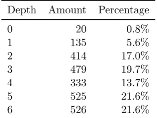
Depth Amount Percentage

0 20 0.8%

1 135 5.6%

2 414 17.0%

3 479 19.7%

4 333 13.7%

5 525 21.6%

[image:40.595.194.353.418.537.2]

6 526 21.6%

Table 5.1: Package depth for class names

Table 5.1 shows the classes’ package depth, i.e. the number of super packages a class has before reaching the “unnamed” default package. The 20 classes with depth 0, i.e. the ones placed in the unnamed package, and 135 classes with depth 1 do not comply with the standard practice of using a reverse DNS name. The classes at depth 2 are primarily from the Java API, whereas classes at depths of 4 and more are almost exclusively used by applications.

(41)

of checks: Assume the classes of the Java API are lexically sorted by their fully qualified name and are put in a sorted set. Then all classes that match thejava.lang..*pattern can be found by calculating a subset: the starting

point of the range is constructed by removing.*from the pattern, the end

point is constructed by replacing ..* with / (U+002F), whose codepoint

the Unicode character encoding places immediately after the . (U+002E).

Calculating the subset only requires two O(log n) comparisons. When a

pattern starts with.*then the whole sorted set is returned.

Storage When looking at the storage techniques the first option is using a sorted collection. This has the benefit of ordering all classes lexically by name; thus the aforementioned technique can be used. However, storing all classes into buckets by package can be used to efficiently look up all classes in a given package, but due to the use of sub-packages one has to determine how to find all classes that are in a particular package or sub-package. Either the buckets also contain references to sub-packages which are then recursively searched or each class gets inserted into its package and all ancestor packages. A major drawback of the latter technique is the fact that the number of times the class is referenced is equivalent to the package depth plus one. The former technique resembles the behaviour of a sorted collection.

5.1.4 Static initialisers

Statistics A total of 571 static initialiser were found. The static initialisers do not have a call-site, i.e. they are called implicitly, and the name, modi-fiers, return type, parameters, and exceptions are the same for every static initialiser. As such the only way to distinguish between static initialisers is their containing class which means there is at most one per class.

Furthermore none of the static initialisers are of the Java API and as

such there are no class names starting withjava.

Storage Static initializers only have one sub-pattern: the declaring-class pattern. Thus, the same considerations as in Section 5.1.3 apply.

5.1.5 Constructors

Statistics A total of 3 034 constructors were found; on average about 1.25 constructors have been found per class.

(42)

Modifier Amount Percentage

package visible 759 25.0%

public 1 971 65.0%

private 151 5.0%

protected 153 5.0%

transient 14 0.5%

annotation 53 1.7%

[image:42.595.175.373.129.252.2]

deprecated 7 0.2%

Table 5.2: Modifier usage for constructors

# Parameters Amount Percentage

0 669 22.1%

1 1 171 38.6%

2 720 23.7%

3 241 7.9%

4 144 4.7%

[image:42.595.177.371.297.403.2]

5+ 89 2.9%

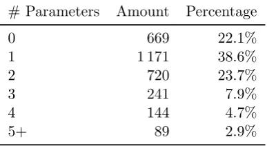
Table 5.3: Parameter usage for constructors

Table 5.3 relates the number of parameters to the amount of constructors having such a parameter count. The 3 034 constructors declare a total of

4 420 parameters, giving about 1.5 parameters per constructor. Of all these

parameters 588 are of type java.lang.String, 564 are int and 158 are

boolean, from a total of 518 parameters types.

Of the 3 034 constructors 2 855 do not throw an exception, leaving 179 that do throw at least one. A total of 188 exceptions is declared; a few constructors declare more than one exception. The exceptions most

fre-quently thrown arejavax.xml.stream.XMLSteamException(84 times) and

java.io.IOException (40 times), which are both part of the Java API.

A total of 14 526 call-sites of constructors were found. Of these 64% call a constructor from the Java API; only 36% of the calls are for creating

appli-cation specific classes. Classes from thejava.lang package are constructed

39% of the time, with theStringBuffer/StringBuilderbeing responsible

for over 50% of the calls. Most of these string building calls are generated au-tomatically by the compiler when it encounters the concatenation of strings

using the+ operator. This means that in theory these call-sites should not

(43)

Storage The name of a constructor can be best stored in a sorted col-lection as it is similar to the class names; it has many unique names as well.

For the modifiers a bucket array is best as there are only a few valid different buckets to consider. However, there are sometimes multiple buckets a constructor would match with. In that case they have to be put in all, but this is not a big problem as a relatively small amount would be placed in multiple buckets. It has to be considered whether physically storing the

publicmodifiers bucket is needed at all, as it matches the vast majority of constructors.

We consider three techniques to store parameters: First, the number of parameters can be used to determine the bucket. Second, the first parameter

type can be used. (If a function has no parameters, void is used as first

parameter.) Third, the concatenation of all parameter-type names can be stored lexically sorted.

The benefit of the first technique is that searching for a particular amount of parameters is extremely efficient, whereas the second is efficient in finding constructors that have a particular type as first parameter.

The third technique is well suited for finding constructors that start with particular parameters, but finding constructors with a given length requires looking through the whole collection.

Finally the exceptions can best be stored in a bucket as well. Here, each declared exception is put into a bucket. Given the low amount of actually declared exceptions and the low amount of constructors with more than one declared exception this does not impact storage much. The constructors that do not throw an exception are not stored specially.

5.1.6 Field reads and writes

Statistics In total, 3 884 fields have been found, yielding 1.6 fields per class. Of these fields 3 874 are read and 3 863 are written. Some fields,

pri-marily with aprotectedaccess modifier, are not written to or not read. As

these fields are all part of the Java API this can be explained by the appli-cation extending such a framework class and only then writing or reading said fields.

An example of this can be seen withjavax.swing.JComponent.ui. This

field of JComponent has a protected access modifier and a method to set

it. It does not have a function to read the value, though. Thus if a custom,

non Java API, sub lass ofJComponent requires information from that field

it needs to access it directly. As a result there is a field read on that field, but the application does not (directly) write to it, so there is no field write. All static final reads are ignored because the majority of call-sites can be silently destroyed by the compiler optimising them away.

(44)

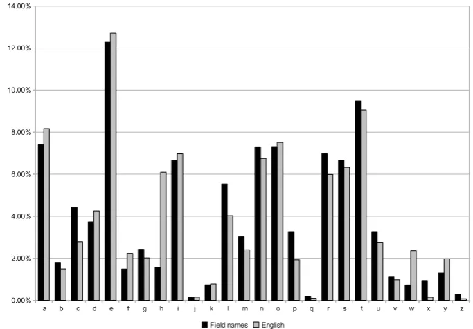
field nameloggeris used 38 times which means that the field names

them-selves are all quite selective. The majority, 95.9%, of the field names start

with a lower case letter. Of the 3.2% of field names that start with an upper

case letter 55.6% are static. About 0.9% of all names start with either a

$(U+0024) or a _(U+005F).

The field names have an average length of 9.7 characters. Around 99%

of these characters are letters. Looking at the first three characters does

not show any discernible patterns; the most prefix, can, is used in less than

1.75% of the field names. This means that the field names diverge relatively

fast in all cases.

The length and divergence of the field names can be used to estimate

the time required for one comparison of two strings. If, e.g., at most 1.75%

of the field names start with the same three letters one knows that in three

comparisons there is at most a 1.75% chance that further characters have

to be examined.

71 $

52 0 25 1 26 2 2 3 11 4 10 5 1 6 1 7 8 8

241 _

Field names English

2759 a 7.40% 8.17% 1.104187872 0.905642984 0.905642984 0.09 671 b 1.80% 1.49% 0.829427481 1.205650913 0.829427481 0.17 1645 c 4.41% 2.78% 0.630845982 1.585172972 0.630845982 0.37 1391 d 3.73% 4.25% 1.140513343 0.87679816 0.87679816 0.12 4578 e 12.27% 12.70% 1.034971612 0.966210076 0.966210076 0.03 556 f 1.49% 2.23% 1.494763597 0.66900211 0.66900211 0.33 906 g 2.43% 2.02% 0.829619536 1.205371807 0.829619536 0.17 588 h 1.58% 6.09% 3.86595898 0.258668032 0.258668032 0.74 2477 6.64% 6.97% 1.049034041 0.953257912 0.953257912 0.05 51 0.14% 0.15% 1.11906 0.893607135 0.893607135 0.11 274 k 0.73% 0.77% 1.050990657 0.951483244 0.951483244 0.05 2064 l 5.53% 4.03% 0.727425145 1.374711895 0.727425145 0.27 1127 3.02% 2.41% 0.796349707 1.255729726 0.796349707 0.20 2724 n 7.30% 6.75% 0.924196762 1.08202067 0.924196762 0.08 2727 7.31% 7.51% 1.026865105 0.973837747 0.973837747 0.03 1220 p 3.27% 1.93% 0.589799656 1.695490986 0.589799656 0.41 74 q 0.20% 0.10% 0.478877027 2.088218778 0.478877027 0.52 2599 r 6.97% 5.99% 0.859280777 1.16376396 0.859280777 0.14 2486 s 6.66% 6.33% 0.949355406 1.053346295 0.949355406 0.05 3537 t 9.48% 9.06% 0.955066192 1.047047847 0.955066192 0.04 1220 3.27% 2.76% 0.843269803 1.185860084 0.843269803 0.16 413 v 1.11% 0.98% 0.883325811 1.132085112 0.883325811 0.12 272 0.73% 2.36% 3.236497059 0.308976026 0.308976026 0.69 351 x 0.94% 0.15% 0.159410256 6.273122085 0.159410256 0.84 484 y 1.30% 1.97% 1.521366694 0.657303728 0.657303728 0.34 108 z 0.29% 0.07% 0.255587778 3.912550157 0.255587778 0.74

i j m o u w

a b c d e f g h i j k l m n o p q r s t u v w x y z 0.00% 2.00% 4.00% 6.00% 8.00% 10.00% 12.00% 14.00%

[image:44.595.96.438.340.578.2]

Field names English

Figure 5.1: Letter frequencies of field names compared to English

Figure 5.1 shows the letter frequencies in the field names which are fairly similar to the letter frequencies in English, although there are a few letters whose frequency differs significantly.

(45)

public 236 6.1%

private 2 189 56.4%

protected 597 15.4%

static 395 10.2%

volatile 8 0.2%

transient 50 1.3%

annotation 22 0.6%

[image:45.595.221.419.128.280.2]

deprecated 9 0.2%

Table 5.4: Modifier usage for fields

more oftenprivatethan constructors are. This situation is reversed for for

public.

public 52 13.2%

private 291 73.7%

protected 12 3.0%

volatile 3 0.8%

[image:45.595.222.421.371.483.2]

annotation 22 5.6%

Table 5.5: Modifier usage for staticfields

Table 5.5 shows the modifiers, but only for the static fields. What

stands out is that all package visible fields are also static and that there

are much fewerprotected fields and fields without modifiers than for

non-staticfields.

For field writes the (hypothetical) return type is always void whereas

for field reads there is no parameter type. As the return type of a field read is the same as the parameter type of a field write for the same field, these types are the same. Of these types 53% is either a primitive or comes from thejava.lang package, with int,boolean and java.lang.String taking respectively 22%, 12% and 10% of the total.

Field reads and writes cannot throw checked exceptions.

A total of 27 979 field reads and 9 752 field writes, respectively 7.2 and

2.5 per field. Roughly 16.4% are reads from and 12.4% are writes to classes

(46)

Storage For storing the name a sorted collection makes finding a partic-ular name or a range easy. Using a bucket array is possible, but either the whole name has to be hashed or only the first character is taken into ac-count. In the former case doing a name range look-up becomes expensive, whereas in the latter case one still has to go through a long list of items after the first bucket. If one were to chain the buckets per character one would in effect be building sorted collection.

The modifiers can only be stored in a bucket array due to the limited amount of options. It can be considered to not create a physical bucket for the private fields as they match more than half of the fields and as such are not very selective.

The type of the field can best be stored in a sorted collection. There are quite a number of types, although it is very conceivable that a set of types from one package is considered. In that case having a collection sorted on the type name would make getting those ranges work in the same way as for class names. However, it is conceivable to store the data in a bucket array if there can be, e.g. due to a less powerful point cut languages, are no range look-ups on the type of a field.

5.1.7 Methods

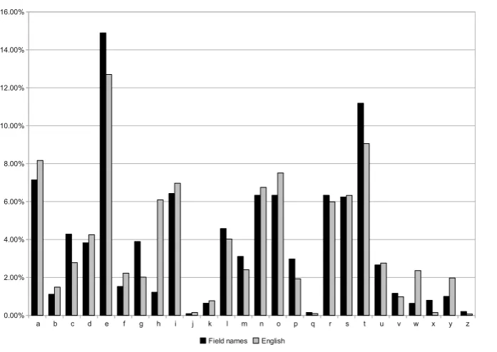
Statistics A total of 17 294 methods were found, which means about 7.1 methods have been found per class. There are 6 812 different names for the

methods, yielding 2.5 methods with the same name.

The average length of a method name is 12.3 characters; almost 3

char-acters more than field names. Around 99% of the charchar-acters are a letter. Figure 5.2 shows the letter frequency in the method names which is less similar to the letter frequency in English. Letters “c”, “e”, and “t” are used significantly more often whereas the usage of letters such as “h”, “w”, and “y” have dropped by up to 75%.

Name Amount Percentage

get 4 596 25.6%

set 1 346 7.8%

cre 541 3.1%

acc 499 2.9%

add 413 2.4%

Table 5.6: Frequency of first three letters in method name

(47)

459 $ 895 0 199 1 185 2 92 3 86 4 57 5 50 6 39 7 46 8 24 9

513 _ Field names English

15203 a 7.15% 8.17% 1.142960987 0.874920502 0.874920502 0.13 2370 b 1.11% 1.49% 1.339425688 0.746588638 0.746588638 0.25 9108 c 4.28% 2.78% 0.649878621 1.53874888 0.649878621 0.35 8136 d 3.82% 4.25% 1.112199228 0.899119488 0.899119488 0.10 31686 e 14.89% 12.70% 0.852909275 1.172457645 0.852909275 0.15 3247 f 1.53% 2.23% 1.459926677 0.684965907 0.684965907 0.32 8285 g 3.89% 2.02% 0.517464647 1.932499169 0.517464647 0.48 2599 h 1.22% 6.09% 4.988779592 0.200449826 0.200449826 0.80 13677 6.43% 6.97% 1.083654328 0.922803494 0.922803494 0.08 196 0.09% 0.15% 1.660861837 0.602097043 0.602097043 0.40 1358 k 0.64% 0.77% 1.209527305 0.826769264 0.826769264 0.17 9735 l 4.58% 4.03% 0.8796868 1.136768222 0.8796868 0.12 6612 3.11% 2.41% 0.774213829 1.291632831 0.774213829 0.23 13478 n 6.33% 6.75% 1.065398602 0.938615836 0.938615836 0.06 13474 6.33% 7.51% 1.185408452 0.843591083 0.843591083 0.16 6333 p 2.98% 1.93% 0.64806846 1.543046855 0.64806846 0.35 324 q 0.15% 0.10% 0.623845062 1.602962116 0.623845062 0.38 13476 r 6.33% 5.99% 0.945249383 1.057921876 0.945249383 0.05 13281 s 6.24% 6.33% 1.013596738 0.986585653 0.986585653 0.01 23797 t 11.18% 9.06% 0.80967802 1.235058845 0.80967802 0.19 5658 2.66% 2.76% 1.037121089 0.964207565 0.964207565 0.04 2472 v 1.16% 0.98% 0.841760485 1.18798639 0.841760485 0.16 1347 0.63% 2.36% 3.727713734 0.268260943 0.268260943 0.73 1697 x 0.80% 0.15% 0.18806482 5.317315586 0.18806482 0.81 2132 y 1.00% 1.97% 1.969963114 0.507623718 0.507623718 0.49 438 z 0.21% 0.07% 0.359464292 2.781917486 0.359464292 0.64

i j m o u w

a b c d e f g h i j k l m n o p q r s t u v w x y z 0.00% 2.00% 4.00% 6.00% 8.00% 10.00% 12.00% 14.00% 16.00%

[image:47.595.149.498.125.372.2]

Field names English

Figure 5.2: Letter frequencies of method names against English

areaccess$nmethods created by the compiler for inner classes that try to access outer classes.

Table 5.7 shows how often a particular modifier is used for a method. As multiple modifiers can be used at the