Efficient algorithms for local forest similarity and forest pattern matching

(1)

Scholarship@Western

Electronic Thesis and Dissertation Repository

7-21-2014 12:00 AM

Efficient algorithms for local forest similarity and forest pattern

matching

Fang Han

The University of Western Ontario Supervisor

Kaizhong Zhang

The University of Western Ontario

Graduate Program in Computer Science

A thesis submitted in partial fulfillment of the requirements for the degree in Master of Science © Fang Han 2014

Follow this and additional works at: https://ir.lib.uwo.ca/etd Part of the Bioinformatics Commons

Recommended Citation Recommended Citation

Han, Fang, "Efficient algorithms for local forest similarity and forest pattern matching" (2014). Electronic Thesis and Dissertation Repository. 2182.

https://ir.lib.uwo.ca/etd/2182

This Dissertation/Thesis is brought to you for free and open access by Scholarship@Western. It has been accepted for inclusion in Electronic Thesis and Dissertation Repository by an authorized administrator of

(2)

EFFICIENT ALGORITHMS FOR LOCAL FOREST SIMILARITY

AND FOREST PATTERN MATCHING

(Thesis format: Monograph)

by

Fang Han

Graduate Program in Computer Science

A thesis submitted in partial fulfillment

of the requirements for the degree of

Masters of Science

The School of Graduate and Postdoctoral Studies

The University of Western Ontario

London, Ontario, Canada

c

Fang Han 2014

(3)

Ordered labelled trees are trees where each node has a label and the left-to-right

order among siblings is significant. Ordered labelled forests are sequences of ordered

labelled trees. Ordered labelled trees and forests are useful structures for hierarchical

data representation.

Given two ordered labelled forestsF and G, the local forest similarity is to compute

two sub-forestsF0 and G0 of F andGrespectively such that they are the most similar

over all the possibleF0 and G0. Given a target forest F and a pattern forest G, the

forest pattern matching problem is to compute a sub-forestF0 ofF which is the most

similar to Gover all the possible F0.

This thesis presents novel efficient algorithms for the local forest similarity problem

and forest pattern matching problem for sub-forest. An application of the algorithms

is that it can be used to locate the structural regions in RNA secondary structures

which is the important data in RNA secondary structure comparison and function

investigation. RNA is a chain of nucleotide, mathematically it is a string over a four

letter alphabet; in computational molecular biology, ordered labelled trees are used

to represent RNA secondary structures.

Keywords: trees , sub-trees , forests, sub-forests, forest edit similarity, forest removing similarity, local forest similarity, forest pattern matching, RNA secondary

structure comparison

(4)

Acknowlegements

I would like to express sincere thanks to my supervisor Dr. Kaizhong Zhang who

offered me the opportunity to work on this interesting project. His great enthusiasm

and unusual patience trained me both in critical research attitude and strict scientific

method; without his meticulous supervision and sound guidance, I could not make

this research through to its completion. Also importantly, I’m grateful to his financial

support; otherwise, it might have been impossible to pursue my studies.

I wish to acknowledge Zhewei Liang, who made valuable suggestions and contributed

precious time. My great appreciation goes to his critical opinions to help me work

out the thesis proposal.

I sincerely appreciate my girlfriend, Qin Dong, for her encouragements and

under-standing. I owe many thanks to my colleagues for their numerous encouragements

and help whenever various difficulties seemed overwhelming. I would also like to

ex-press my sincere thanks to the people and staff around for their friendship to make

my stay pleasant in the department.

Last but not least, I am deeply indebted to my parents for their love and

understand-ing; you always deserve more than I could give you.

(5)

Abstract ii

Acknowlegements iii

List of Figures vi

List of Abbreviations viii

1 Introduction 1

1.1 Motivation and research objective . . . 1

1.2 Preliminaries and notation . . . 3

1.3 Previous work . . . 4

1.4 Thesis organization . . . 5

2 Tree Edit Distance and Similarity 7 2.1 Edit operations . . . 7

2.2 Edit distance . . . 9

2.3 Edit mappings and edit similarity . . . 9

2.4 Edit distance and edit similarity . . . 12

3 Local Forest Similarity For Sub-forests 16 3.1 The algorithm for local sequence similarity and longest common sub-sequence . . . 16

3.2 Forest removing similarity for sub-forests . . . 19

3.3 Our algorithms for local forest similarity . . . 25

(6)

4 Forest Pattern Matching For Sub-forests 28 4.1 The algorithm for sequence pattern matching . . . 28

4.2 Forest pattern matching for sub-forests . . . 31

4.3 Our algorithms for forest pattern matching . . . 34

5 Implementation and Experimental Results 36 5.1 Implementation . . . 36

5.2 Experimental results and discussion . . . 38

6 Conclusion 54

Bibliography 55

Curriculum Vitae 58

(7)

1.1 RNA structure and tree representation.[24] . . . 2

1.2 Forest F with notations. [10] . . . 4

2.1 Forest edit operations [9]. . . 8

2.2 A forest edit mapping from F to G. . . 10

2.3 Lemma 2.2[7] . . . 14

3.1 Local sequence similarity alignment. . . 17

3.2 Longest common sub-sequence . . . 19

3.3 Local forest similarity operations . . . 26

4.1 Sequence pattern matching . . . 29

4.2 Result of sequence pattern matching . . . 30

4.3 Forest pattern matching operations . . . 35

5.1 Flowchart of program. . . 37

5.2 Score matrix file. . . 39

5.3 forest file for experiment 1. . . 40

5.4 Result file for experiment 1. . . 40

5.5 Result of experiment 1. . . 41

(8)

(9)

FPM Forest Pattern Matching LFS Local Forest Similarity FES Forest Edit Similarity FRS Forest Removing Similarity LSS Local Sequence Similarity LCSS Longest Common Sub-Sequence

(10)

Chapter 1 Introduction

1.1 Motivation and research objective

Ordered labelled trees are rooted trees where each node has a label and the

left-to-right order among siblings is significant. An ordered labelled forest is a sequence of

ordered labelled trees. Ordered labelled trees and forests are used to represent

hi-erarchically structured information in many areas such as image processing, pattern

recognition, natural language and structured document management [1, 21, 6, 18]. It

is quite often a necessity to measure the similarity between two or more such trees

and forests to determine the similarity between them and identify parts of the trees

and forests that are similar.

Throughout this thesis, we refer to ordered labelled trees and ordered labelled forests

as trees and forests respectively. Since trees and forests are useful object

representa-tions, the need for trees and forests comparison frequently arises. The RNA secondary

structure comparison problem is among which a typical example. RNA is one of the

major macromolecules essential for all known forms of life. In computational biology,

RNA secondary structure can be represented as a tree or a forest. It is a challenging

task to develop the efficient algorithms in order to reveal RNA secondary structure

similarity and difference. The problem of RNA secondary structures comparison has

attracted much attention in recent research.

(11)

The primary structure of a RNA molecule is a sequence of nucleotides and it folds

back onto itself into a shape that is topologically a forest [1, 21, 6, 18], which we

call the secondary structure. Figure 1.1 shows an example of the RNA GI:2347024

structure: (a) is a segment of the RNA sequence, (b) is its secondary structure and

(c) is the corresponding tree representation. All the bonded pairs are treated as units

and they are bold in (a), (b) and (c). Algorithms for the edit distance between two

forests (trees) [17, 7] can be used to measure the global similarity of forests (trees).

Figure 1.1: RNA structure and tree representation.[24]

(12)

Chapter 1. Introduction 3

1.2 Preliminaries and notation

We first present the definitions and notations used throughout the thesis.

LetT be a rooted ordered labelled tree ofn nodes. Each node is labelled by a symbol

from a given alphabet. Given any two nodes, they are either in an ancestor-descendant

relationship, or in a left-right relationship. All the nodes inT are numbered with a

left-to-right post-order numbering from 1 to n. The left most leaf will be numbered

with one and the root will be numbered withn. LetF be an ordered labelled forest. It

is defined as a sequence of ordered trees. Note that all the trees and forests mentioned

in this thesis are ordered labelled trees and ordered labelled forests. A sub-tree of F

is any connected sub-graph of F. Since each tree in F is a rooted tree, a sub-tree

has a root. A sub-forest of F is a sub-sequence of sub-trees of F. The order of the

roots of the sub-trees in F is consistent with the order of nodes in F. A complete

sub-tree of F is a sub-tree consisting of a root and all of its descendants in F. A

complete sub-forest of F is a sub-sequence of complete sub-trees of F. A sibling

forest is a sequence of trees such that their roots are siblings. A closed

sub-forest is a sequence of sub-trees such that their roots are consecutive siblings. Let

f[i] denotes the ith node in F. We also use f[i] to represent the label of the ith

node if there is no confusion. Letl(i) denote the post-order number of the leftmost

leaf descendant off[i]. F[i] denotes the complete sub-tree rooted at f[i]. F[i..j] will

generally be an ordered sub-forest of F in the post-order numbering, induced by the

nodes numbered fromitoj inclusively. DF and LF denote the depth and the number

of leaves of F respectively. Let |F| be the number of nodes in F. Let subf(F) be

the set of sub-forests of F. Let subcf(F) be the set of complete sub-forests of F and

subcf(F, node set) be the set of complete sub-forests ofF such that nodes innode set

are not in any of the sub-forests. subcf(F) is actually equal to subcf(F,∅). LetF \f

represent the sub-forest resulting from the deletion of sub-forestf fromF.

(13)

Figure 1.2: Forest F with notations. [10]

Examples of the forest F in Figure 1.1(c) and its sub-forests with notations.

1.3 Previous work

Given two trees F and G, the global tree edit distance problem is to compute the

edit distance between them. Tai [3] presented an algorithm using O(|F| · |G| ·DF2 ·

DG2) time. Later, Zhang and Shasha [7] developed an algorithm which improved the

running time to O(|F| · |G| ·min{DF, LF} ·min{DG, LG}). A better algorithm from

Demaineet al. runs in O(|F| · |G|2_·_{(1 + log}|F|

|G|)) time [17]. Both distance metric and similarity metric can be applied to these algorithms. These algorithms can also be

used to solve forest distance problem.

Given a target forest F and a pattern forest G, the forest pattern matching(FPM)

problem is to determine a sub-forest F0 of F which is the most similar (having the

maximum similarity score) toGover all the possible F0. Jansson and Peng [20] gave

(14)

Chapter 1. Introduction 5

O(|F| · |G| ·LF·min{DG, LG}) time andO(|F| · |G|+LF·LF· |G|+|F| ·LFLG·LGDG)

space. Later, Zhang and Zhu [8] designed a more efficient algorithm which runs in

O(|F| · |G| ·min{DF, LF} ·min{DG, LG}) time and O(|F| · |G|) space.

Given two ordered labelled forests F and G, the local forest similarity problem is to

determine a sub-forestF0and aG0 ofF andGrespectively such that they are the most

similar over all the possible F0 and G0. Two special cases of this problem, when the

sub-trees are a sibling sub-forest and closed sub-forest respectively, have been studied

which are local forest similarity for sibling sub-forest and closed sub-forest. Liang [10]

presented two efficient algorithms that run inO(|F|·|G|·min{DF, LF}·min{DG, LG})

time andO(|F| · |G|) space. Peng [24] gave an algorithm for LFS on closed complete

sub-forests using distance metrics that runs inO(|F|·|G|·LF·DG) time andO(|F|·|G|)

space.

Both the distance metric [17, 7] and similarity metric [15, 10] can be used for the

global similarity problem and pattern matching problem between two trees or two

forests. However the distance metric is not suitable for the local similarity problem.

For distance metrics, the goal is to compute the minimum score; so it is quite a

possible scenario that the local similarity may end up with two identical leaves, one

from each tree, matching and producing an optimal distance score zero. Therefore,

the similarity metric defined in [15] is used for the local forest similarity algorithms

to be investigated here.

1.4 Thesis organization

The organization of the thesis is as follows:

Chapter 2 introduces forest edit similarity (FES) which serves as the basis of the

algorithms developed; the related essential concepts and definitions are also covered.

Chapter 3 presents the algorithm for the local forest similarity (LFS) problem for

sub-forests which can be used to compute local similar regions between two forests.

We first introduce the forest removing similarity (FRS) for sub-forest algorithm which

(15)

algo-rithm to solve the LFS for sub-forest problem which is based on FRS for the sub-forest

algorithm.

Chapter 4 presents the algorithm for forest pattern matching (FPM) problem for

sub-forest. We first introduce the forest removing similarity (FRS) for forest pattern

matching which can be used to compute the tree pattern matching scores between two

sub-trees. Then, we introduce our algorithm to solve the LFS for sub-forest problem

which is based on the FRS for forest pattern matching algorithm.

Chapter 5 depicts the implementation of our algorithms for the LFS problem and

FPM problem. We also present some implementation by using RNA examples.

(16)

Chapter 2 Tree Edit Distance and Similarity

Computing the distance or similarity between trees or forests under various measures

has been accepted in the comparison of two forests or trees. Note that all the trees

mentioned in this thesis are ordered labelled trees. Forest edit similarity uses both the

similarity metric and forest edit mapping [10]; it serves as the basis to solve the forest

removing similarity (FRS) problem, local forest similarity (LFS) and forest pattern

matching (FPM).

2.1 Edit operations

Edit distance is based on edit operations on tree nodes. For an ordered labelled forest

F, as Figure 2.1 shows, there are three edit operations:

(a) Change: to change one node label into another in F.

(b) Delete: to delete a non-root node l2 from T with parentl1, making the children

of l2 become the children of l1. The children are inserted in the place of l2 as

a subsequence in the left-to-right order of the children of l1. To delete a root

node l2 from F, the children of l2 become roots of rooted trees.

(c) Insert: on the complement of deletion, inserting a node l2 as a child of l1 in F

making l2 the parent of a consecutive subsequence of the children of l1.

(17)

Figure 2.1: Forest edit operations [9].

We use Λ to present an empty label. An edit operation is a pair (a, b) 6= (Λ,Λ) [3],

where a is either Λ or a label of a node in forest F and b is either Λ or a label of a

node in forest G; a change operation ifa 6= Λ andb 6= Λ; a delete operation ifb 6= Λ;

and an insert operation ifa 6= Λ. LetP0

be a label alphabet andP

=P0

∪Λ. Each

edit operation is associated with a cost. We use a distance metric on P

.

In mathematics, a distance metric on a set X is a function that a real-valued

non-negative function d(a, b) on the Cartesian product X×X which satisfies the following

conditions:

(1) d(a, b) ≥ 0, d(a, b) = 0 only if a = b;

(2) d(a, b) = d(b, a);

(18)

Chapter 2. Tree Edit Distance and Similarity 9

2.2 Edit distance

In this section, we introduce edit distance metric on trees and forests based on the

distance metric on labels introduced in Section 2.1.

Edit distance is a way of quantifying how dissimilar two forests are by counting the

minimum cost of a sequence of edit operations required to transform one into the

other. If the costs of edit operations equal to 1, the distance between two ordered

trees is considered to be the number of operations such as insert, delete and modify

to transform one tree to another. If we want to know how to use a minimum cost to

transform one tree to another, both cost and the sequence of operations have to be

computed.

The tree edit distance problem is to compute the edit distance and a sequence of edit

operations turning T1 to T2. The cost is the sum of the costs of the operations; an

optimal edit distance between T1 and T2 is a sequence of operations between T1 and

T2 of minimum cost.

2.3 Edit mappings and edit similarity

An edit mapping (or just a mapping) between T1 and T2 is a representation of the

edit operations to transform T1 to T2, which is used in many of the algorithms for

the tree edit distance problem. An edit mapping is a way to transform one tree to

another. Given two forestsF andG, letf[i] and g[j] be the nodes and corresponding

labels in F and G, respectively. Note that both F and G have numbering. We use

’−’ in place of ’Λ’ to represent an empty label.

Formally, define the M to be a mapping from F to G, where M is any set of pairs of

integers (i, j) satisfying:

(1) 1 ≤ i ≤ |F|,1≤ j ≤ |G|;

(19)

(a) i1 = i2 if and only ifj1 =j2 (one-to-one condition);

(b) f[i1] is an ancestor of f[i2] if and only if g[j1] is an ancestor of g[j2] (ancestor

condition);

(c) f[i1] is to the left of f[i2] if and only if g[j1] is to the left of g[j2] (sibling

condition).

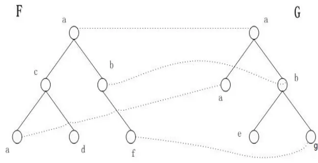
Figure 2.2: A forest edit mapping from F to G.

As shown in Figure 2.2, a mapping from F to G which consists of (1,1), (4,3), (5,4),

(6,5). If a pair of nodes is in the mapping, they are connected by a dot line. If a node

is not in the mapping(not touched by any line), it will be deleted or inserted. Later

in this thesis, if a pair of nodes is in the mapping, we say they are touched by a line.

Let I and J be the sets of nodes in F and G, respectively, not touched by any line in

M. Then the distance D of an edit mapping M is given by:

D(M)= P

(i,j)∈M

d(f[i],g[j]) + P i0_∈_I

d(f[i’],−)+ P j0_∈_J

d(−,g[j’]), where

I={i | there is no j that (i,j)∈ M }

J={ j | there is no i that (i,j)∈ M }

From all possible mappings, we define minimum cost mapping between F and G as

(20)

σ(F, G) = min { D(M) | M is a mapping between F and G }.

As mentioned above, we used a distance metric in the mapping. A similarity metric

also can be used in mapping. In this thesis, we use an edit similarity to replace the

edit distance and we use similarity scores instead of distance costs. The similarity

metric definition is described as: given a set A, a real-valued function s(a, b) on the

Cartesian product A × A is a similarity score if, for any a, b, c ∈ A, it satisfies the

following conditions:

(1) s(a, a) ≥ 0;

(2) s(a, b)= s(b, a);

(3) s(a, a) ≥ s(a, b);

(4) s(a, b)+ s(b, c) ≤s(b, b)+ s(a, c);

(5) s(a, a)= s(b, b)= s(a, b) if and only if a = b. [15]

Let the M to be a mapping from F to G. Let I and J be the sets of nodes in F and G,

respectively, not touched by any line in M. Then the similarity S of an edit mapping

M is given by:

S(M)= P

(i,j)∈M

s(f[i],g[j]) + P i0_∈_I

s(f[i’],−)+ P j0_∈_J

s(−,g[j’]), where

I={i | there is no j that (i,j)∈ M }

J={ j | there is no i that (i,j)∈ M }

The similarity metric can be extended to edit mapping from an alphabet. We use

φ(F, G) to represent the edit similarity between two forests throughout this thesis.

The definition of S making φ(F, G) a similarity metric between forests, is called a

forest edit similarity. To compute the forest edit similarity means to compute the

maximum score mapping which is denoted byφ(F, G).

(21)

Based on the five properties listed above, s(a, a)≥0 and φ(F, F)≥0. We usually set

s(-,-)=0 because there would be neither bonus nor penalty when mapping two nodes

with empty labels and setφ(∅, ∅)=0. So that s(a, -)≤0 and φ(F, ∅)≤0.[10]

2.4 Edit distance and edit similarity

The ordered edit distance metric was introduced by Tai [3]. Given two forestsF and

G, Tai presented an algorithm for the forest edit distance problem using O(|F| · |G| ·

DF2 ·DG2) time and O(|F| · |G|) space by using pre-order numbering. Zhang and

Shasha then presented a much simpler algorithm [7] which improved the running time

toO(|F| · |G| ·min{DF, LF} ·min{DG, LG}) by using post order numbering. In this

thesis, we use edit similarity with some modifications of edit distance.

Lemma 2.1 Let F, G be defined as above, l(i) is the leftmost descendent node of F(i)

(1) φ(∅,∅) = 0

(2) ∀i∈F,∀i0 ∈ {l(i), .., i},

φ(F[l(i)..i0],∅) = φ(F[l(i)..i0−1],∅) +s(f[i0],−).

(3) ∀j ∈G,∀j0 ∈ {l(j), .., j},

φ(∅, G[l(j)..j0]) = φ(∅, G[l(j)..j0−1]) +s(−, g[j0]).

Proof This is directly from Lemma 3 in [7].

We consider mapping from F[l(i)..i0] to G[l(j)..j0] and that mapping must respect

ancestor and sibling orders. If it includes a line fromf[i0] to g[j0] and (i0, j0) is in the

mapping, the mapping will consist of

(1) a mapping from the complete sub-tree F[i0] to the complete sub-tree G[j0].

(2) a mapping from the forest ofF with the complete sub-treeF[i0] removed to the

(22)

So we can have Lemma 2.2.

Lemma 2.2 [7] ∀(i, j)∈(F, G), ∀i0 ∈ {l(i), . . . , i} and ∀j0 ∈ {l(j), . . . , j},

φ(F[l(i)..i0], G[l(j)..j0]) = max

                    

φ(F[l(i)..i0−1], G[l(j)..j0]) +s(f[i0],−),

φ(F[l(i)..i0], G[l(j)..j0 −1]) +s(−, g[j0]),

φ(F[l(i)..l(i0)−1], G[l(j)..l(j0)−1])

+φ(F[l(i0)..i0−1], G[l(j0)..j0−1])

+s(f[i0], g[j0]).

Proof This is directly from Lemma 4 in [7].

To simplify the calculation ofφ(F[l(i)..i0], G[l(j)..j0]), consider two cases ofφ(F[l(i)..i0], G[l(j)..j0])

(1)F[l(i)..i0] and G[l(j)..j0] are both trees.

(2)F[l(i)..i0] or G[l(j)..j0] is a forest.

So that leti, j, F and G be defined as above,l(i)≤i0 ≤i and l(j)≤j0 ≤j

∀(i, j)∈(F, G),∀i0 ∈ {l(i), . . . , i} and ∀j0 ∈ {l(j), . . . , j}.

Ifl(i0) =l(i) and l(j0) = l(j),

φ(F[l(i)..i0], G[l(j)..j0]) = max

        

φ(F[l(i)..i0−1], G[l(j)..j0]) +s(f[i0],−),

φ(F[l(i)..i0], G[l(j)..j0−1]) +s(−, g[j0]),

φ(F[l(i)..i0−1], G[l(j)..j0 −1]) +s(f[i0], g[j0]).

Ifl(i0)6=l(i) and l(j0)6=l(j),

φ(F[l(i)..i0], G[l(j)..j0]) = max

        

φ(F[l(i)..i0−1], G[l(j)..j0]) +s(f[i0],−),

φ(F[l(i)..i0], G[l(j)..j0−1]) +s(−, g[j0]),

φ(F[l(i)..l(i0)−1], G[l(j)..l(j0)−1]) +φ(F[i0], G[j0]).

This is directly from Lemma 5 in [7].

Based on Lemma 2.1 and Lemma 2.2, we have Algorithm 1 and Algorithms 3 shown

(23)

Figure 2.3: Lemma 2.2[7]

Algorithm 1: T S(F, G) Input: Forest F and G.

Output: φ(F[i], G[j]), where 1≤i≤ |F| and 1≤j ≤ |G|.

1 for i:= 1 to |F| do

2 for j := 1 to |G| do

3 T reeSimilarity(i, j)

4 end

5 end

Zhang-Shasha’s algorithm also used the concept of key root [23]. Define k is a key

root node and the key root node set K of forest F as follows:

K(F) ={k|there exists no k0 > k such that l(k) =l(k0)}.

That is, if k is in K then either k is the root of F or k has a left sibling. Intuitively, this

set will be the roots of all the sub-trees of tree F that need separate computations. In

array K, the order of the elements is in increasing order. With the introduction of the

key roots [7] concept, we only need to compute T reeSimilarity(i, j) with i∈ K(F)

(24)

Algorithm 2: T reeSimilarity(i, j)

1 φ(∅,∅) = 0

2 for i0 :=l(i) to i do

3 φ(F[l(i)..i0],∅) =φ(F[l(i)..i0−1],∅) +s(f[i0],−)

4 end

5 for j0 :=l(j) to j do

6 φ(∅, G[l(j)..j0]) = φ(∅, G[l(j)..j0−1]) +s(−, g[j0])

7 end

8 for i0 :=l(i) to i do 9 for j0 :=l(j) to j do

10 if l(i0) =l(i) and l(j0) = l(j) then 11 φ(F[l(i)..i0], G[l(j)..j0]) =

max

 



φ(F[l(i)..i0−1], G[l(j)..j0]) +s(f[i0],−), φ(F[l(i)..i0], G[l(j)..j0−1]) +s(−, g[j0]), φ(F[l(i)..i0−1], G[l(j)..j0−1]) +s(f[i0], g[j0])

12 φ(F[i0], G[j0]) =φ(F[l(i)..i0], G[l(j)..j0])

13 else

14 φ(F[l(i)..i0], G[l(j)..j0]) =

max

 



φ(F[l(i)..i0−1], G[l(j)..j0]) +s(f[i0],−), φ(F[l(i)..i0], G[l(j)..j0−1]) +s(−, g[j0]),

φ(F[l(i)..l(i0)−1], G[l(j)..l(j0)−1]) +φ(F[i0], G[j0])

15 end

16 end

17 end

Algorithm 3: SZS(F, G) Input: Forest F and G.

Output: φ(F[i], G[j]), where 1≤i≤ |F| and 1≤j ≤ |G|.

1 compute K(F) andK(G) and sort them in increasing order into arraysK₁ and

K2, respectively

2 for i0 := 1 to |K₁| do 3 for j0 := 1 to |K₂| do

4 i:=K1[i0]

5 j :=K₂[j0]

6 T reeSimilarity(i, j)

7 end

(25)

Local Forest Similarity For

Sub-forests

Local forest similarity (LFS) aims at computing locally similar regions in two forests.

In this Chapter, we consider the LFS problem for forests which are sequences of

sub-trees. The roots of the sub-trees are nodes of the forests. Given two ordered labelled

forestsF andG, the local forest similarity problem is to determine sub-forestsF0 and

G0 of F and G respectively such that they are the most similar over the all possible

F0 and G0.

The algorithm of LFS is to compute the maximum score of the following formula,

LF S(F, G)=max

F0_,G0φ(F

0_{, G}0₎

F0 ∈subf(F)

G0 ∈subf(G).

3.1 The algorithm for local sequence similarity and

longest common sub-sequence

Sequences are a special case of trees/forests. A sequence can be considered as a linear

tree or a forest so that all the trees in it have only one node. For sequence, the LFS

problem becomes a local sequence similarity problem when we consider it as a linear

(26)

Chapter 3. Local Forest Similarity For Sub-forests 17

tree and weighted longest common sub-sequence problem when we consider it as a

forest of singleton trees.

Local sequence similarity (LSS) problem [2] is to determine two sub-sequences from

two given sequences such that they are most similar. Figure 3.1 shows the local

sequence alignment.

The problem is defined below.

Figure 3.1: Local sequence similarity alignment.

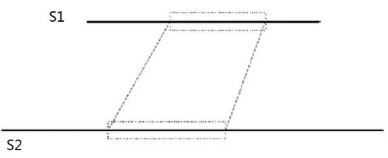
Given two sequencesS1[1..m],S2[1..n], SMS computes the maximum score using the

following the formula

SM S(S1, S2)=max{φ(S1[i..j], S2[k..l])|1≤i≤j ≤m,1≤k ≤l≤n}

Dynamic programming was used to solve this problem by Smith and Waterman [2].

They also give another interpretation of the LSS problem. The SM S(i, j) is the

maximum similarity score of two segments ending at S1[i], S2[j]

SM S(i, j)=max

i0_,j0 {0;φ(S1[i

0_..i_]_{, S}

2[j0..j])|1≤i0 ≤i,1≤j0 ≤j}

The SM S(S1, S2) is defined as follow:

SM S(S1, S2)=max

(27)

Algorithm 4: Local sequence similarity

Input: S1,S2, All the s(i,−) ,s(−, j),s(i, j) where i, j ≥0

Output: maxφ(S1[i0..i], S2[l0..l]), where 1≤i0 ≤i≤ |S1|,1≤j0 ≤j ≤ |S2|.

1 for i= 0 to |S₁| do 2 φ[i,0] = 0

3 end

4 for j = 0 to |S₂| do 5 φ[0, j] = 0

6 end

7 for i= 1 to |S₁| do

8 for j = 1 to |S₂| do

9 φ(i, j) = max

       0,

φ(i−1, j−1) +s(i, j), φ(i−1, j) +s(i,−), φ(i, j−1) +s(−, j).

10 end

11 end

As Algorithm 4 shows, consider the optimal solution, there are two segments ending

at (i, j). In the dynamic program matrix, initial deletions ofS2 are set at φ[0, j] = 0.

Initial insertions ofS1 are set atφ[i,0] = 0. Think of the all possible segments ending

at(i, j), if φ(i−1, j−1) +s(i, j), φ(i−1, j) +s(i,−), φ(i, j−1) +s(−, j) ends with

all negative values, then there is no positive scoring segment ending at (i, j) and the

value is 0 since the optimal solution is two empty segments. If there is one or more

positive scoring segments ending at (i, j), (i, j) is in the alignment. We pick the

largest positive score as an optimal path.

The longest common subsequence (LCS) problem is to compute the longest

sub-sequence common between two sub-sequences. Figure 3.2 shows the longest common

sub-sequence. Given two sequencesS1[1..m] and S2[1..n], Algorithm 5 computes the

maximum length of the LCS by using dynamic programming. From Algorithm 5,

to compute the longest common sub-sequences toC[i, j], compare the elements S1[i]

and S2[j]. If they are equal, then the sequence C[i−1, j −1] is extended by that

element. If they are not equal, then the longer of the two sequences, C[i−1, j] and

(28)

Figure 3.2: Longest common sub-sequence

Algorithm 5: Longest common sub-sequence Input: S1,S2, C[|S1|][|S2|] = 0

Output: LCS

1 for i= 0 to |S1| do

2 C[i,∅] = 0

3 end

4 for j = 0 to |S2| do

5 C[∅, j] = 0

6 end

7 for i= 1 to |S1| do

8 for j = 1 to |S₂| do

9 if S₁[i]=S₂[j], then

10 C[i, j] =C[i−1, j−1] + 1

11 end

12 if S₁[i]6=S₂[j], then 13 C[i, j] = max

C[i−1, j]

C[i, j−1]

14 end

15 end

16 end

3.2 Forest removing similarity for sub-forests

From the definition, we want to compute sub-forests F0 and G0. An ordered labelled

forest is a sequence of ordered labelled trees. The unit of the sequence is a sub-tree.

In the computation, we actually need to determine a sequence of nodes, i1, i2, ...im

(29)

Lemma 3.1 Given the forests F and G, let i1, i2, ...im be sequence of nodes of F. let j1, j2, ...jm be a sequence of nodes of G, then

LF S(F, G)= max

i1,...im,j1...jm,m

m P

k=1 max

f,g φ(F[ik]\f, G[jk]\g) f ∈subcf(F[ik], ik), g ∈subcf(G[jk], jk)

1 ≤ m ≤min(|F|,|G|)

1 ≤ik≤ |F|, 1 ≤jk ≤ |G|

Proof SupposeF0 andG0are the optimal solution such that they can make maximum

LF S(F, G).

LF S(F, G)=max

F0_,G0φ(F

0_{, G}0₎

F0 ∈subf(F)

G0 ∈subf(G)

Both sub-forests F0 and G0 are sequence of sub-trees. Each sub-tree has a root.

φ(F0, G0) is a mapping from F0 to G0. Assume all the roots are in the mapping and

roots ofF0 map with roots ofG0. If not, there is one or more roots not in the mapping,

then they could be deleted. Situations like this will cost score penalty which is

non-positive. So removing of these nodes will not make the score worse. F0 and G0 are

ordered labelled forests. The root of the first sub-tree in F0 must map with the root

of the first sub-tree in G0, and the rest of the roots map with each other according

to the order. Consider all roots are in the mapping and map according to the order,

the number of sub-trees ofF0 should be equal with the number of sub-trees ofG0.

Consider a pair nodesik and jk fromφ(F0, G0) mapping with each other, the score is

φ(F[ik]\f, G[jk]\g). φ(F0, G0) should be the sum of each pair of sub-tree’s maximum

edit similarity score. Normally, maxφ(F0, G0) will be larger than 0. If not, the best

mapping is empty tree.

Suppose there are m sub-trees in F0 and G0 respectively.

φ(F0, G0)=

m P

n=1 max

(30)

LF S(F, G)= max

i1,...im,j1...jm,m

m P

k=1 max

1 ≤ m≤min(|F|,|G|)

1≤ik ≤ |F|, 1≤jk ≤ |G|

From Lemma 3.1, in order to compute LF S(F, G), two steps are necessary. First

step, compute all the φ(F[ik]\f, G[jk]\g). Second step, select several(m) φ(F[ik]\

f, G[jk]\g) such that the sum of the scores are optimal. For the first step, to calculate

φ(F[ik]\f, G[jk]\g), we extend Smith and Waterman’s LSS algorithm from sequences

to trees. In their LSS algorithm, they removed prefix of the sub-sequence. In our

algorithm, complete sub-trees can be removed without penalty. In this section, we

propose forest removing similarity(FRS) for sub-forests algorithm to calculate the

maximum similarity scores of allF[i] andG[j] when some sub-forests can be removed

from both of F[i] and G[j].

The problem is defined as follows:

Given two forests F and G, FRS for sub-forests

Φrr(F[i], G[j]) = max

f,g φ(F[i]\f, G[j]\g) f ∈subcf(F[i], i)

g ∈subcf(G[j], j)

The subscript “rr” represents that sub-forests or children nodes of both F and G can

be removed.

We use the formula from [7]

For Φrr(F[l(i)..i0], G[l(j)..j0]), where l(i)≤i0 ≤i and l(j)≤j0 ≤j.

(a) Φrr(∅,∅) = 0.

(b) Φrr(F[l(i)..i0],∅) = 0.

(31)

(d) Φrr(F[l(i)..i0], G[l(j)..j0]) = max                           

Φrr(F[l(i)..l(i0)−1], G[l(j)..j0]),

Φrr(F[l(i)..i0], G[l(j)..l(j0)−1]),

Φrr(F[l(i)..i0−1], G[l(j)..j0]) +s(f[i0],−),

Φrr(F[l(i)..i0], G[l(j)..j0−1]) +s(−, g[j0]),

Φrr(F[l(i)..l(i0)−1], G[l(j)..l(j0)−1])

+ Φrr(F[l(i0), i0−1], G[l(j0), j0−1]) +s(f[i0], g[j0]).

For case(a), edit operation is not required. For case(b), F[l(i)..i0] can be removed

so that no edit operation required. For case(c),G[l(j)..j0] can be removed so that no

edit operation required .

For case(d), five cases should be considered

For the Φrr(F[l(i)..i0], G[l(j)..j0]), five cases should be considered

Case 1: whether or not the sub-tree F[l(i0)..i0] is removed.

Case 2: whether or not the sub-tree G[l(j0)..j0] is removed.

If it is not one of the cases above, consider the optimal mapping M betweenF[l(i)..i0]and

G[l(j)..j0] after we perform an optimal removal of sub-trees ofF[l(i)..i0] andG[l(j)..j0].

The mapping can be extended tof[i0], and g[j0] in three ways

Case 3: f[i0] is not touched by a line in M, then (i0,−)∈M.

Case 4: g[j0] is not touched by a line in M, then (−, j0)∈M.

Case 5: f[i0] and g[j0] are both touched by lines in M, then (i0, j0)∈M.

This is directly from[7].

To simplify the calculation ofφ(F[l(i)..i0], G[l(j)..j0]), consider two cases ofφ(F[l(i)..i0], G[l(j)..j0])

(1) F[l(i)..i0] and G[l(j)..j0] are both trees.

(2) F[l(i)..i0] or G[l(j)..j0] is a forest.

Leti, j, F and Gbe defined as above, l(i)≤i0 ≤i and l(j)≤j0 ≤j

(32)

Φrr(F[l(i)..i0], G[l(j)..j0]) = max                0

Φrr(F[l(i)..i0−1], G[l(j)..j0]) +s(f[i0],−),

Φrr(F[l(i)..i0], G[l(j)..j0 −1]) +s(−, g[j0]),

Φrr(F[l(i)..i0−1], G[l(j)..j0−1]) +s(f[i0], g[j0]).

Φrr(F[l(i)..i0], G[l(j)..j0]) = max                     

Φrr(F[l(i)..l(i0)−1], G[l(j)..j0]),

Φrr(F[l(i)..i0], G[l(j)..l(j0)−1]),

Φrr(F[l(i)..i0−1], G[l(j)..j0]) +s(f[i0],−),

Φrr(F[l(i)..i0], G[l(j)..j0 −1]) +s(−, g[j0]),

Φrr(F[l(i)..l(i0)−1], G[l(j)..l(j0)−1]) + Φrr(F[i0], G[j0]).

This algorithm can be implemented to run inO(|F|·|G|·min{DF, LF}·min{DG, LG})

time and O(|F| · |G|) space by using the Zhang-Shasha algorithm.

Zhang-Shasha-RemovingSimilarity is an efficient method to solve tree removing

simi-larity problem. Φrr(F[i0], G[j0]) is the key data of LFS problem and is needed in next

section.

Algorithm 6: RemovingSimilarity(F, G) Input: Forest F and G.

Output: Φrr(F[i], G[j]), where 1≤i≤ |F| and 1≤j ≤ |G|.

1 compute K(F) andK(G) and sort them in increasing order into arraysK₁ and

K2 respectively.

2 for i0 := 1 to |K1| do

3 for j0 := 1 to |K₂| do

4 i:=K₁[i0]

5 j :=K₂[j0]

6 T reeRemovingSimi(i, j)

7 end

(33)

Algorithm 7: T reeRemovingSimi(i, j)

1 Φrr(∅,∅) = 0

2 for i0 :=l(i) to i do 3 Φ_rr(F[l(i)..i0],∅) = 0

4 end

5 for j0 :=l(j) to j do 6 Φ_rr(∅, G[l(j)..j0]) = 0

7 end

10 if l(i0) =l(i) and l(j0) = l(j) then 11 Φ_rr(F[l(i)..i0], G[l(j)..j0]) =

max        0,

Φrr(F[l(i)..i0−1], G[l(j)..j0]) +s(f[i0],−),

Φrr(F[l(i)..i0], G[l(j)..j0−1]) +s(−, g[j0]),

Φrr(F[l(i)..i0−1], G[l(j)..j0−1]) +s(f[i0], g[j0])

12 Φrr(F[i0], G[j0]) = Φrr(F[l(i)..i0], G[l(j)..j0])

13 else

14 Φrr(F[l(i)..i0], G[l(j)..j0]) =

max               

Φrr(F[l(i)..l(i0)−1], G[l(j)..j0]),

Φrr(F[l(i)..i0], G[l(j)..l(j0)−1]),

Φrr(F[l(i)..i0−1], G[l(j)..j0]) +s(f[i0],−),

Φrr(F[l(i)..i0], G[l(j)..j0−1]) +s(−, g[j0]),

Φrr(F[l(i)..l(i0)−1], G[l(j)..l(j0)−1])

+ Φrr(F[i0], G[j0])

15 end

16 end

(34)

3.3 Our algorithms for local forest similarity

In this section, we modify the weighted longest common sub-sequence algorithm and

use it on trees to calculate LF S(F, G), the second step mentioned in Lemma 3.1. A

matrix DP[|F|][|G|] is designed to calculate LF S(F, G) by using dynamic

program-ming.

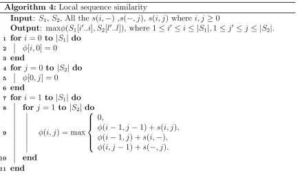
Lemma 3.2 Define i is ith node in F, j is jth node in G,

DP(i, j) = LF S(F[1...i], G[1...j]), DP[i,∅] = 0, DP[∅, j] = 0 then

DP(i, j) = max

        

DP(i−1, j)

DP(i, j−1)

DP(l(i)−1, l(j)−1) + Φrr(F[i], G[j])

Proof Consider the optimal solution mapping of F[1...i] and G[1...j], supposei1, ...im, j1...jmare the optimal sub-tree’s roots of optimal solution mapping. ComputeDP(i, j),

to determine whether or not node i is im and whether or not node j is jm. Case 1,

nodei is not im. The maximum similarity score is from F[1...i−1], G[1...j]. Case 2,

node j is not jm. The maximum similarity score is from F[1...i], G[1...j −1]. Case

3, node i is im and node j is jm. Both f[i] and g[j] are in the mapping so that they

are the last pair till (i,j). From definitions above, F[i] and G[j] should be mapping

with each other. The optimal edit similarity mapping score is Φrr(F[i], G[j]) so that

DP(i, j) = DP(l(i)−1, l(j)−1) + Φrr(F[i], G[j]).

Figure 3.3 shows three cases of computation for local forest similarity ofF[1...i], G[1...j].

(35)

Figure 3.3: Local forest similarity operations

Algorithm 8: Local forest similarity for sub-forest

Input: forest F and GΦrr(F[i], G[j]) where 1≤i≤ |F| and 1≤j ≤ |G|

Output: DP[|F|][|G|]

1 for i= 0 to |F| do 2 DP[i,∅] = 0

3 end

4 for j = 0 to |G| do 5 DP[∅, j] = 0

6 end

7 for i= 1 to |F| do

8 for j = 1 to |G| do

9 DP(i, j) = max

 



DP(i−1, j)

DP(i, j−1)

DP(l(i)−1, l(j)−1) + Φrr(F[i], G[j])

10 end

11 end

The local forest similarity for sub-forest algorithm shows how similar F and G are.

(36)

is needed and the mapping can be calculated by Algorithm 9.

T RStraceback is a procedure used in Algorithm 9. The main idea of T RStraceback

algorithm is to calculate Φrr(F[i], G[j]) by usingT reeRemovingSimilarityalgorithm

and using a matrix which is large enough (|F| ∗ |G|) for storing intermediate results.

Then, use the matrix to determine the optimal result. When tracebacked to i and

j, the algorithm determines whether or not they are involved. If so , T RStraceback

algorithm calculates how F[i] and G[j] are mapped with each other by calculating

the sequence of mapping operations (insertion\deletion\mapping) so that the optimal

solution can be achieved.

Algorithm 9: Traceback Input: Matrix DP[|F|][|G|] Output: maxφ(F \f, G\g)

1 i=|F| 2 j=|G|

3 while i 6= 0 and j 6=0 do

4 if DP[i][j] ==DP[i][j−1]then

5 j− −;

6 Continue;

7 end

8 if DP[i][j] ==DP[i−1][j]then

9 i− −;

10 Continue;

11 end

12 if DP[i][j] ==DP[l[i]−1][l[j]−1] + Φ_rr(F[i], G[j]) then 13 if Φ_rr(F[i], G[j])>0 then

14 T RStraceback(i, j);

15 end

16 i=l[i]−1;

17 j =l[j]−1;

18 Continue;

19 end

20 end

In this Chapter, we have introduced our algorithm for forest removing similarity

(37)

Forest Pattern Matching For

Sub-forests

Forest pattern matching (FPM) aims at computing regions of forestF which are most

similar to another forest G. Generally, F is much larger than G. In this chapter, we

consider the FPM problem. Given two ordered labelled forests F and G, the forest

pattern matching for sub-forest problem is to determine sub-forestF0 of F such that

it is the most similar toG over all the possible F0 .

The goal of FPM for sub-forests is to compute the maximum score of the following

formula,

F P M(F, G)=max

F0 φ(F

0_{, G}₎

F0 ∈subf(F)

4.1 The algorithm for sequence pattern matching

It is known from section 3.1 that a sequence is a special case of a tree/forest. In this

section, we introduce the pattern matching problem on sequences.

Sequence pattern matching (SPM) is to compute the best fit of a “short” sequence

into a “longer” sequence. The SPM algorithm computes where the short pattern

ap-proximately appears in the longer sequence. Consider the problem of fitting sequence

(38)

Chapter 4. Forest Pattern Matching For Sub-forests 29

A = a1...an into B = b1...bm where n is much smaller than m. The problem is to

compute

SP M(A, B)= max{φ(A, bkbk+1...bl−1bl) : 1 ≤k≤l ≤m}

Figure 4.1: Sequence pattern matching

From Figure 4.1, we take another approach. Note that deletions of the beginning and

the end of B are without penalty. Define

SP M(i, j) = max

k,j {φ(a1a2...ai−1ai, bkbk+1...bj−1bj) : 1 ≤k≤j ≤m, i =n}

Deletions of the beginning of B without penalty can be encoded when a dynamic

programming matrix is set up. The score of the initial deletion of B ,b1b2...bj, is set

at φ[0, j] = 0. Each letter of A must be accounted for so that φ[i,0]=−i∗s(i,−).

After initial matching, deletion at the end of B as well as A must be accounted for.

Choose the best score ofSP M(i, j) from φ(i−1, j−1) +s(i, j), φ(i−1, j) +s(i,−)

and φ(i, j−1) +s(−, j) [11].

Two sequences are given as examples, and set s(a, a) = 1, s(a, b) = −1, s(a,−) =

s(−, a) =−2. Figure 4.2 shows the result of sequence pattern matching compued by

Algorithm 10.

A=TATAAT

(39)

Algorithm 10: Sequence Pattern Matching

Input: sequenceA and B, All the s(i,−) ,s(−, j), s(i, j) wherei, j ≥0 Output: max{φ(a1a2...ai−1ai, bkbk+1...bl−1bl)}

1 φ[∅,∅] = 0

2 for i= 1 to |A| do

3 φ[i,∅] =φ[i−1,∅] +s(i,−)

4 end

5 for j = 1 to |B| do 6 φ[∅, j] = 0

7 end

8 for i= 1 to |S₁| do

9 for j = 1 to |S2| do

10 φ(i, j) = max

 



φ(i−1, j−1) +s(i, j), φ(i−1, j) +s(i,−), φ(i, j−1) +s(−, j).

11 end

12 end

(40)

4.2 Forest pattern matching for sub-forests

Given two forests F and G where F is larger than G, we use two steps to compute

FPM. Step 1, we compute the the forest pattern matching for each pair of sub-trees

between F and G. Step 2, we extend sequence pattern matching algorithm from

sequences to forests.

In sequence pattern matching, the deletion of the short sequence will cost a penalty.

In forest pattern matching, given two forestsF and G whereF is larger than G, the

deletion of any node in G will cost a penalty. The prefix of the larger sequence’s

sub-sequence can be removed in SPM. In our algorithm, complete sub-trees can be

removed from F without penalty. Define FPMSS as follows

F P M SS(F[ik], G[jk])=max

f φ(F[ik]\f, G[jk]) f ∈subcf(F[ik]).

In this section, we propose the forest pattern matching (FPM) for sub-forests

algo-rithm to calculateF P M SS(F[i], G[j]) of allF[i] andG[j] when some sub-forests can

be removed from F[i].

The problem is defined as follows:

Given two forests F and G,F is larger thanG, FPM for sub-forests

ΦR(F[i], G[j]) = max

f φ(F[i]\f, G[j]) f ∈subcf(F[i])

The subscript “R” represents that only sub-forests or child nodes ofF can be removed.

To simplify the calculation of ΦR(F[i], G[j]), consider two cases ofφ(F[l(i)..i0], G[l(j)..j0])

(1) F[l(i)..i0] and G[l(j)..j0] are both trees.

(2) F[l(i)..i0] or G[l(j)..j0] is a forest.

Leti,j F and G be defined as above,l(i)≤i0 ≤i and l(j)≤j0 ≤j

(41)

ΦR(F[l(i)..i0], G[l(j)..j0]) = max         

ΦR(F[l(i)..i0−1], G[l(j)..j0]) +s(f[i0],−),

ΦR(F[l(i)..i0], G[l(j)..j0 −1]) +s(−, g[j0]),

ΦR(F[l(i)..i0−1], G[l(j)..j0−1]) +s(f[i0], g[j0]).

ΦR(F[l(i)..i0], G[l(j)..j0]) = max               

ΦR(F[l(i)..l(i0)−1], G[l(j)..j0])

ΦR(F[l(i)..i0−1], G[l(j)..j0]) +s(f[i0],−),

ΦR(F[l(i)..i0], G[l(j)..j0 −1]) +s(−, g[j0]),

ΦR(F[l(i)..l(i0)−1], G[l(j)..l(j0)−1]) + ΦRr(F[i0], G[j0]).

In the local similarity calculations, prefix of the sub-sequence can be deleted without

penalty. If the two sub-forests or sub-sequences are not quite similar (negative), their

scores are set to 0. But in pattern matching, it can be negative because the deletion

of the smaller forest costs penalty.

This algorithm can be implemented to run inO(|F|·|G|·min{DF, LF}·min{DG, LG})

time and O(|F| · |G|) space by using Zhang-Shasha algorithm.

Algorithm 11: F P M SS(F, G) Input: Forest F and G.

Output: ΦR(F[i], G[j]), where 1≤i≤ |F| and 1≤j ≤ |G|.

1 compute K(F) andK(G) and sort them in increasing order into arraysK1 and

K2 respectively.

2 for i0 := 1 to |K₁| do 3 for j0 := 1 to |K2| do

4 i:=K₁[i0]

5 j :=K₂[j0]

6 F P M SSP rocedue(i, j)

7 end

(42)

Algorithm 12: F P M SSP rocedue(i, j)

1 Φ_R(∅,∅) = 0

2 for i0 :=l(i) to i do 3 ΦR(F[l(i)..i0],∅) = 0

4 end

5 for j0 :=l(j) to j do

6 ΦR(∅, G[l(j)..j0]) =G[l(j)..j0−1]) +s(−, g[j0])

7 end

10 if l(i0) =l(i) and l(j0) = l(j) then 11 Φ_R(F[l(i)..i0], G[l(j)..j0]) =

max

 



ΦR(F[l(i)..i0 −1], G[l(j)..j0]) +s(f[i0],−),

ΦR(F[l(i)..i0], G[l(j)..j0−1]) +s(−, g[j0]),

ΦR(F[l(i)..i0 −1], G[l(j)..j0 −1]) +s(f[i0], g[j0])

12 ΦR(F[i0], G[j0]) = ΦR(F[l(i)..i0], G[l(j)..j0])

13 else

14 ΦR(F[l(i)..i0], G[l(j)..j0]) =

max           

ΦR(F[l(i)..l(i0)−1], G[l(j)..j0]),

ΦR(F[l(i)..i0 −1], G[l(j)..j0]) +s(f[i0],−),

ΦR(F[l(i)..i0], G[l(j)..j0−1]) +s(−, g[j0]),

ΦR(F[l(i)..l(i0)−1], G[l(j)..l(j0)−1])

+ ΦR(F[i0], G[j0])

15 end

16 end

(43)

4.3 Our algorithms for forest pattern matching

In this section, we design an algorithm to compute theF P M. A matrix DP[|F|][|G|]

is used to calculateF P M(F, G) by using dynamic programming.

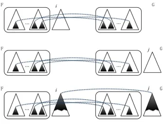
Lemma 4.1 Define i is ith node in F, j is jth node in G,

DP(i, j) = F P M(F[1...i], G[1...j]), DP[i,∅] = 0, DP[∅, j] =DP[∅, j−1])+s(−, g[j]),

then

DP(i, j) = max

    

   

DP(i−1, j)

DP(i, j−1) +s(−, g[j])

DP(l(i)−1, l(j)−1) + ΦR(F[i], G[j])

Proof Consider the optimal solution mapping of F[1...i] and G[1...j], supposej1...jm

are optimal solutions mapping sub-tree’s roots inGand they have no parent node in

the mapping. i1, ...im are corresponding nodes in F. ComputeDP(i, j), to determine

whether or not nodeiisim and whether or not nodej isjm. Case 1, nodeiis not im.

The maximum pattern matching score is fromF[1...i−1], G[1...j]. Case 2, node j is

not jm. The maximum pattern matching score is from F[1...i], G[1...j −1] plus the

penalty of deleting j. Case 3, node i is im and node j is jm. Both f[i] and g[j] are

in the mapping so that they are the last pair till (i,j). From definitions above, F[i]

and G[j] should be mapped with each other. The optimal pattern matching score is

ΦR(F[i], G[j]) so that DP(i, j) =DP(l(i)−1, l(j)−1) + ΦR(F[i], G[j])

Figure 4.3 shows three cases of computation for forest pattern matching ofF[1...i], G[1...j].

(44)

Figure 4.3: Forest pattern matching operations

The traceback method is the same as for LFS problem. In this Chapter, we

intro-duce our algorithm for forest pattern matching problem. The implementation and

experimental results are in Chapter 5.

Algorithm 13: Forest pattern matching

Input: forest F and GΦRr(F[i], G[j]) where 1≤i≤ |F|and 1≤j ≤ |G|

Output: DP[|F|][|G|]

1 for i= 0 to |F| do 2 DP[i,∅] = 0

3 end

5 DP[∅, j] =DP[∅, j−1]) +s(−, g[j])

6 end

7 for i= 1 to |F| do

9 DP(i, j) = max

 



DP(i−1, j)

DP(i, j−1) +s(−, g[j0])

DP(l(i)−1, l(j)−1) + ΦRr(F[i], G[j])

10 end

(45)

Implementation and Experimental

Results

In this Chapter, we present the implementation of the algorithms of LFS and FPM

for sub-forests and experimental results.

5.1 Implementation

A C++ program is written for the algorithms. First, user needs to choose either LFS

or FPM for the calculation. Second, user has to type in the names of score matrix

file and forest data file. The program will begin the calculation automatically if the

two files can be found successfully. At last, user has to type in a file name. All the

results will be written in the file. Figure 5.1 shows the flowchart of the program.

(46)

Chapter 5. Implementation and Experimental Results 37

(47)

5.2 Experimental results and discussion

Five experiments are designed to test the algorithm. Experiment 1, 2 and 5 are for

LFS and experiment 3 and 4 are for FPM.

Pseudoknot-free RNA can be represented as forests. Our forest data are taken from

RNA cupriavidus metallidurans and streptomyces bikiniensis. Cupriavidus

metal-lidurans and streptomyces bikiniensis, the RNase P RNA structures of bacteria, are

pseudoknot-free. Cupriavidus metallidurans are renamed from ralstonia

metallidu-rans and previously known as ralstonia eutropha and alcaligenes eutrophus. The

images are taken from the website http://www.mbio.ncsu.edu/RNaseP/.

A forest data file has two sections. The first section represents the forest which is

also the primary structure of forest. The second section contains all the information

of forest’s secondary structure such as the start bases, end bases, stem size etc.. A

‘<’ sign alone on a line separates the two sections.

The score matrix file is significant such that results can be different by using different

score matrix for the same forests. In our experiments, we use the same score matrix

to test our algorithm. As shown in figure 5.2, the scores are set that match is 2,

mismatch is -1, insertion and deletion is -2 for each single base. For a base pair,

match is 4, mismatch is -2, insertion and deletion is -4. The penalty of matching

a single base to a base pair is -9 since it is not reasonable. A high penalty score

setting up can avoid this situation during the computation. Note that the scores are

3 when AU matches UA, CG matches GC and GU matches UG since these kinds of

matches are treated as the good cases in RNA computing although the base pairs

are not exactly the same. When the other reasonable base pairs match with each

other, we set the score to 1 because they are common situations in regard of RNA

secondary structures. ‘ - ’ represents insertion and deletion and ‘ ’ represents the

base is removed.

(48)

(49)

Experiment 1 Forest file:

Figure 5.3: forest file for experiment 1.

Result file:

(50)

Figure 5.5: Result of experiment 1.

In experiment 1, we use two small trees to test the program. Figure 5.5 shows the

result. The program determines one sub-forest from each tree and the maximum

similarity score is 70. 5 sub-trees with one single base are removed from Tree 1 and

6 from Tree 2. One base pair of Tree 1 maps to insertion/deletion. One complete

sub-tree of Tree 2 is totally removed. As the graph shows, the program determines

(51)

(52)

Result file:

(53)

(54)

In experiment 2, we input two whole large RNAs, cupriavidus metallidurans and

streptomyces bikiniensis.

The result is shown in Figure 5.8. Three sub-trees are determined from each RNA.

Two of them are sub-trees which have only one single base. The other ones are large

trees with some of its sub-trees removed.

From the detail, we can see there are other solutions, especially at loop structure

(multiple loop, hairpin loop etc.). In fact, for all kinds of similarity calculation, the

optimal solution may not be unique. To LSS, the maximum score may appear more

than once in the matrix. In LFS, for each point in the matrix, operations may get the

same score. But all these solutions are correct at the algorithm level. Our algorithm

(55)

(56)

Result file:

(57)

In experiment 3, we pick up two complete sub-forests and combine them to a forest.

Then fit it to alcaligenes eutrophus. Figure 5.11 shows the result of experiment 3.

Two parts of the structure are determined. One single base from the first part is

(58)

(59)

Result file:

(60)

In experiment 4, we fit a closed sub-forest from streptomyces bikiniensis to alcaligenes

eutrophus. Figure 5.14 shows the result of experiment 4. 9 sub-trees are determined.

Two single bases from the sub-trees are removed. Two single bases from the pattern

(61)

Figure 5.15: forest file for experiment 5.

Result file:

(62)

Experiment 5 is for LFS problem. We pick a small sub-forest from Alcaligenes

eu-trophus and Streptomyces bikiniensis respectively. 19 sub-trees are found out of each

sub-forest.

As Figure 5.17 shows, the 1st to 10th sub-trees are siblings in the first sub-forest. But

the 1st to 10th sub-trees are not siblings in the second sub-forest. The mapping of

the 4th to 8th sub-trees may not make sense in RNA structure. And also, the similar

situation also appears in Experiment 4 that the first ‘G’ is located far away from

oth-ers. All these solutions are correct at the algorithm level. The result of Experiment

5 is a typical solution that is correct in algorithm but may not be reasonable in RNA

(63)

Conclusion

In this thesis, we studied local forest similarity and forest pattern matching problems.

We developed efficient algorithms for general cases of these two problems.

For the local forest similarity problem, based on the well known Smith-Waterman

method for local sequence similarity and longest common sub-sequence algorithm, we

designed new algorithms to extend them from sequence to forest. Many algorithm

techniques can be used for the tree removing similarity algorithm and we chose the

Zhang-Shasha method in our algorithms. Our algorithm can identify locally similar

regions in two forests.

For the forest pattern matching, based on sequence pattern matching we designed

new algorithms to extend it from sequence to forest. Our algorithm can identify

regions from one large forest which are most similar to another small forest.

Both the local forest similarity algorithm and the forest pattern matching algorithm

can be applied to RNA structure comparison since pseudoknot-free RNA can be

represented as forests.

Our algorithm can determine the general case of local forest similarity and forest

pattern matching problems. In some cases, as the experiments showed, sub-forest

determination is split over the forest. But a compact result may be more reasonable

in RNA structure comparison. A possible way is to add the gap penalty during the

computation. We will continue to improve our algorithm in the future research.

(64)

Bibliography

[1] B. A. Shapiro and K. Zhang. Comparing multiple RNA secondary structures

using tree comparisons. Computer Applications in the Biosciences, 6(4):309–

318, 1990.

[2] T. F. Smith and M. S. Waterman. Identification of common molecular

subse-quences. Journal of Molecular Biology, 147(1):195–197, 1981.

[3] K.-C. Tai. The tree-to-tree correction problem. Journal of the Association for

Computing Machinery(JACM), 26(3):422–433, 1979.

[4] R. A. Wagner and M. J. Fischer. The string–to–string correction problem.

Jour-nal of the Association for Computing Machinery (JACM), 21(1):168–173, 1974.

[5] J. Wang, B. A. Shapiro, D. Shasha, K. Zhang, and K. M. Currey. An algorithm

for finding the largest approximately common substructures of two trees. IEEE

Trans. Pattern Anal. Mach. Intell., 20(8):889–895, 1998.

[6] K. Zhang. Computing similarity between RNA secondary structures. In

Proceedings of IEEE International Joint Symposia on Intelligence and

Sys-tems,Rockville, Maryland, May 1998, pages 126–132.

[7] K. Zhang and D. Shasha. Simple fast algorithms for the editing distance between

trees and related problems.SIAM Journal on Computing, 18(6):1245–1262, 1989.

[8] K. Zhang and Y. Zhu. Algorithms for Forest Pattern Matching. In Proceedings

of the 21th Symposium on Combinatorial Pattern Matching(CPM 2010), pages

1–12, 2010.

(65)

[9] Y. Zhu. Algorithms for Forest Pattern Matching and Local Forest Similarity.

Thesis(M.Sc), School of Graduate and Postdoctoral Studies, University of

West-ern Ontario, London, Ontario, Canada, 2010.

[10] Liang, Z Efficient algorithms for local forest similarity Thesis (M. Sc), School

of Graduate and Postdoctoral Studies, University of Western Ontario, London,

Ontario, Canada 2011.

[11] Waterman, Michael S Introduction to computational biology: maps, sequences

and genomes Book, CRC Press, 1995.

[12] J. W. Brown. The Ribonuclease P Database. Nucleic Acids Research, 27(1):314,

1999.

[13] R. Backofen and S. Will. Local Sequence-structure Motifs in RNA. Journal of

Bioinformatics and Computational Biology, 2(4):681–698, 2004.

[14] T. Bray, J. Paoli, C.M. Sperberg-McQueen, E. Maler, and F. Yergeau, Extensible

markup language (XML) 1.0. W3C recommendation, 6, 2000.

[15] S. Chen. Topics in Computing Similarity and Distance. Thesis(Ph.D), School

of Graduate and Postdoctoral Studies, University of Western Ontario, London,

Ontario, Canada, 2008.

[16] S. Chen, B. Ma, and K. Zhang On the similarity metric and the distance metric.

Theor. Comput. Sci. 410(24-25):2365–2376, 2009.

[17] E. D. Demaine, S. Mozes, B. Rossman, and O. Weimann. An optimal

decompo-sition algorithm for tree edit distance. In Proceedings of the 34th International

Colloquium on Automata, Languages and Programming(ICALP), pages 146–157,

2007.

[18] M. H¨ochsmann, T. T¨oller, R. Giegerich, and S. Kurtz. Local similarity in RNA

secondary structures. InProceedings of the IEEE Computational Systems

(66)

BIBLIOGRAPHY 57

[19] J. Jansson, N. T. Hieu, and W.K. Sung. Local Gapped Subforest Alignment and

Its Application in Finding RNA Structural Motifs. Journal of Computational

Biology, 13(3): 702–718, 2006.

[20] J. Jansson and Z. Peng. Algorithms for Finding a Most Similar Subforest. In

Proceedings of the 17th Symposium on Combinatorial Pattern Matching, pages

377–388, 2006.

[21] T. Jiang, L. Wang, and K. Zhang. Alignment of trees - an alternative to tree

edit. Theoretical Computer Science, 143:137–148, 1995.

[22] P. N. Klein. Computing the edit-distance between unrooted ordered trees. In

Proceedings of the 6th European Symposium on Algorithms (ESA 1998), pages

91–102, 1998.

[23] Motifs database. http://subviral.med.uottawa.ca/cgi-bin/motifs.cgi.

[24] Z. Peng. Algorithms for Local Forest Similarity. In Proceedings of the 16th

International Symposium on Algorithms and Computation(ISAAC 2005), pages

(67)

Name: Fang Han

Post-Secondary University of Western Ontario Education and London, ON

Degrees: 2011 - present M.Sc. candidate

Tianjin University of Technology Tianjin, China

2006 - 2010 B.Eng

Honours and University people’s Scholarship Awards: 2006-2010

Related Work Teaching Assistant

Experience: The University of Western Ontario 2011 - resent