Weakly supervised evidence pinpointing and description

warwick.ac.uk/lib-publications

Zhang, Qiang, Bhalerao, Abhir and Hutchinson, Charles (2017) Weakly-supervised evidence pinpointing and description. In: Niethammer, M., (ed.) Information Processing in Medical Imaging. IPMI 2017. Lecture Notes in Computer Science, 10265 . Cham: Springer, pp. 210-222. ISBN 9783319590493

Permanent WRAP URL:

http://wrap.warwick.ac.uk/86171

Copyright and reuse:

The Warwick Research Archive Portal (WRAP) makes this work by researchers of the University of Warwick available open access under the following conditions. Copyright © and all moral rights to the version of the paper presented here belong to the individual author(s) and/or other copyright owners. To the extent reasonable and practicable the material made available in WRAP has been checked for eligibility before being made available.

Copies of full items can be used for personal research or study, educational, or not-for profit purposes without prior permission or charge. Provided that the authors, title and full bibliographic details are credited, a hyperlink and/or URL is given for the original metadata page and the content is not changed in any way.

Publisher’s statement:

The final publication is available at Springer via https://doi.org/10.1007/978-3-319-59050-9_17

A note on versions:

The version presented here may differ from the published version or, version of record, if you wish to cite this item you are advised to consult the publisher’s version. Please see the ‘permanent WRAP url’ above for details on accessing the published version and note that access may require a subscription.

Weakly-Supervised Evidence Pinpointing

and Description

∗

Qiang Zhang1_{, Abhir Bhalerao}1_{, and Charles Hutchinson}2

1_{Department of Computer Science, University of Warwick, Coventry, CV4 7AL, UK}

2_{University Hospitals Coventry and Warwickshire, Coventry, CV2 2DX, UK}

February, 2017

Abstract

We propose a learning method to identify which specific regions and features of images contribute to a certain classification. In the medical imaging context, they can be the evidence regions where the abnormalities are most likely to appear, and the discriminative features of these regions supporting the pathology classi-fication. The learning is weakly-supervised requiring only the pathological labels and no other prior knowledge. The method can also be applied to learn the salient description of an anatomy discriminative from its background, in order to localise the anatomy before a classification step. We formulate evidence pinpointing as a sparse descriptor learning problem. Because of the large computational complex-ity, the objective function is composed in a stochastic way and is optimised by the Regularised Dual Averaging algorithm. We demonstrate that the learnt feature descriptors contain more specific and better discriminative information than hand-crafted descriptors contributing to superior performance for the tasks of anatomy localisation and pathology classification respectively. We apply our method on the problem of lumbar spinal stenosis for localising and classifying vertebrae in MRI images. Experimental results show that our method when trained with only target labels achieves better or competitive performance on both tasks compared with strongly-supervised methods requiring labels and multiple landmarks. A further improvement is achieved with training on additional weakly annotated data, which gives robust localisation with average error within 2 mm and classification accura-cies close to human performance.

1

Introduction

Pathology classification based on radiological images is a key task in medical image computing. A clinician often inspects consistent and salient structures for localising the anatomies, then evaluates the appearance of certain local regions for evidence of pathology. In a computer-aided approach, by learning to identify orpinpointthese regions and describing them discriminatively could provide precise information for localising the

anatomies and classifying pathology. In this paper, we describe a method to automatically pinpoint the evidence regions as well as learn the discriminative descriptors in a weakly-supervised manner, i.e., only the class labels are used in training, and no other supervisory information is required. For localisation, we learn which features describe the anatomies saliently on a training set of aligned images. For classification, given the images with pathological labels, we learn the local features which provide evidence for discriminating between the normal and abnormal cases. We interpret evidence region pinpointing as a sparse descriptor learning problem [1, 2] in which the optimal feature descriptors are selected from a large candidate pool with various locations and sizes. Because of its large scale, the problem is formulated in a stochastic learning manner and the Regularised Dual Averaging algorithm [3, 4] is used for the optimisation.

The evidence pinpointing task is reminiscent of the multiple-instance problem as de-scribed in [5] in which instances or features responsible for the classification are identified. Here, the learnt descriptors have several advantages over conventional hand-crafted rep-resentations, such as shape and appearance models, and local features, e.g., histogram of oriented gradient (HOG) [6] and local binary patterns [7]: (1) The training is weakly-supervised requiring no annotation of key features; (2) The learnt descriptors are more discriminative and informative, and therefore can contribute to better localisation and classification performance; (3) The evidence regions supporting the classification are au-tomatically pinpointed which may be used by clinicians to determine the aetiology.

It is worth noting that the Convolutional Neural Network (CNN) architecture [8–11] learns discriminative features from pathological labels with weak supervision as well, but requires large number of training samples and sufficient training. Instead of learning from raw image pixels, we formulate it as salient feature learning from a higher-level description of the image, which circumvents any need for the low-level feature training. As a result the optimisation is straightforward, consuming much less computing resource, and requiring no massive training data and no parameter tuning. Moreover, our descriptor learning method differs from the recent CNN based evidence pinpointing techniques [12, 13] in that we not only localise the evidence regions but at the same time give the description of these regions at optimal feature scales.

We apply our method to lumbar spinal stenosis for localising the vertebrae in axial images and predicting the pathological labels. Two conditions are evaluated, namely central canal stenosis and foraminal stenosis. Descriptors are learnt to classify each condition respectively. The dataset for validation consists of three weakly annotated subsets of 600 L3/4, L4/5, L5/S1 axial images with classification labels, and three densely annotated subsets of 192, 198, 192 images with labels and dense landmarks. We show that compared with supervised methods trained with labels and landmarks, our descriptor learning method gives competitive performance trained on the same subsets with labels only. With further training on the weakly annotated subset, a significant improvement is obtained which validates the learning ability of our method with weak-supervision.

2

Methodology

Figure 1: (a) Region candidate on an image. (b) Region candidates on an image pyramid having multiple region sizes and feature scales. (c) For a certain task, the salient regions are selected by sparse learning. (d) The learnt descriptors.

classification tasks. We next detail the formulation and optimisation of discriminative region learning.

2.1

Formulation

Assume we have a set of training images classified into a subset N with negative labels and a subsetP with positive labels. For example, for classification tasksN andP consist of normal and pathological images. For localisation tasks, N refers to the images with the anatomies aligned, and P the misaligned images.

To learn the local regions and features that lead to the classification, we generate a pool of region candidates having various locations and sizes, and select the most discriminative ones. Specifically, to generate the location candidates, each region is represented by a Gaussian weighted window g(ρ, θ, σ) with ρ and θ being the polar coordinate of the window on the image, and σ the size of the window, see Fig. 1(a). Parameters {ρ, θ}

are sampled over the ranges ρ= [0, ρ1], θ = [0,2π] such that the regions cover the whole image. To include multiple sizes of local features in the candidate pool, we build an image pyramid with the lower resolution images containing larger scale textures. The region candidates are sampled from each layer with the same size in pixels, which results in larger effective region sizes and feature scales on lower resolution images, see Fig. 1(b). To represent each region, instead of using raw image features, we decompose the local textures into complementary frequency components for a compact description. This is achieved by designing window functions to partition the spectrum, see Fig 2(a). The specific form of the windows are shown in Fig 2(b). The low-pass window is a Gaussian function, and the oriented windows are logarithmic functions along radius in four direc-tions. Each of the 4 oriented windows in Fig 2(b) corresponds to 2 spatial-domain filters (real and imaginary part separately) and together with the low-pass filter, we obtain 9 filters, see Fig 2(c). Note that the filters correspond to the intensity, first and second order derivative features respectively. The filters are similar to Haar and discrete wavelet

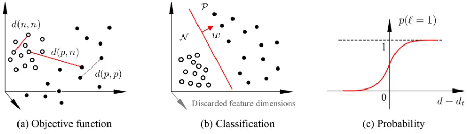
Figure 3: (a) The objective function of sparse descriptor learning. (b) The zero entries in the learnt w remove the salient feature dimensions (region candidates), the non-zero entries define the hyperplane for classification in the salient feature space. (c) The sigmoid probability function.

filters but with enhanced smoothness and complementary properties. We calculate the response map of the image to each filter, and accumulate over the i-th region to obtain the region descriptor Φi ∈ R1×9. The region descriptors from different locations and

pyramid levels form a candidate pool Φ ={Φi}Ni=1 ∈RN

×9_{, where N is the total number}

of the region candidates. Φ gives a redundant (overcomplete) description of the image, see Fig. 1(b).

The task then is to select from the candidate pool Φ a few regions containing the dis-criminative information, which we formulate as a sparse learning problem. The selection can be described by the operation,

φ=W12Φ. (1)

W ∈_RN×N _{is a diagonal matrix with sparse entriesw = [w}

1, w2, . . . , wN], in which wi is

the assigned weight of the i-th region Φi, and the non-zeros weights corresponding to the regions selected. φ represents the selected salient features (Fig. 1(c)).

The objective is to learn w such that the selected descriptors φare consistent within class and discriminative between classes. Let φ(p), p ∈ P and φ(n), n ∈ N be the descriptors of two random examples from the positive and negative image set respectively. The distances between the descriptors can be calculated by,

||φ(p)−φ(n)||2 2=

PN i=1||

√

w_iΦi(p)−

√

w_iΦi(n)||2= PN

i=1wi||Φi(p)−Φi(n)||2=wTd(p, n), (2)

where d(p, n) ∈ _RN×1 _{is a vector with each entry d}

i(p, n) being the feature difference calculated at a region, i.e., di(p, n) =||Φi(p)−Φi(n)||2.

Similarly we randomly sample two examplesn1, n2 ∈ N from the negative set and cal-culate the distance denoted by d(n1, n2). To penalise the differences within the negative set and reward the distances between the positive and negative sets, we set a margin-based constraint,

wTd(n1, n2) + 1<wTd(p, n). (3)

We do not penalise the differences within the positive set as it represents the misaligned or pathological images with large variations, see Fig. 3(a).

The objective function enforcing the constraint may be composed in a sparse learning form,

arg min

w>0

X

p∈P;n,n1,n2∈N

where L(z) = max{z+ 1,0} is a loss function penalising the non-discriminative entries, and the `1-norm ||w||1 is a sparsity-inducing regulariser which encourages the entries of

w to be zero, thus performs region selection. Note that eachn in the function represent an independent random index from the negative set, and p from the positive set. The number of the summands is not fixed, which fits with the stochastic learning and online optimisation procedure, i.e., repetitively drawing random samples d(n1, n2), d(p, n) and optimising w until a criterion is met. The random sampling also enables incremental learning which means we can refine the model without re-learning it all over again when new training data become available. We deduce the solution to (4) in the next section.

2.2

Optimisation

Finding the sparse parameter w in (4) is a regularised stochastic learning problem where the objective function is the sum of two convex terms: one is the loss function of the learning task fed recursively by random examples, and the other is a `1-norm regulari-sation term for promoting sparsity. It can be solved efficiently by the Regularised Dual Averaging (RDA) algorithm [3, 4], which recursively learns and updates w with new examples.

At the t-th iteration, RDA takes in a new observation, which in our case are random pairs d(p, n) andd(n1, n2). The loss subgradient gt is calculated by,

g_t =∂L w

T_(d(n

1, n2)−d(p, n))

∂w

=

(

d(n1, n2)−d(p, n), wT (d(n1, n2)−d(p, n))>−1

0, otherwise.

(5)

g_t is used to update the average subgradient, ¯g_t = 1_tPt

i=1gi. Updating the parameter

w with RDA takes the form,

wt+1 = arg min

w

(wTg¯_t+u||w||1+

βt

t h(w)) (6)

in which the last term is an additional strong convex regularisation term. One can set

h(w) = 1₂||w||2

2 = 12w T_w,β

t=γ

√

t, γ >0 for a convergence rate ofO(1/√t). By writing

u as a N dimension vector with each elements being u, equation (6) becomes,

wt+1 = arg min

w

(wTg¯_t+wTu + γ 2√tw

T_{w), (7)}

which can be solved by Least Squares method to give,

wt+1 =−

√ t

r (¯gt+u). (8)

The discriminative regions and optimal descriptors are obtained by keeping only the candidates with non-zero weights indicated by the learnt w. An example is given in Fig. 1(d).

2.3

Localisation and Classification

Figure 4: Applying the learnt descriptors for localisation and classification.

2.3.1 Localisation.

The anatomy is described discriminatively by φl which represents the salient structures. Localising the anatomy in the image is conducted by searching for these structures. Given an initial estimation x(0) _{of the location, which can be set at the centre of the image,} the descriptor at the initial location φl(x(0)) is observed to deduce the true location x∗. The deduction can be expressed as solving the regression φl(x(0)) 7→ x∗. The direct mapping function is non-linear in nature and training such function comes up against the over-fitting problem. In practice the mapping can be decomposed into a sequence of linear mapping and updating steps,

(

Mapping: φl(x(k))7→∆x(k),

Updating: x(k+1)_=x(k)_{+ ∆x}(k)_, (9)

where in the mapping stage, a prediction for the correction of the location is made, based on the observation φl(x(k)) at the current location x(k); and in the updating stage, the location and observation is updated. The learning mapping function is set to be,

∆x(k)=R(k)φl(x(k)) +b(k), (10)

with R(k) being a projection matrix and b(k) the bias. {R(k),b(k)} in each iteration is trained with the Supervised Descent Method, the details of which can be found in [14].

2.3.2 Classification.

Learningw in the objective function (4) can be viewed as a simultaneous feature selection and classification process. The zero entries in w correspond to the non-salient features (or region candidates) to be discarded. In fact, the non-zero entries in w form a vector defining the hyperplane classifying the positive and negative samples in the salient feature space, which is similar to a support vector in Support Vector Machine classifier, see Fig 3(b).

For a specific pathological condition, the learnt descriptorφccovers the regions where the abnormalities are most likely to appear, and preserves their discriminative features for classification. To predict the class label ` of a test image, we extract the descriptor φc(x∗) at the detected location x∗ and calculate the average distance to the normal descriptors,

d= 1

|N |

X

n∈N

where n indexes all the cases in the normal setN.

A larger d indicates a greater probability of the case being abnormal. More formally, the probability of the case being abnormal is modelled by a sigmoid function (Fig. 3(c)),

p(`= 1|φc(x∗)) =

1

1 +e−(d−dt), (12)

where dt is a threshold distance. The cases with p > 0.5 are classified as abnormal, with confidence p. Conversely, the cases with p < 0.5 are classified as normal with the confidence (1−p).

3

Experiments

3.1

Clinical background

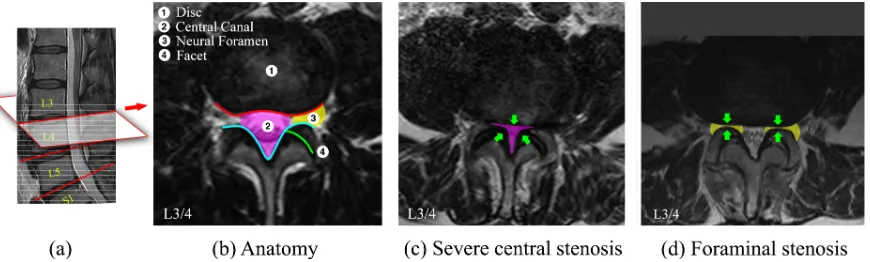
Lumbar spinal stenosis (LSS) is a common disorder of the spine. The disorder can be observed in radiological studies as morphological abnormalities. Intervertebral disc-level axial images in MRI scans can provide rich information revealing the condition of important anatomies such as the disc, central canal, neural foramen and facet. In most cases the original axial scans are not aligned to the disc planes caused by the curvature of the spine. To obtain the precise intervertebral views, we localise the disc planes in the paired sagittal scans (red line in Fig 5), and map the geometry to the axial scans to calculate the coordinates, where the voxels are sampled to extract the aligned images. On a disc-level image shown in Fig. 5(b), conditions of the posterior disc margins (red line) and the posterior spinal canal (cyan line) are typically inspected for the diagnosis. Degeneration of these structures can constrict the spinal canal (pink area) and the neural foramen (yellow area) causing central and foraminal stenosis.

Data. The data collected from routine clinics consists of T2-weighted MRI scans of

600 patients with varied LSS symptoms. Each patient has paired sagittal-axial scans. The L3/4, L4/5, L5/S1 intervertebral planes are localised in the sagittal scans and the images sampled from the axial scans. We obtain three sets of 600 disc-level axial images for the three intervertebral planes respectively. The images are resampled to have an pixel space of 0.5 mm. All cases are inspected and annotated with classification labels with respect to the central stenosis and foraminal narrowing. In addition, the dense annotations are available for the first 192, 198, 192 images in the three subsets, in which each image is delineated with 37 landmarks outlining the disc, central canal and facet, see Fig. 7(a). In summary the dataset for validation contains three sets of 600 data with classification labels and three subsets of 192, 198, 192 data with dense annotations, which are referred to as weakly and densely annotated datasets respectively.

3.2

Results

3.2.1 Validation protocols.

Figure 5: (a) Mid-sagittal view of a lumbar spine. Grey dashed lines show the raw axial scans. Red lines show the aligned disc-level planes, from which the axial images are extracted. (b) Anatomy of a L3/4 disc-level axial image. (c) A case with severe central stenosis. (d) A case with foraminal stenosis

and task-specific classifications. In the testing stage, the localisation and classification tasks are carried out by each method independently, and the performance is evaluated.

3.2.2 Anatomy localisation.

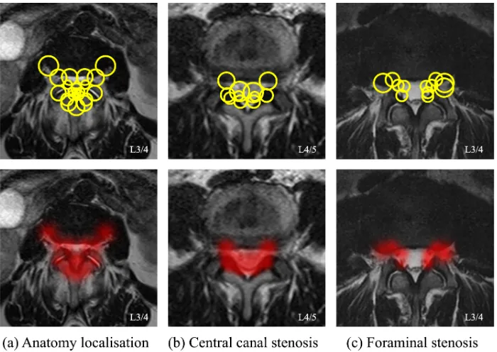
The learning result of the optimal descriptor for localising the vertebrae, L3/4 as an example, is shown in Fig. 6(a). The hot maps of salient regions are visualised by showing the selected region candidates as Gaussian blobs. It is interesting to compare these with the biological anatomy in Fig. 5(b) and the annotations by the clinician in Fig. 7(a). The learnt descriptor highlights the posterior margin of the disc and the posterior arch, which have sharp textures and high contrast. Note that compared with a clinician’s annotations, the front edge of the disc is not selected. The reason for this may be there being less consistency across images because of the variation in disc size, as well as the ambiguous boundaries to the abdominal structures in some of the cases.

We compare our method with HOG grid [6] and Deformable Part Models (DPM) [7, 15]. The HOG grid is a hand-crafted descriptor covering the holistic appearance, see Fig. 7(b). It assumes no prior clinical knowledge and assigns equal weights to the local features of the anatomy. The DPM is a strongly supervised method which describes the anatomy by local patches at each of the landmarks as well as the geometry of the landmark locations (Fig. 7(c)). Each patch is described by a SIFT descriptor. In all the methods the initial location is set at the centre of the images and the searching is driven by the SDM algorithm [14]. The experimental results are reported in Table 1. The initial distances to the true locations are also given. We can see that our learnt descriptors give comparable localisation precision with DPM when trained on the same densely annotated subsets, but use no landmark annotation. With further training on additional data, a significant improvement is observed indicating the learning ability of our method on weakly annotated data.

3.2.3 Pathology classification.

Figure 6: The discriminative descriptors (top) and evidence regions (bottom) learnt for the task of (a) anatomy localisation (b) central stenosis classification and (c) foraminal stenosis classification.

Figure 7: Comparative descriptors: landmarks, HOG-grid and DPM.

Table 1: Precision of anatomy localisation in mm (+ _{Require landmarks. * Trained on} additional weakly annotated data).

Data Initial HOG grid∗ _DPM+ _{Learnt Learnt*}

L3/4 16.41±10.10 2.45±1.69 2.01±1.62 1.95±1.58 1.22±1.01 L4/5 16.59±10.80 2.37±1.55 1.73±1.30 1.76±1.26 1.57±1.36 L5/S1 12.86±8.29 2.52±1.71 1.85±1.42 2.09±1.52 1.24±0.96

labels, it pinpoints the neural foramen as the evidence regions. These evidence regions pinpointed automatically by our methods (Fig. 6(b)(c)) show high agreement with the medical definition of the pathologies shown in Fig. 5(c)(d).

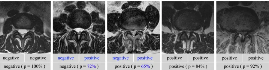
Figure 8: Example images with different degrees of degeneration. First row: the repeated labels for central stenosis by the same clinician, made at different times. Disagreement is shown in blue. Second row: the labels and probabilities by our classification method. Table 2: Agreement (%) of classification. (+_{Require landmarks. * Trained on additional} weakly annotated data.)

Human HOG grid DPM(Geo)+ _DPM(SIFT)+ _{Learnt Learnt*}

Central canal stenosis

L3/4 88.5 80.6±4.9 79.5±4.5 81.0±4.9 85.7±3.5 87.2±3.2

L4/5 87.4 81.3±4.6 78.3±4.1 82.4±4.5 84.2±3.4 85.1±3.4

L5/S1 89.2 81.8±4.7 81.4±4.5 82.7±4.4 86.0±3.7 87.5±3.3

Foraminal stenosis

L3/4 86.5 79.6±4.5 81.2±4.8 83.1±4.7 82.9±4.5 84.3±3.9

L4/5 87.2 81.5±4.9 82.4±4.6 83.3±4.3 82.5±4.5 84.0±4.0

L5/S1 89.5 81.7±4.4 81.8±4.7 82.9±4.5 84.1±3.8 87.1±3.4

as the weak learners. The performance is evaluated by the agreement with labelling done by a clinician, calculated by (pp+nn)/M, in whichpp and nnare the number of agreed positive and agreed negative cases, and M is the total number of cases.

The results of the two classification tasks are shown in Table. 2. Our descriptor learn-ing method gives better or competitive classification accuracies compared with supervised methods, trained on the same densely annotated subset but requires no landmarks to be identified. A significant improvement is again seen with additional training on weakly annotated data. Note that the performance is affected by the precision of the human labels, as the clinician can only achieve a certain level of agreement between themselves when the labelling step is repeated on same dataset. We report the self-agreement of a clinician in Table. 2, denoted as the human performance. The disagreement is generally caused by ambiguous conditions in many cases. We give several example images with different degrees of degenerations, and show the classification labels by the clinician as well as the labels and probabilities by our method in Fig. 8. The probability indicates the confidence of our prediction, which may be helpful for being aware of and understanding errors in the classification results.

4

Conclusions

straightfor-ward with no need of parameter tuning. We have shown that promising results can be achieved when learnt on 600 labelled images. The average training time for one task is about 27 minutes in MATLAB on a 3.20 GHz GPU with 16 GB RAM. The method can be readily applied to other clinical tasks for rapidly pinpointing and describing evidence of abnormalities directly from expertly labelled data. Further work includes extending the method to 3D where the increased scale might be handled by random candidate sam-pling. The MATLAB toolbox of the methods described here will be made public available for research purposes.

References

[1] Simonyan, K., Vedaldi, A., Zisserman, A.: Descriptor learning using convex optimi-sation. In: European Conference on Computer Vision, Springer (2012) 243–256

[2] Simonyan, K., Vedaldi, A., Zisserman, A.: Learning local feature descriptors using convex optimisation. IEEE Transactions on PAMI36(8) (2014) 1573–1585

[3] Xiao, L.: Dual Averaging Method for Regularized Stochastic Learning and Online Optimization. In: Advances in Neural Information Processing Systems. Curran Associates, Inc. (2009) 2116–2124

[4] Xiao, L.: Dual averaging methods for regularized stochastic learning and online optimization. Journal of Machine Learning Research 11(Oct) (2010) 2543–2596

[5] Chen, Y., Bi, J., Wang, J.Z.: Miles: Multiple-instance learning via embedded instance selection. IEEE Transactions on PAMI 28(12) (2006) 1931–1947

[6] Lootus, M., Kadir, T., Zisserman, A.: Vertebrae detection and labelling in lumbar MR images. In: MICCAI CSI Workshop. Springer (2013) 219–230

[7] Zhao, Q., Okada, K., Rosenbaum, K., Kehoe, L., Zand, D.J., Sze, R., Summar, M., Linguraru, M.G.: Digital facial dysmorphology for genetic screening: hierarchical constrained local model using ICA. Medical Image Analysis 18(5) (2014) 699–710

[8] Shen, W., Zhou, M., Yang, F., Yang, C., Tian, J.: Multi-scale convolutional neu-ral networks for lung nodule classification. In: International Conference on IPMI, Springer (2015) 588–599

[9] Shin, H.C., Roth, H.R., Gao, M., Lu, L., Xu, Z., Nogues, I., Yao, J., Mollura, D., Summers, R.M.: Deep convolutional neural networks for computer-aided detection: CNN architectures, dataset characteristics and transfer learning. IEEE Transactions on Medical Imaging 35(5) (2016) 1285–1298

[10] Schlegl, T., Waldstein, S.M., Vogl, W.D., Schmidt-Erfurth, U., Langs, G.: Predicting semantic descriptions from medical images with convolutional neural networks. In: International Conference on IPMI, Springer (2015) 437–448

[12] Oquab, M., Bottou, L., Laptev, I., Sivic, J.: Is object localization for free? Weakly supervised learning with convolutional neural networks. In: Proceedings of the IEEE Conference on CVPR. (2015) 685–694

[13] Jamaludin, A., Kadir, T., Zisserman, A.: SpineNet: Automatically Pinpointing Classification Evidence in Spinal MRIs. In: International Conference on MICCAI, Springer (2016) 166–175

[14] Xiong, X., Torre, F.: Supervised descent method and its applications to face align-ment. In: Proceedings of the IEEE conference on CVPR. (2013) 532–539