http://wrap.warwick.ac.uk
Original citation:
Franzke, Christian L. E., Osprey, Scott M., Davini, Paolo and Watkins, Nicholas W..
(2015) A dynamical systems explanation of the Hurst effect and atmospheric
low-frequency variability. Scientific Reports, Volume 5 . Article number 9068. ISSN
2045-2322
Permanent WRAP url:
http://wrap.warwick.ac.uk/66942
Copyright and reuse:
The Warwick Research Archive Portal (WRAP) makes this work of researchers of the
University of Warwick available open access under the following conditions.
This article is made available under the Creative Commons Attribution 4.0 International
license (CC BY 4.0) and may be reused according to the conditions of the license. For
more details see:
http://creativecommons.org/licenses/by/4.0/
A note on versions:
The version presented in WRAP is the published version, or, version of record, and may
be cited as it appears here.
A Dynamical Systems Explanation of the
Hurst Effect and Atmospheric
Low-Frequency Variability
Christian L. E. Franzke1, Scott M. Osprey2, Paolo Davini3& Nicholas W. Watkins4,5,6,7
1Meteorological Institute and Center for Earth System Research and Sustainability (CEN), University of Hamburg, Hamburg,
Germany,2National Centre for Atmospheric Science and Department of Physics, University of Oxford, Oxford, UK,3Institute of
Atmospheric Sciences and Climate (ISAC-CNR), Torino, Italy,4Max-Planck Institute for the Physics of Complex Systems, Dresden,
Germany,5Centre for the Analysis of Time Series, LSE, London, UK,6MCT, Open University, Milton Keynes, UK,7CFSA, University of
Warwick, Coventry, UK.
The Hurst effect plays an important role in many areas such as physics, climate and finance. It describes the anomalous growth of range and constrains the behavior and predictability of these systems. The Hurst effect is frequently taken to be synonymous with Long-Range Dependence (LRD) and is typically assumed to be produced by a stationary stochastic process which has infinite memory. However, infinite memory appears to be at odds with the Markovian nature of most physical laws while the stationarity assumption lacks robustness. Here we use Lorenz’s paradigmatic chaotic model to show that regime behavior can also cause the Hurst effect. By giving an alternative, parsimonious, explanation using nonstationary Markovian dynamics, our results question the common belief that the Hurst effect necessarily implies a stationary infinite memory process. We also demonstrate that our results can explain atmospheric variability without the infinite memory previously thought necessary and are consistent with climate model simulations.
H
urst’s environmetric observations in the 1950s first sparked interest in the natural phenomenon ofanomalously fast growth of rescaled range in hydrological time series, most famously from the Nile river1,2.
Rescaled range is a measure of the variability of a time series and is calculated by dividing the range of the values by the standard deviation. This is done for increasing window sizes which are than averaged2,3.
These observations of the growth of range of what is now known as the ‘Hurst’ effect stimulated much debate, because Feller showed rigorously that for a very general class of finite variance stochastic processes, the rescaled range grows asymptotically with the record lengthLasL1/2 4. Many explanations centered on pre-asymptotic
effects, but a more mathematically elegant explanation came with the introduction by Mandelbrot, Van Ness and Wallis of fractional Gaussian noise (fGn), the first stationary model which was able to reproduce them. fGn was in itself controversial, however5,6, because it gained the desirable and tractable property of stationarity at the price of
introducing infinite-ranged temporal memory or LRD. LRD implies that in order to predict the next state of a system its whole past is needed. This is different from typical dynamical systems whose next state is determined just by the current state. Such systems are called Markovian. This property appeared to many to be inconsistent with the Markovian nature of the equations of motion.
However Mandelbrot, as early as 19655,7and contemporary with his work on fGn and fractional Brownian
motion (fBm), showed that at least one other type of non-stationary model could exhibit the Hurst effect. This other model has not received the same attention as stationary LRD models and raises an important question of what should be used for the modeling of natural systems. To the relatively familiar random walk models such as his own fBm, which is integrated fGn, Mandelbrot added a class of switching models with long tailed distributions for the intervals between the state changes, which he called ‘‘conditionally stationary’’. Stationary fGn and these two classes of non-stationary models all shared a form of 1/f power spectrum at low frequencies, the signature of self-affinity. The presence of fluctuations on all timescales in 1/f noises complicates inference of trends in short time series, as seen for instance in climate8–10and hydrology11. Whether a complex system such as the climate is
stationary or non-stationary, and if the latter, what type, thus has significant implications for our ability to perform skillful predictions. However, the very ubiquity of 1/f noise poses a problem, in Mandelbrot’s own words that‘‘reducing the notion of 1/f noise’’ to ‘‘self-affinity … shows it to be very severely under-specified’’6, so that other
considerations need to be taken into account when choosing a model.
SUBJECT AREAS:
NONLINEAR PHENOMENA
ATMOSPHERIC DYNAMICS
Received 30 November 2014
Accepted 12 February 2015
Published 13 March 2015
Much empirical model choice has been based on the idea of par-simony (Occam’s razor), a principle of model selection which states that one should select the model with the fewest necessary assump-tions. Parsimony favors ‘‘simplicity’’ or ‘‘elegance’’, but these con-cepts admit different interpretations in different sciences. A more complicated model can turn out to be more skillful12, but this skill
may be at the expense of insight. In the end, however, whether a complex system is better described by a stationary or non-stationary model may not be decided purely by parsimony. In geosciences physical reservations about the LRD concept, and an apparent lack of awareness that Mandelbrot had already proposed a conditionally stationary alternative7, motivated Klemes13 to discuss switching
models, while Bhattacharya et al.14 showed that the presence of
trends could produce a Hurst effect under certain conditions. However in econometrics, it has long been recognized by some authors that in addition to the classes of models discussed above, it is essential to consider alternatives which are motivated by parsimo-nious assumptions about the time series. In particular, Diebold and Inoue15have shown that some Markovian regime switching models
can indeed produce 1/f signatures over a wide frequency range, des-pite not possessing long tailed distributions of times between switch-ing, and have argued that they may be more relevant in some systems. Mesa et al.16have argued on physical grounds for the importance of
deterministic low dimensional chaos as an origin for the Hurst effect, in particular focusing on the ‘critically slowed’ motion in systems close to a bifurcation.
It is well known that LRD requires slow, algebraic decay of the empirical autocorrelation function;r(t),t2d21 17,18, but,
impor-tantly, it also assumes stationarity17, without which a memory
extending tot5 2‘cannot be defined. When it is observed, the Hurst phenomenon is usually attributed to phenomena which are best described by stochastic processes, such as: self-similar scaling processes, aggregation of short-range dependent stochastic pro-cesses, turbulence or the distributional properties of waiting times (see Refs. 7, 17 for more details). The memory parameterdis
con-ventionally defined17via the slope of the power spectrum, or
alter-natively by the slope of the decay of the autocorrelation function, on a doubly logarithmic plot. For d.0 we talk about persistent time series, where large values tend to be followed by large values and vice versa. For d,0 we have anti-persistence; i.e. positive values tend to be followed by negative values and vice versa. For d50 we have white noise; i.e. no autocorrelation. The widely used autoregressive models approach a white noise power spectrum for large time scales8.
Here we show that one of the most seminal models of determin-istic chaotic dynamics, Lorenz’s 1963 model19which he abstracted
from Rayleigh-Benard convection, exhibits the Hurst effect. We show that the origin of the Hurst effect in the Lorenz model is regime behavior. This has implications for our understanding of how the Hurst effect can arise, and for how we interpret observational data in many fields. That the Lorenz 63 model exhibits the Hurst effect is a surprising and counter-intuitive result because deterministic chaotic systems are frequently thought to be white noise on time scales larger than the Lyapunov time scale (e.g. Ref. 20), and they are sometimes used for the generation of independent and identically distributed (iid) random numbers21.
The Paradigmatic Model: Lorenz 63
The nonlinear deterministic Lorenz 63 model19is given by:
dx
dt~sðy{xÞ ð1Þ
dx
dt~x rð {zÞ{y ð2Þ
dz
dt~xy{bz: ð3Þ
It is the archetypal model for deterministic chaos19. We use the
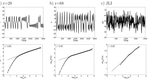
[image:3.595.51.552.47.316.2]standard parameter values,b58/3 ands510 and varyr. Fig. 1a shows the typical behavior of the standard Lorenz model withr528.
Figure 1| Time series (upper row) and DFA2 (lower row) for a) the Lorenz 63 model with r528, b) the Lorenz 63 model with r568 and c) the JLI derived from ERA40 reanalysis data36. The regression line is trending upward towards lower frequencies for the r528 case and the JLI with a slope larger than 0.5 whereas the slope is about 0.5 for the r568 case. These results are consistent with the r528 case and the JLI exhibiting the Hurst effect and the r568 case being white noise. The time series is sampled in 0.1 time units.
With these settings the system stays for relatively long periods within one wing of the attractor before eventually switching to the other wing, thus, exhibiting persistent regime behavior. However, as we increaserthe regime behavior survives but becomes less persistent. By increasingrboth attractor wings are still present but the trajectory switches more frequently between them (Fig. 1b).
Analyzing the Lorenz 63 model by increasingrshows the impact of the regime behavior on the Hurst effect. For measuring the Hurst effect we have employed several methods: power spectral methods17
and Detrended Fluctuation Analysis (DFA, see Methods and
Data)22,23. For computing DFA we use quadratic polynomial
detrending (referred to as DFA2). Our results are insensitive to the order of the detrending.
We find that the standard case (r528) exhibits the Hurst effect
with a Hurst exponent of H~dz1
2~0:65. The DFA2 scaling extends over almost 4 orders of magnitude with no sign of leveling
off of the scaling on the longest timescales. This provides strong evidence for the Hurst effect in the Lorenz 63 model (Fig. 1).
DFA2 shows that experiments withrlarger than 58 are however consistent with scaling expected from white noise (Fig. 1). Here we argue that the reduction in the magnitude of the Hurst exponent arises likely from the time the Lorenz 63 model resides continuously in one of the two regime states as shown in Fig. 2. This figure displays the complementary cumulative distribution of the residence time, i.e. of the length of the periods the system spends in one of the two regime states. This figure shows that for increasingrthe residence time progressively decreases.
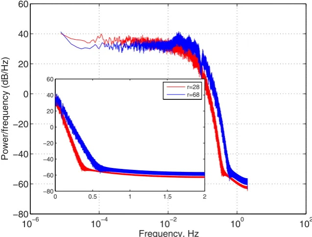
To further check whether the Lorenz 63 model shows the Hurst effect we computed the power spectrum using the Welch period-ogram method (see Methods and Data). The inset of Fig. 3 shows for high frequencies the exponential form for the periodogram reported by several previous authors24–26. However, in the main
plot of Fig. 3 we can see that in the r 5 68 case the power
spectrum becomes flat for low frequencies and is thus consistent with white noise and inconsistent with a Hurst effect, whereas for
r528 an upward trend towards the lowest frequencies is clearly seen, consistent with the Hurst effect reported by DFA. We get similar results when using the GPH estimator (see Methods and Data)27.
As shown in Fig. 2 the residence time decays exponentially. This indicates a memory-less switching process between the two regime states in the Lorenz 63 model consistent with the study by Aizawa28.
Such a process has a mean regime residence timetResin one of the
attractor wings (Tab. 1). This residence time is significantly longer than the Lyapunov time scale. It is frequently assumed that the Lyapunov time scale determines the limit of predictability, and that beyond these time scales systems are effectively characterized by white noise; i.e. are not predictable. The largest Lyapunov exponent provides an estimate for the rate of separation of two trajectories which are initially infinitesimally close to each other. We find that the time scale associated with the largest Lyapunov exponent of the Lorenz 63 model is significantly shorter than the time scales over which we find the Hurst effect occurring (i.e.tL,tRes(Tab. 1)). This
challenges the idea that deterministic chaotic systems are necessarily unpredictable on time scales much longer than the Lyapunov time
500 1000 1500 2000 2500 3000
10−4 10−2 100
Residence Time
1−CDF
[image:4.595.58.281.51.228.2]R=28 R=38 R=48 R=58 R=68 R=78
Figure 2|Cumulative distribution functions of the residence time for the Lorenz 63 model for various values of the r parameter.The residence time is measured in 0.1 time units.
10−6 10−4 10−2 100 102 −80
−60 −40 −20 0 20 40 60
Frequency, Hz
Power/frequency (dB/Hz)
0 0.5 1 1.5 2
−80 −60 −40 −20 0 20 40 60
r=28 r=68
[image:4.595.138.457.476.718.2]scaletL. Our results are consistent with the idea that the
predictabil-ity of multi-scale systems can be enhanced beyond the Lyapunov time scale20. Our results provide evidence that the Lorenz 63 model
can be seen as a system with multiple or a continuum of time scales and has not just one intrinsic time scale. The multiple time scales are due to the chaotic regime switching which occurs randomly.
As with all time series analysis our results come with the caveat of finite size effects. While we cannot rule out that on much longer time scales the slope will eventually approach 0.5, i.e. iid white noise, we find strong evidence for the Hurst effect in the Lorenz 63 model because the scaling extends over 4 orders of magnitude, and is con-firmed by spectral analysis. Furthermore, our time series lengths are comparable with the lengths of many observed natural time series. Thus, our results clearly apply to the interpretation of observed time series. The growth of range on these long time scales due to regime behavior causes significant impacts on predictability, extremes and trends29,30.
The Hurst Effect in the Atmosphere
We have shown that the deterministic chaotic Lorenz 63 model exhibits the Hurst effect, and that the regime behavior is its cause. Similar regime behavior exists in the atmosphere and we assert that this is key for explaining the Hurst effect in the atmosphere. The basic idea of this stems from econometrics15. Diebold and Inoue15showed
both theoretically and by Monte Carlo simulations that
Markov-switching models are able to produce the Hurst effect when the corresponding Markov transition matrix is metastable31. This
corre-sponds to persistent regime behavior where the system stays close to one region in phase space before it eventually switches to another region to stay in that region for a long period. Such a behavior is ubiquitous in the atmosphere32–35.
To identify the presence of the Hurst effect in the atmosphere, we analyze the North Atlantic jet stream in both reanalysis and climate model simulations (see Methods and Data), whose variations greatly impact European climate. We use the Jet Latitude Index (JLI) as a measure of the North Atlantic jet stream36. In Franzke30it has been
argued that the regime behavior of the JLI is responsible for the Hurst effect of surface wind speeds. Here we show evidence that even the JLI exhibits the Hurst effect (Fig. 1c). The JLI shows scaling over up to two order of magnitude. The JLI has a Hurst exponent ofH50.59 in the reanalysis data. Franzke et al.35showed that the regime behavior
is consistent with an eddy-mean flow feedback due to wave breaking. Thus, this nonlinear deterministic behavior is intimately associated with the Hurst effect. This provides a new physical mechanism for explaining the Hurst effect in the atmosphere, which has hitherto been lacking.
A fact which hasn’t been widely appreciated is that persistent jet states are self-maintaining37. This self-maintenance arises from
eddy-mean flow feedbacks and Rossby wave breaking, which are fundamental properties of geophysical flows. Hence, regime beha-vior and the Hurst effect are intrinsic properties of geophysical flows and the atmosphere. Hence, it is important that climate models capture this phenomenon in order for us to have confidence in their ability to predict future climate.
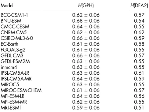
We now evaluate whether the current generation of climate mod-els (see Methods and Data) reproduce the Hurst effect characteristics of the observed JLI in reanalysis data. For this we use the historical simulations from the CMIP5 archive38. As Fig. 4 shows, most CMIP5
models exhibit the Hurst effect with roughly the right magnitude (Tab. 2). Most CMIP5 models show scaling over up to two orders of magnitude. While the CMIP5 models don’t capture the shape of the observed JLI PDF39they still seem to capture the essential
[image:5.595.44.291.94.181.2]atmo-spheric dynamics of the jet stream. Recent studies show that very high resolutions are needed to accurately reproduce the geographical
Table 1 | Hurst exponent (H(DFA), Lyapunov time (tL) and mean
regime residence time (tRes) of the x-component of Lorenz 63
model for various values of the Rayleigh parameter r
R H(DFA) tL tRes
28 0.65 1.09 19.0
38 0.62 0.91 15.4
48 0.56 0.81 12.5
58 0.50 0.74 10.9
68 0.49 0.68 9.1
78 0.48 0.65 8.7
88 0.49 0.65 6.6
0
1
2
3
4
−0.5
0
0.5
1
1.5
2
2.5
3
log
10
(s)
log
10
(F(s))
JLI slope bcc−csm1−1 BNU−ESM CMCC−CESM CNRM−CM5 CSIRO−Mk3−6−0 EC−Earth FGOALS−g2 GFDL−CM3 GFDL−ESM2M inmcm4 IPSL−CM5A−LR IPSL−CM5A−MR MIROC5
[image:5.595.139.460.476.725.2]MIROC−ESM−CHEM MPI−ESM−LR MPI−ESM−MR MRI−ESM1
Figure 4|DFA spectra of CMIP5 JLIs.The JLI time series are sampled daily.
structure of the atmospheric flow regimes34. However, the CMIP5
models already capture the important geophysical dynamics and, thus, the scaling behavior.
Discussion
Our results clearly show that the Hurst effect is not necessarily syn-onymous with stationary LRD. We showed that a deterministic cha-otic system, the Lorenz 63 model, can exhibit the Hurst effect due to its non-stationary regime behavior. This regime behavior can also be seen as a kind of intermittency which can also create power laws40.
Because the residence time decays exponentially and not like a power law this questions whether the Lorenz 63 model has infinite memory. Typically, systems exhibiting LRD have power-law distributed wait-ing times. This interpretation of our results is consistent with
pre-vious studies15 who have shown that Markov switching models
(which have regime behavior) or more general non-stationary mod-els13produce growth of range without infinite memory, at least over
large ranges of scale.
Many climate scientists are deeply sceptical about LRD on theor-etical grounds41,42, and have transferred this scepticism to the Hurst
effect in the belief that it necessarily corresponds to an infinite mem-ory process. But our results show that in a climate-relevant dynam-ical system, the Hurst effect can arise from well understood nonlinear dynamics.
The wider implications of our results are that regime behavior impacts on trend analysis because the switching can cause apparent trends by e.g. staying in the first half of the time series in one regime state and then switching to another regime state for the second half (see Fig. 1b of Ref. 29 for an illustration of this effect). Furthermore, we showed that the Hurst effect can be an intrinsic property of non-linear dynamical systems. Our ideas put forward here are consistent with the work by Ed Lorenz on climate as an almost intransitive system43. His work suggests that even deterministic systems, when
they are nonlinear, can exhibit variability on very long time scales. Our results on the Hurst effect in climate are consistent with his ideas.
Moreover, our results have implications for future climate projec-tions. We show that on long (but finite) timescales, the Lorenz 63 system exhibits the Hurst effect for lower Raleigh parameter values; physically this denotes a reduced temperature difference between plates in a Rayleigh-Benard experiment. We see in Lorenz 63 that if we make the system less chaotic, the trajectory stays in a given wing
for longer with only inter-mittent sojourns to the other wing. From these results we can make an analogy with the weather conditions affecting Europe and the US in the last few years. We expect a reduced meridional temperature gradient due to declining sea ice extent. We anticipate that this ought to make the (lower) atmosphere more stable (less chaotic) to baroclinic instability. In a system which has regimes this can be seen by greater residence times for a given regime. Many of the recent extreme weather conditions can be linked to unusual and persistent deviations of the jet stream44, though their
significance and relevance has been questioned45. Our results suggest
that the Hurst effect characteristics of the atmosphere might be more important in explaining current extreme weather conditions than previously thought.
Methods
In this study we use data from climate models which has also been used for the latest, Fifth Assessment Report (AR5) of the Intergovernmental Panel on Climate Change (IPCC). The data are from the Coupled Model Intercomparison Project - Phase 5 (CMIP5) which includes a variety of different standardized experiments performed with state-of-the-art general circulation models38. According to the availability on the
online archive (http://pcmdi3.llnl.gov/esgcet/home.htm), historical runs for 25 different climate models spanning over the 1951–2005 period (55 full years) were analyzed. The ensemble member r1i1p1 has been selected for all models included except for the Community Climate System Model (CCSM4; simulation r6i1p1) and the European Centre Earth System Model (EC-EARTH; simulation r8i1p1). The list of the models chosen is shown in Tab. 2. See Ref. 38 for more details about the climate model simulations. We use data from the following modelling groups: Beijing Climate Center (China, BCC-CSM1-1), Beijing Normal University (China, BNU-ESM), Centro Euro-Mediterraneo sui Cambiamenti Climatici (Italy, CMCC-CESM), Meteo-France (France, CNRM-CM5), Commonwealth Scientific and Industrial Research Organisation (Auistralia, CSIRO-Mk3-6-0), European Network for Earth System Modelling (EC-EARTH), State Key Laboratory Numerical Modeling for atmospheric Sciences and geophysical fluid Dynamics (China, FGOALS-g2), Geophysical Fluid Dynamics Laboratory (USA, GFDL-CM3 and GFDL-ESM2M), Russian Academy of Sciences Institute of Numerical mathematics (Russia, inmcm4), Institut Pierre Simon Laplace (France, IPSL-CM5A-LR and IPSL-CM5A-MR), International Centre for Earth Simulation (Japan, MIROC5 and MIROCESM-CHEM), Max-Planck Institute for Meteorology (Germany, ESM-LR and MPI-ESM-MR) and Meteorological Research Institute (Japan, MRI-ESM1). More information about the CMIP5 climate models and the data can be found at: http:// esgf-data.dkrz.de/esgf-web-fe/.
The Jet Latitude Index (JLI)36is introduced in order to describe the daily variability
of the latitudinal position of the eddy-driven Atlantic jet stream. The JLI is defined as the latitude of the zonally averaged maximum of the zonal wind speed between 60uW and 0uW longitude at 850 hPa. A 5-day running-mean is applied in order to exclude synoptic variability. Model data are interpolated on the 2.5u32.5ugrid using a second order conservative remapping algorithm. Only values between 15uN and 75uN are retained to avoid orographic effects. The CMIP5 JLI index is slightly differently defined from Woollings et al.36but both versions are highly correlated. Furthermore,
also a JLI derived from the 20th Century National Center for Environment Prediction (20C NCEP) reanalysis data show very similar results to the European Centre for Medium-Range Weather Forecasts ERA40 JLI results. This provides further evidence that our results are robust.
In order to examine the Hurst effect we use DFA8,22,41,46. In DFA, first a profile
Y ið Þ~XN
t~1x tð Þis computed. This profile is then split up intoNsnon-overlapping
segments of equal length s. After that the local trend is subtracted for each segment v by a polynomial least-squares fit of the data. Linear (DFA1), quadratic (DFA2), cubic (DFA3) or higher-order polynomials can be used for detrending. In the nth-order DFA, trends of order n in the profile, and of order n-1 in the original record, are eliminated. Next, the variance for each of theNssegments is calculated by averaging
over all data points i in the v-th segment:
F2
s~vYs2ð Þiw~
1 2
Xs
i~1
Y2
s½ðv{1Þsi ð4Þ
Finally, the average over all segments is computed and the square root is applied to obtain the following fluctuation function:
F sð Þ~
ffiffiffiffiffiffiffiffiffiffiffiffiffiffiffiffiffiffiffiffiffiffiffiffi
1
Ns
XNs
v~1
F2
sð Þv v
u u
t ð5Þ
For different detrending orders, n, we obtain different fluctuation functions F (s), which are denoted byF(n),(s). The fluctuation function scales according to
[image:6.595.45.290.103.286.2]F(n)(s),sf, withfcorresponding to the Hurst exponent H andd~f{1 2. We also use the Welch method to estimate the spectral density of the time series. This method reduces the variance of the periodogram by splitting the time series into
Table 2 | Hurst exponent H values of JLI from CMIP5 historical forcing runs covering the period 1951 through 2005. Hurst expo-nents have been computed by the GPH and DFA2 estimators. The GPH estimator also provides the 5% confidence levels
Model H(GPH) H(DFA2)
BCC-CSM1-1 0.6260.06 0.57
BNU-ESM 0.6860.06 0.54
CMCC-CESM 0.6460.06 0.55
CNRM-CM5 0.6260.06 0.62
CSIRO-Mk3-6-0 0.6660.06 0.59
EC-Earth 0.6160.06 0.58
FGOALS-g2 0.6160.06 0.55
GFDL-CM3 0.6660.06 0.57
GFDL-ESM2M 0.6360.06 0.55
inmcm4 0.6360.06 0.55
IPSL-CM5A-LR 0.6360.06 0.61
IPSL-CM5A-MR 0.6460.06 0.59
MIROC5 0.6360.06 0.55
MIROC-ESM-CHEM 0.6160.06 0.57
MPI-ESM-LR 0.6460.06 0.56
MPI-ESM-MR 0.6260.06 0.55
overlapping segments. For each segment the periodogram is computed and these estimates are averaged.
Furthermore, we use also a power spectral estimator to infer the Hurst exponent. In particular, we are using the GPH estimator27,46. This estimatior finds the Hurst
exponent by estimating the spectral slope using the periodogram.
1. Hurst, H. E. Long-term storage capacity of reservoirs.Amer. Soc. Civil Eng. Trans. 116, 770–808 (1951).
2. Hurst, H. E. A suggested statistical model of some time series which occur in nature.Nature,180, 494 (1957).
3. Feder, J.Fractals, 1st ed., 305p. (Springer, 1988).
4. Feller, W. The Asymptotic Distribution of the Range of Sums of Independent
Random Variables.Ann. Math. Stat.22, 427–432 (1951).
5. Graves, T., Gramacy, R. G., Watkins, N. W. & Franzke, C. L. E. A brief history of
long memory.Am. Stat.submitted. arxiv:1406.6018.
6. Mandelbrot, B. B. inMultifractals and 1/f noise: Wild Self-Affinity in Physics.1st ed., 442p. (Springer 1999).
7. Mandelbrot, B. B. Some noises with 1/f spectrum, a bridge between direct current and white noise.IEEE Trans. Inf. Theory,IT–13, 289–298 (1967).
8. Bunde, A., Ludescher, J., Franzke, C. L. E. & Bu¨ntgen, U. How significant is West Antarctic warming?Nature Geoscience,7, 246–247 (2014).
9. Franzke, C. Long-range Dependence and Climate Noise Characteristics of Antarctic Temperature Data.J. Climate,23, 6074–6081 (2010). doi: 10.1175/ 2010JCLI3654.1.
10. Franzke, C. Nonlinear trends, long-range dependence and climate noise properties of surface air temperature.J. Climate.25, 4172–4183 (2011). 11. Koutsoyiannis, D. Climate change, the Hurst phenomenon, hydrological
statistics.Hydrol. Sci.48, 3–24 (2003).
12. Zhang, B.-T. & Mu¨hlenbein, H. Balancing accuracy and parsimony in genetic
programming.Evol. Comput.3, 17–38 (1995).
13. Klemes, V. The Hurst phenomenon: a puzzle?Water Resour. Res.10, 675–688
(1974).
14. Bhattacharya, R. N., Gupta, V. K. & Waymire, E. The Hurst effect under trends.
J. Appl. Probab.20, 649–662 (1983).
15. Diebold, F. X. & Inoue, A. Long memory and regime switching.J. Econom.105, 131–159 (2001).
16. Mesa, O., Gupta, V. K. & O’Connell, P. E. inExtreme Events and Natural Hazards:
The Complexity Perspective 1stedn(eds Surjalal Sharma, A.et al.) 209–229
(American Geophysical Union, 2013).
17. Beran, J., Feng, Y., Gosh, S. & Kulik, R.Long-Memory Processes.884p. (Springer, 2013).
18. Makse, H. A., Havlin, S., Schwartz, M. & Stanley, H. E. Method for generating long-range correlations for large systems.Phys. Rev. E,53, 5445 (1996). 19. Lorenz, E. N. Deterministic Nonperiodic Flow.J. Atmos. Sci.20, 130–141 (1963). 20. Boffetta, G., Giuliana, P., Paladin, G. & Vulpiani, A. An Extension of the Lyapunov
Analysis for the Predictability Problem.J. Atmos. Sci.55, 3409–3416 (1998). 21. Szczepaski, J. & Kotulski, Z. Pseudorandom number generators based on chaotic
dynamical systems.Open Syst. Inf. Dyn.8, 137–146 (2001).
22. Koscielny-Bunde, E.et al. Indication of a universal persistence law governing atmospheric variability.Phys. Rev. Lett.81, 729–732 (1998).
23. Peng, C.-K.et al. Mosaic organization of DNA nucleotides.Phys. Rev. E.49, 1685–1689 (1994).
24. Broomhead, G. & King, G. P. Extracting qualitative dynamics from experimental data.Physica D,20, 17–236 (1986).
25. Farmer, D., Crutchfield, J., Froehling, H., Packard, N. & Shaw, R. Power spectra and mixing properties of strange attractors.Annals of the New York Academy of
Sciences.357, 453–471 (1980).
26. Osprey, S. M. & Ambaum, M. H. Evidence for the chaotic origin of Northern Annular Mode variability.Geophys. Res. Lett.38(2011).
27. Geweke, J. & Porter-Hudak, S. The estimation and application of long memory time series models.J. Time Ser. Anal.4, 221–238 (1983).
28. Aizawa, Y. Global Aspects of the Dissipative Dynamical Systems. I,Prog. Theo.
Phys.68, 64–84 (1982).
29. Franzke, C., Crommelin, D. T., Fischer, A. & Majda, A. J. A Hidden Markov Model Perspective on Regimes and Metastability in Atmospheric Flows.J. Climate,21, 1740–1757 (2008).
30. Franzke, C. Persistent regimes and extreme events of the North Atlantic atmospheric circulation.Philos. Trans. R. Soc. A,371, 20110471 (2013).
31. Schu¨tte, C., Fischer, A., Huisinga, W. & Deiflhard, P. A direct approach to
conformational dynamics based on hybrid Monte Carlo.J. Comput. Phys.151,
146–168 (1999).
32. Cassou, C. Intraseasonal interaction between the MaddenJulian oscillation and the North Atlantic oscillation.Nature455, 523–527 (2008).
33. Corti, S., Molteni, F. & Palmer, T. N. Signature of recent climate change in frequencies of natural atmospheric circulation regimes.Nature398, 799–802 (1999).
34. Dawson, A., Palmer, T. N. & Corti, S. Simulating regime structures in weather and climate prediction models.Geophys. Res. Lett.39(2012).
35. Franzke, C., Woollings, T. & Martius, O. Persistent circulation regimes and preferred regime transitions in the North Atlantic.J. Atmos. Sci.68, 2809–2815 (2011).
36. Woollings, T., Hannachi, A. & Hoskins, B. J. Variability of the North Atlantic eddydriven jet stream.Q. J. R. Meteorol. Soc.136, 856–868 (2010).
37. Zurita-Gotor, P., Blanco-Fuentes, J. & Gerber, E. P. The Impact of Baroclinic Eddy Feedback on the Persistence of Jet Variability in the Two-Layer Model.J. Atmos. Sci.71, 410–429 (2014).
38. Taylor, K. E., Stouffer, R. J. & Meehl, G. A. An overview of CMIP5 and the experiment design.Bull. Am. Meteorol. Soc.8, 485–498 (2012).
39. Anstey, J. A.et al. Multi-model analysis of Northern Hemisphere winter blocking: Model biases and the role of resolution.J. Geophys. Res.118, 3956–3971 (2013). 40. Niemann, M., Kantz, H. & Barkai, E. Fluctuations of 1/f noise and the
low-frequency cut-off paradox.Phys. Rev. Lett.110, 140603 (2013). 41. Maraun, D., Rust, H. W. & Timmer, J. Tempting long-memory - on the
interpretation of DFA results.Nonlin. Processes Geophys.11, 495–503 (2004). 42. Mann, M. E. On long range dependence in global surface temperature series.
Climatic Change.107, 267–276 (2011).
43. Lorenz, E. N. Nondeterministic theories of climatic change.Quat. Res.6, 495–506 (1976).
44. Tang, Q., Zhang, X. & Francis, J. A. Extreme summer weather in northern mid-latitudes linked to a vanishing cryosphere.Nat. Clim. Change.5, 45–50 (2013). 45. Wallace, J. M., Held, I. M., Thompson, D. W., Trenberth, K. E. & Walsh, J. E.
Global Warming and Winter Weather.Science343, 729–730 (2014).
46. Franzke, C., Graves, T., Watkins, N. W., Gramacy, R. B. & Hughes, C. Robustness of Estimators of Long-Range Dependence and Self-Similarity under non-Gaussianity.Phil. Trans. R. Soc. A.370, 1250–1267 (2012), doi:10.1098/ rsta.2011.0349.
Acknowledgments
C.F. was supported by the German Research Foundation (DFG) through the cluster of excellence CliSAP. We thank Profs. Holger Kantz, Eli Barkai, Sandra Chapman, Kristoffer Rypdal and the participants at the International Space Science Institute workshops on ‘‘Self-organized criticality and turbulence’’ for discussions. SMO was supported by NCAS-Climate. C.F. and N.W.W. also acknowledge generous travel support from the Norwegian Research Council (NORKLIMA).
Author contributions
C.F. and S.O. designed the study, C.F., S.O., P.D. and N.W. carried out the research. C.F., S.O., P.D. and N.W. wrote the manuscript.
Additional information
Competing financial interests:The authors declare no competing financial interests.
How to cite this article:Franzke, C.L.E., Osprey, S.M., Davini, P. & Watkins, N.W. A Dynamical Systems Explanation of the Hurst Effect and Atmospheric Low-Frequency Variability.Sci. Rep.5, 9068; DOI:10.1038/srep09068 (2015).
This work is licensed under a Creative Commons Attribution 4.0 International License. The images or other third party material in this article are included in the article’s Creative Commons license, unless indicated otherwise in the credit line; if the material is not included under the Creative Commons license, users will need to obtain permission from the license holder in order to reproduce the material. To view a copy of this license, visit http://creativecommons.org/licenses/by/4.0/