Kinematic fast dynamo problem

(1)

University of Warwick institutional repository: http://go.warwick.ac.uk/wrap

A Thesis Submitted for the Degree of PhD at the University of Warwick

http://go.warwick.ac.uk/wrap/66400

This thesis is made available online and is protected by original copyright.

Please scroll down to view the document itself.

(2)

Kinematic Fast Dynamo Problem

by

Polina Vytnova

A thesis submitted in partial fulfilment of the requirements

for the degree of

Doctor of Philosophy in Mathematics

(3)

List of Figures

1.1 Dynamo manifold. . . 9

1.2 Induced map between Poincar´e sections . . . 22

1.3 Baker’s map and doubling map . . . 23

(7)

Acknowledgements

I would like to express my gratitude to my supervisor, Dr. O. Kozlovski for introducing the

Kinematic Fast Dynamo Problem to me, his attention and interest in the progress of this

work. I am also very grateful to all members of the Dynamical Systems and Ergodic Theory

research group at Warwick, first of all, to Prof. M. Pollicott conversations with whom have

greatly extended my mathematical knowledge. Finally, I would like to thank organizers of

conferences and workshops I have attended during the time of my studies for their hospitality

and inspirational atmosphere.

Last but not least, I am very thankful to Prof. I. Melbourne and Prof. D. Turaev for

agreeing to examine the Thesis, and valuable comments that helped to improve the present

exposition.

(8)

Declarations

I declare that the work in this thesis is, to the best of my knowledge, original and my own

work, except where otherwise indicated, cited, or commonly known. This work has not been

submitted for any other degree.

An original scheme of the fluid flow that is presented in Fig. 1.1 has been suggested by

Dr. Kozlovski. He also has helped me with technical results, which contained in

(9)

Abstract

In the present work we develop an approach to the classical kinematic fast dynamo problem

for flows [32] in the real 3-dimensional space. We suggest a fluid flow that may possibly

generate a magnetic field which energy grows exponentially fast with time in the present of

slow diffusivity. In order to verify the construction we study a discrete system and prove that

an analogous statement holds true for the Poincar´e map of the provisional flow and vector

fields in the plane.

(10)

1 Introduction

1.1 A problem of magnetohydrodynamics

The subject of magnetohydrodynamics is evolution and interaction of motions of an

electri-cally conducting fluid and an electromagnetic field. Typical examples of electrielectri-cally

conduct-ing fluids that dynamo theory is dealconduct-ing with are the liquid layer of the core of the Earth

or convection zones of stars, although we will be studying very simplified models. Dynamo

theory studies the mechanism of generation of magnetic fields in electrically conducting

flu-ids as a phenomenon of magnetohydrodynamics [25]. The classical kinematic fast dynamo

problem [32], [36] is dating back to 1970-s and concerns the evolution of a magnetic field in a

conducting fluid flow in the presence of small diffusion, or, in other words, when the magnetic

Reynolds number is large. The magnetic Reynolds number Rs is a dimensionless parameter

that is used to describe the relative balance of magnetic advection to magnetic diffusion. It

is proportional to the electric conductivity and the velocity of the fluid and to the length of

a characteristic fluid structure. The kinematic dynamo equations read

      

∂B

∂t = (B· ∇)v−(v· ∇)B+ε∆B

∇ ·v=_{∇ ·}B = 0,

(1.1)

wherevis the known velocity field of the conducting fluid filling a certain compact domainM.

(11)

1.1 A PROBLEM OF MAGNETOHYDRODYNAMICS

field, andε= _R1

s is a parameter corresponding to the speed of diffusion through the boundary

of M. The case of slow diffusion corresponds to an almost perfectly conducting fluid.

Definition 1. The action of the velocity field v on the magnetic field B described by the

system (1.1) is called dynamo action. A divergence-free C1 _{vector field} _v _{with compact}

support is called akinematic fast dynamo if the magnetic field grows stronger exponentially

fast with time.

Dynamo action and chaotic motion turn out to be closely related. It has been shown by

Klapper and Young [19] that the growth rate of the magnetic field is bounded by topological

entropy of the fluid flow. Kozlovski [21] has shown that the growth rate is related to the

topological entropy, Lyapunov exponents, and topological pressure. The limit chaotic motion,

corresponding to the perfectly conducting liquid (ε= 0), causes the magnetic fieldBto inherit

the complexity of the Lagrangian chaos.

It turns out that in dynamo theory the magnetic field reflects closely the motions of the

fluid, just as the swirls of cream in a cup of coffee reveal the pattern of eddies stirred by

spoon. In other words, the changes of magnetic field keep the track of the movements of

the fluid, and one can reconstruct the geometry of the flow from the magnetic field. If we

consider a magnetic field as a collection of magnetic lines, the fast dynamo corresponds to

the growth of an average line length in a flow and thus stretching and folding properties of

the flow.

The Lorenz force causes a feedback action of the magnetic field on the velocity field.

When the magnetic field is small, one can neglect this action. Whence the full nonlinear

system of magnetohydrodynamics may be reduced [10] to the system (1.1) in the case of an

(12)

The full pre-Maxwell system of magnetohydrodynamics may be written as

Ampere’s Law _{∇ ×}B =µJ, (1.2)

Faraday’s Law _{∇ ×}E =₋∂B

∂t, (1.3)

Ohm’s Law J =σ(E+v_×B). (1.4)

The magnetic field is divergence-free:

∇ ·B = 0. (1.5)

In the equations aboveB(¯x, t) is the magnetic field,E(¯x, t) is the electric field,J(¯x, t) is the

current,µis the magnetic permeability in the vacuum,σ is the electrical conductivity, andv

is the velocity field of the fluid.

We can substitute (1.4) into (1.2) and apply the curl operator to both sides. Then we get

the induction equation

∂B

∂t − ∇ ×(v×B)−ε∇

2_B _{= 0}_, _(1.6)

where

ε= 1

µσ = magnetic density.

We may expand

∇ ×(v_×B) =B_{· ∇}v₋v_{· ∇}B+ (_{∇ ·}B)v₋(_{∇ ·}v)B,

and recall the incompressibility condition_{∇ ·}v= 0. Together with (1.5) we get

∇ ×(v_×B) = (B_{· ∇})v₋(v_{· ∇})B.

Finally, we substitute it to (1.6) and obtain (1.1):

∂B

∂t = (B· ∇)v−(v· ∇)B+ε∆B = 0.

(13)

Problem 1. Whether or not there exist a divergence-free velocity field v with a compact

support suppv = M such that the energy E(t) = _kB(t)_k2_L1₍_M₎ of the magnetic field B(t) grows exponentially with time for some initial condition B(0) =B0 with suppB0 =M, and

for arbitrary small diffusivityε? In other words [1], does kinematic fast dynamo exist?

The exponential growth of the magnetic energy is equivalent to

lim

ε→0tlim→∞

1

t ln Z

Rd|

B(z, t, ε)_|dz >0 (1.7)

The main interest is related to stationary velocity fields v in two- and three-dimensional

domains M.

Looking at the heat equation one may deduce [34] that the exponent of the Laplace operator

is acting on vector fields by convolution with the heat kernel:

(exp(ε∆)v)(z) =

Z

Rd

1

(√2πε)dexp

−|z−t| 2

2ε2

v(t)dt

1.1.1 The main result

We suggest a fluid flow on a 3-dimensional manifold immersed in R3_{, that may possibly}

generate a magnetic field which energy grows exponentially fast with time in the present of

slow diffusivity; and therefore give a positive answer to a long standing Problem1. The flow

is chaotic and structurally stable. In order to verify the example we show that an analogous

statement holds true for the Poincar´e map of the provisional flow and vector fields in the

plane. The main result is the following

Theorem 9. There exists a volume preserving piecewise diffeomorphism F:R2 _→ _R2 _such

that for some vector fieldB0 inR2

lim

ε→0nlim→∞

1

nlnk(exp(ε∆)F∗)

n_B

(14)

1.2 BRIEF HISTORY

The mapF may be realised as a Poincar´e map of an incompressible fluid flow filling a compact

domain inR3 _{(an immersed 3-dimensional manifold with a boundary).}

1.1.2 Discrete problem

The Problem1has a discrete analogue, where the flow action is replaced by a diffeomorphism,

and dissipation is represented by action of exp(ε∆). The Kinematic Fast Dynamo problem

for diffeomorphisms has been stated by Arnold [1] in the following form.

Problem 2. Does there exist a volume-preserving diffeomorphismg:M _→M of a compact

manifoldM such that the energy of the magnetic fieldBgrows exponentially with the number

of iterations of the map

B _7→exp(ε∆)(g_∗B) (1.8)

for some initial vector field B0 and for arbitrary small diffusivity ε?

In other words,

lim

ε→0nlim→∞

1

nln Z

Rd|

(wε∗g∗)nB0(z)|dz >0, (1.9)

wherewε is the d-dimensional Gaussian density with isotropic varianceε:

wε(z)def= 1

(√2πε)dexp

−|z|

2

2ε2

; (1.10)

where g_∗ is induced action on vector fields and _∗ stands for convolution. Nowadays the discrete analogue is a problem of particular interest itself and maps have become a popular

model for fast dynamos [6], [13], [14], [30].

1.2 Brief history

While the realistic dynamo problem is still open, the non-dissipative case, corresponding to

(15)

1.2 BRIEF HISTORY

that non-dissipative kinematic fast dynamos exist on all manifolds.

Theorem. On an arbitrary n-dimensional manifold any divergence-free vector field with a

stagnation point with a unique positive eigenvalue is a non-dissipative kinematic fast dynamo.

The case of realistic dynamo action ε > 0 is not so simple. There is numerical evidence

of dynamo action in helical flows [6], ABC flows [16], and M¨obius flows [31]. Yet, there is

no rigorous mathematical argument for these examples nor for flows in R3 _{in general. In}

particular, there is no continuity of the spectrum of the corresponding operator as ε_→0.

The only constructions known are discrete dynamos in two dimensional surfaces with

non-trivial first homology group H1(M,R).

Main features of these examples are coming from the cat map on the torus [3]. Consider

g:T2_→T2, g:

    x

y    7→

   

2 1

1 1

   

    x

y    mod 1.

The expanding direction at all points is given by eigenvector B0 = (1+

√

5

2 ) with

eigen-value λ = 3+₂√5. Therefore, the constant magnetic field B _≡ B0 grows exponentially with

number of iterations of the mapg:

Bn= (g∗)nB0 =λnB0; kBnk=λnkB0k.

Added diffusion doesn’t spoil the example, since an average of a constant field is the same

constant field.

This example has been generalised in [24] to arbitrary diffeomorphisms of the torus. Later,

a more general result has been established [1].

Theorem. Let g:M _→ M be an area-preserving diffeomorphism of the two-dimensional

(16)

1.2 BRIEF HISTORY

induced linear operator g_∗1 on the first homology group has an eigenvector λ with |λ| > 1. The dynamo growth rate is independent of ε:

lim

n→∞

1

nlnkBnk= ln|λ|

for almost any initial vector field B0. (HereBn+1 = exp(ε∆)g∗Bn.)

The argument exploits duality between vectors and one-forms on the surfaces and

commu-tativity between the Laplace-Beltrami operator and the exterior derivative. Therefore, it is

not possible to extend it to higher dimensions.

On the negative side, there are antidynamo theorems, specifying geometric properties of

the manifoldM where flows with fast dynamo action are impossible. A very early result [11]

states that “A steady magnetic field inR3_{that is symmetric with respect to rotations about a}

given axis cannot be maintained by a steady velocity field that is also symmetric with respect

to rotations about the same axis”. This result has been generalised [22], [26] and it is now

understood that the symmetry of the magnetic field alone is not compatible with exponential

growth.

Theorem. A transitionally, helically, or axially symmetric magnetic field in R3 _{cannot be}

maintained by a dissipative dynamo action.

Our goal is to construct a 3-dimensional flow, that will resolve Problem 1 positively. A

possible model is discussed below. In order to study the flow, we begin with Poincar´e map.

Theorem9(p.162) shows that the inequality (1.9) holds true withgchosen to be a simplified

Poincar´e map of the flow. Although simpler than the flow itself, the Poincar´e map is still

difficult to study. Therefore we begin with a simple one-dimensional map, which would be

a reduction of the Poincar´e map, and show in Theorem 6 (p. 94) that the inequality (1.9)

(17)

1.3 PROVISIONAL FLUID FLOW

1.3 Provisional fluid flow

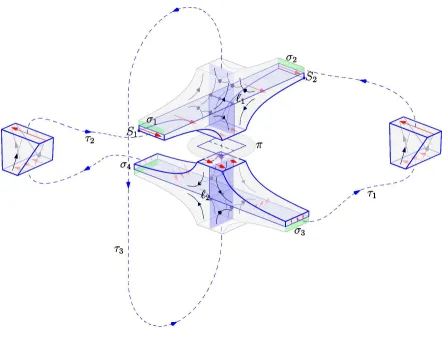
The following model for the fluid flow on a 3-dimensional manifold, displayed in Figure 1.1,

has been suggested by Dr. O. Kozlovski. Topologically, the manifold is equivalent to a solid

3-dimensional body whose boundary is a sphere with three handles. The vector field has two

lines of saddlesℓ1 andℓ2, which are orthogonal to each other and do not intersect. Light blue

two-dimensional surfaces consist of separatrices of the saddles. Blue dashed lines with arrows

represent solid tubesτ1,...,4 with cylindrical boundaries that connect two surfaces. Dark blue

arrows stand for the velocity field of the fluid flow, and red arrows is the stationary initial

induction field B0. We assume that the fluid flow is stationary outside of a neighbourhood

of the manifold and its velocity tends to zero rapidly near the boundary. Blue boundaries

mark “the dynamo manifold”, where the exponential growth of the initial induction field

takes place.

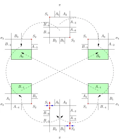
The induced mapping between the sections_{π, σ1,...,4}, is shown in Figure1.2. In particular,

we see that any point that leaves the dynamo manifold due to diffusion is being attracted

to the unstable manifolds of the saddles S1 and S2. In addition, we see two heteroclinic

connections clearly. To complete the construction one has to define gluing between the green

surfaces σ1,...,4 by tubes, and to make sure that unstable separatrices of two periodic saddle

pointsS1 andS2 eventually enter the tubeτ3. This will guarantee that all trajectories, that

leave the manifold due to diffusion, either return back shortly, and the frozen into the fluid1

magnetic field doesn’t change much, or go into a long tubeτ3, which causes large return time.

An alternative would be to make unstable separatrices to be attracted to periodic cycles of

1_{We say that a vector}_v_{field is frozen into a moving fluid if}_E₊_v_×_B_{= 0, which corresponds}_σ_≫_{1 in the}

Ohm’s law (1.4). In practice, it means that when a surface consisting of magnetic field lines is moved by

(18)

[image:18.595.106.548.89.427.2]

1.4 POINCAR´E MAP

Figure 1.1: Dynamo manifold with the fluid flow (blue) and magnetic induction field (red).

The labelsS1 and S2 mark periodic saddle points.

a huge period. This seems to be possible, although we are still working on the details.

We also would like to point out, that any small perturbation of the presented 3-dimensional

flow possess fast dynamo action as well. Therefore, once this example is verified, we will be

able to show that dynamo flows are generic.

1.4 Poincar´

e map

In order to study the flow, one can consider a global Poincar´e sectionπ, and the first return

mapF. The intersection between the plane π and the dynamo manifold has four connected

(19)

1.4 POINCAR´E MAP

“a square” which is shown in Figure 1.1. The restriction of the Poincar´e map onto the

square is representative for studying the flow action; and deserves a special consideration. In

particular, it is an unfolded1 Baker’s map and demonstrates chaotic properties. Since near

the intersection with the separatrices of the saddlesℓ2 the first return time is huge, a proper

2-dimensional model for the Poincar´e map would be a map with aZ-shaped hole, as shown

in Figure 1.3.

Outside of the square the first return map F has the following properties.

1. It is piecewise continuous and bijective.

2. It is area preserving.

3. The Euclidean norm of the differential is uniformly bounded_kdF_{k ≤}1 +µfor a small

µ >0.

4. The Hessian is small _kd2_F_{k ≤}_µ

2 for a small µ2 >0.

In addition, we shall impose an artificial condition in order to guarantee that the map outside

of the unit square doesn’t “bend” too much. This condition in principle should be replaced

by a statement similar to Yomdin’s Lemma on volume growth [35].

Consequently, as a first step we may try to show that the unfolded Baker’s map itself is a

fast dynamo in the presence of slow diffusion through the boundary. This is the main result

of the present work (Theorem9 p.162).

1_{In literature two different maps are being referred to as “Baker’s map”. By unfolded we mean the one that}

(20)

1.5 PRINCIPAL OBSTACLES AND GENERAL STRATEGY

1.5 Principal obstacles and general strategy

In the absence of diffusion (ε= 0) we may choose the initial magnetic fieldB0 to be collinear

with the stretching direction of the Baker’s map on the square and then transfer it out all

over the dynamo manifold using the fluid flow. The added diffusion makes the energy of the

vector field to dissipate through the boundary as a solution of the heat equation. Baker’s

maps were suggested as a model for kinematic fast dynamo long ago ([13], for example), and

a numerical evidence was found for the exponential growth of magnetic energy [12]. However,

there was no rigorous analytical argument in the presence of diffusion.

In order to be more specific, let us introduce a shorthand notation for the unit square

: =_{(x, y)_∈R2

| |x_|<1, _|y_|<1_}.

and consider the unfolded Baker’s map

P(x, y) =

                    

x−1

2 ,2y+ 1

, ifx_∈,₋1< y <0,

x+1

2 ,2y−1

, ifx_∈, 0< y <1,

F(x, y), if (x, y)_∈R2_\_;

(1.11)

where F:R2 _\ _→ _R2_\ _{is an area-preserving piecewise diffeomorphism with uniformly}

bounded Jacobian_k∂F_k<1 +µ(as the Euclidean norm of a linear operator) and such that

any point has not more thand_≪M preimages with respect to FM _{for some large} _M_{. Our}

goal is to show that there exists a vector fieldB0 such that

lim

ε→0nlim→∞

1

nln Z

R2

(exp(ε∆)P_∗)nB0

>0. (1.12)

It is sufficient to construct two cones C1 and C2 in the space of essentially bounded vector

fields with finite_L1 norm such that for someδ >0 and any sufficiently largem

(exp(ε∆)P_∗)m(C1)(C2(C1 and k(exp(ε∆)P∗)m |C1 k ≥(1 +δ)

(21)

The argument is based on the following ideas.

Noise instead of diffusion. The idea to replace the diffusion by noise added to the system

has been used by Klapper and Young in [19]. One can introduce a “small perturbation” of

the original map

Pt: =P+t

and associate a composition of small perturbations to any sequence ¯t_∈ℓ_∞(R2_{) by}

Pt¯m: =Ptm◦Ptm−1◦. . .◦Pt0.

Then by the Noise Lemma2.2.1withbt= 0, tm−1, . . . , t1:

(exp(ε∆)P_∗)mv(z) =

Z

R2(n−1)

wε(t1)wε(t2). . . wε(tm−1)(exp(ε∆)P_b_tm_∗v)(z)dt1dt2. . .dtm−1,

(1.13)

wherewε is the two-dimensional Gaussian kernel with isotropic varianceε, defined by (1.10).

It follows that it is enough to construct a pair of cones C1 and C2 such that for arbitrary

sequence of small vectors bt

exp(ε∆)P_b_tm

∗(C1)(C2 (C1 and kexp(ε∆)P

m

b

t∗ |C1 k ≥(1 +δ)

m

The choice of the norm. By definition, a cone is a convex subset which is invariant with

respect to multiplication by a non-negative real number. The cones we will be dealing with

have a general form

Cone (vk, αk) : ={dvk+w| kwk ≤d2−αkkvkk, d∈R+}.

We say that the cone Cone (v1, α1) is smaller than the cone Cone (v2, α2), if α1 > α2 > 0.

(22)

In order to construct a pair of cones, it helps to choose the norm in a proper way. The

diffusion represented by convolution with the Gaussian kernel means that the energy of a

vector field that changes direction rapidly cannot grow very fast due to cancellations [14].

It is not unreasonable to suggest therefore that piecewise constant vector fields will grow

rapidly. Following this idea, we introduce a class _G(m, δ) of partitions of the real plane with

the following properties.

1. The unit squarecontains at most 4m _{and at least 4}m−1 _{elements of the partition; the}

interior of an element of the partition does not intersect the boundary of the square.

2. Any element of the partition contains a square with side length _m12m and is contained

in a square with side length 2m+1.

3. Any square with a side δ may be covered by at most Nδ = 22m+1δ2 elements of the

partition.

To any partition Ω of the class _G(m, δ) we associate a weighted _L1 norm on the space of

vector fields by (cf. Subsection4.2.2):

kv_kΩ,L1

def

= X

ij

2−m

|πy(Ωij)|

Z

Ωij |v_|,

whereπy represents orthogonal projection onto the expanding direction of the Baker’s map.

The supremum norm of a vector field v we denote by _kv_k_∞def= sup_|v_|. Finally, on the space of essentially bounded vector fields with finite_L1norm, we introduce a new norm, combining

the two

kv_kdef= max_kv_kΩ,L1,2−

m/4_sup |v_|.

Canonical partitions. We would like to approximate the operator Pm

b

t∗ by a linear operator

(23)

matrix. In order to do that we construct a pair of so calledcanonical partitions Ω1 _{and Ω}2 _of

the class_G(m, δ), associated to a sequence of perturbationsbt(Subsection4.2.3) and introduce

two subspacesX_Ω1 andX_Ω2 of piecewise constant vector fields associated to partitions Ω1 and

Ω2_{, respectively. On every subspace of piecewise constant vector fields we choose a normalised}

basis

n

χs_Ω_ij def= 1

|πx(Ωij)|

(1

0)χΩij; χ

u

Ωij def

= 1

|πx(Ωij)|

(0 1)χΩij

o

i,j∈Z, (1.14) where πx represents the orthogonal projection onto the contracting direction of the Baker’s

map. The construction of canonical partitions rely on the study of small perturbations of

the doubling map. It is easy to observe that the Baker’s map and the doubling map are

closely related, and the former is just an extension of the latter. The canonical partition for

the sequencebtis set to be a direct product of two canonical partitions associated to suitably

chosen perturbations of the doubling map.

The first approximation. Once two partitions are chosen, we define a linear operator

At:XΩ1 →X_Ω2 by its matrix elements so that

Z Ω2

kl P_b_tm

∗v=

Z Ω2

kl

Atv for all Ω2kl∈Ω2 and anyv ∈XΩ1.

The choice of partitions allows us to establish the following facts about the matrix of the

operator_At in canonical bases (1.14).

1. There exists a small number 0 < γ1 < 0.01 such that sup_|akl_ij_| < 2γ1m_.

(Proposi-tion 4.3.2).

2. There exists an 15₁₆ < α < 1 such that for all _|t_{| ≤} 2−mα _{we have a decomposition}

At=Bt⊕ Ct. The matrix elements of the operator Bt satisfy (Proposition 4.3.1)

(24)

and the matrix of the operator_Ctis small

X

ckl_ij_≤100m(1 +µ)2m2−mα,

whereµ comes from the upper bound on the Jacobian ofF_|_R2_\.

Using the inequalities above, we deduce that for all sufficiently small _|¯t_{| ≤} 2−mα _{we have}

(Lemma 4.3.19)

kAt− A0k ≤2(2

3

4+γ1−α)m;

where _A0 corresponds to the zero sequence t = 0. Afterwards, we establish the following

facts

1. There exist two conesC1 ⊂XΩ1 and C₂ ⊂X_Ω2 such thatA_t(C₁)⊂C₂ andC₂ is much

smaller than C1 (Theorem8 p.141).

2. The operator _Atis a good approximation to Pbt∗ (Corollary 2 of Proposition4.3.3):

kexp(δ∆)(P_b_tm

∗ − At)νkΩ2 ≤2

2+(2+α)m_{sup diam(Ω}2

kl)kνkΩ1, where δ= 2−mα. (1.15)

The second approximation. The goal is to get rid of dependence of partitions Ω1 _{and Ω}2

on ¯tand to show that for any partition Ω3 of the class_G(m, δ) there exists a linear operator

D:X_→X_Ω3 such that for any δ= 2−mα and any |t| ≤δ the following properties hold true:

1. There exists a cone C3 _∈X_Ω3, smaller than the cone C1, such that (Proposition 4.4.4):

Dexp(δ∆)_At(C1)⊂C3.

2. The norm of the operator Dexp(δ∆)_At grows exponentially with m: for any v ∈XΩ1

we have (Lemma4.4.4):

kDexp(δ∆)_AtvkΩ3 ≥ 22m−2 3

(25)

1.6 OUTLINE

3. The operatorsDexp(δ∆)_Atand exp(δ∆)Atare close. There exists a smallγ2>0 such

that for anyv_∈X_Ω1 we have (Lemma 4.4.1):

k(Dexp(δ∆)_At−exp(δ∆)At)vkΩ3 ≤2(2−γ2)mkvk_Ω1. (1.16)

Combining the first (1.15) and the second (1.16) approximations, we get an invariant

cone for the operator exp(δ∆)P_b_t2m

∗ and derive from it an invariant cone for the operator

(exp(δ∆)P_∗)2m_.

It may seem at first sight that the examples chosen are too simple since they are linear.

However, it appears that they are sufficiently complicated to analyse and the same approach

is applicable to non-trivial perturbations, since most estimates are based on distortion

prop-erties and the distortion is easy to control for perturbations of hyperbolic maps.

1.6 Outline

The work presented has three chapters. In chapter2 “A proof of the fast dynamo theorem”

we give sufficient conditions (Invariant Cone Hypothesis1) for a piecewiseC2 transformation

ofRn_{to be a fast dynamo. In the following Chapters}₃_and₄_{we construct measure-preserving}

piecewise-C2 transformations ℓ: R _→ R and T: R2 _→ _R2_{, respectively, that satisfy the}

Hypothesis. As mentioned above, the arguments in the two-dimensional case rely on some

parts of the analysis of the one-dimensional system.

We begin the Chapter 2 with a few general constructions; we give a definition to small

random perturbations (Subsection 2.1.1), introduce a norm in the space of vector fields, and

fix the type of cones we are interested in. Then we explain how to reduce the system with

diffusion to a system generated by a small random perturbation of a certain map. Finally,

(26)

1.6 OUTLINE

Hypothesis.

The Chapter 3 we start with a few definitions, that introduce the central elements of

the construction. In particular, we define a class of partitions _G(m) of the real line with

a certain “uniform” property (Definition 4, p. 34); and a norm in the space of essentially

bounded integrable functions we will be using throughout (Definition3, p.26). In addition,

we introduce a transfer operator, that we will use to define an induced action of a piecewise

diffeomorphism on functions (Definition 5 p.35).

In Section 3.2.1 we consider a so-called toy dynamo operator between two linear spaces

A: X1 → X2 in the most abstract way, i.e. in terms of its matrix coefficients. We show

that for any toy dynamo operator there exist two cones C1 ⊂ X1 and C2 ⊂ X2 such that

A(C1)(C2; and C2 is much smaller than C1. This is the content of Theorem 3p. 45.

In Section 3.2 we show that a toy dynamo operator approximates a transfer operator,

induced by a large iteration mof a small random perturbation of the so-called dynamo map

(Subsection3.1). The dynamo map is an expanding map on the unit interval complemented

by reflection outside. More precisely, given 1< s2 <2< s1 <3, we define (3.3)

ℓ(x) =

                    

s1x+s1−1, if −1< x < _s2₁ −1;

s2x+ 1₋s2, if _s2₁ < x <1;

−x, otherwise;

and associate a small random perturbation to any sequence ξ _∈ ℓ_∞(R). Essentially, the toy dynamo operator is given by the transition matrix between two partitions of the class

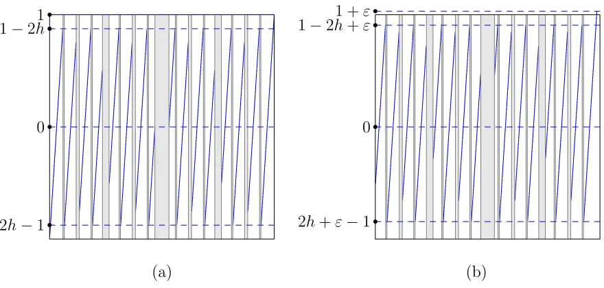
G(m) associated a small perturbation ℓm_ξ of the map ℓ. Namely, we see that aij = 1 if

ℓm_ξ (Ω1_i)_∩Ω_j2 = Ω2_j and ℓm_ξ _|_Ω1

i is increasing. Figure 1.4 shows a few iterations of the map

without perturbation (ξ_≡0) and with the largest possible perturbation (ξ _≡δ). We see that

(27)

1.6 OUTLINE

In Subsection 3.2.2we introduce a canonical partition Ωξ _{of the class} _G₍_m_{), associated to}

a small perturbation ξ. The partition has the following property. For any interval I with

ℓk_ξ(I)_⊂[₋1,1] for all 0_≤k < mthere exists an element of the partition Ωξ_i such thatI _⊆Ωξ_i.

In addition, the partition is “uniform”: any interval of the lengthδ contains not more than

Nδ elements of the partition.

In Subsection 3.2.3 we show that the operator ℓm_ξ_∗ may be very well approximated (The-orem 4 on p. 62) by a toy dynamo operator _T defined on the space of piecewise constant

functions associated to Ωξ. For any essentially bounded and absolutely integrable functionf,

k(ℓm_ξ_∗_{− T}) exp(δ∆)f_k2 ≤ _s3

1δ

21/2_s 2

m

·m_kf_k1.

Here we can choose parameters s1,s2 of the map ℓ, and a constantα such that the

approxi-mation is good enough: namely_{kT k}= 2m and

s3₁

21/2+α_s2 <2.

In Section 3.3 we construct an invariant cone for the operator exp(δ∆)ℓm_ξ_∗exp(δ∆) in the space of essentially bounded absolutely integrable functions. In order to do that, we

show that the image of the Weierstrass transform with Gaussian kernel with isotropic

vari-anceδ = 2−mα _≫sup_|Ω1_j_|may be well approximated by step functions on a partition Ω1 of the class _G(m). Namely, for any partition Ω2 _{of the class}_G₍_m_{) we have (Lemma}_3.3.2_):

kDΩ1W_δf−W_δfk₁≤

max(sup_|Ω1

j|,sup|Ω2j|)

δ kfk2≤

1

sm₂ δkfk2.

Based on this simple idea, we construct an invariant cone in the space of essentially bounded

integrable functions “around” the cone in the space of piecewise constant functions.

In chapter 4 we construct a transformation T: R2 _→ _R2 _{that satisfies Invariant Cone}

(28)

1.6 OUTLINE

on the square and complement it by a non-expanding area preserving map outside. The

argument runs in a similar way to the one-dimensional case; and according to the general

strategy described above in Subsection1.5.

In the beginning we fix notation related to mappings ofR2 _{and vector fields. In particular,}

we define (4.3) the Gaussian kernel Wδ and the Weierstrass transform operator on vector

fields.

In Section 4.2, we define the dynamical system we will be working with. It is easy to see

that the energy of the vector fields that change direction rapidly does not grow exponentially

fast. We are going, as before, to replace diffusion by small random perturbations, and we

have almost no control on the map outside the square. Therefore we need to introduce a

delay in return time artificially. One of possible solutions is to use atower construction.

In Subsection4.2.1we define the phase spaceXto be atower ofM floors, which is a union

of the real planeR2 _and _M₋_{1 copies of it with the central square cut off:}

X def= _{0_{} ×}R2

∪ {1, . . . , M ₋1_{} ×}(R2 \),

where = [₋1,1]2. We also define a map F:X _→ X, to be, generally speaking, Baker’s

map on the squareand some area-preserving map transferring points outside of the square

to a different floor.

F(z, n)def=

          

(F0(z),0), ifn= 0 and z∈;

(Fn+1(z),(n+ 1)mod (M−1)), otherwise.

(4.5)

(See p. 97 for definition of the maps Fn, n = 1, . . . , M −1.) We also introduce small

per-turbationsFξ of the map F. Afterwards, we define the mapP:R2 →R2 we will be dealing

with as a large iteration of the map Fξ.

In Subsection 4.2.2, we introduce (4.11) a norm on the space of vector fields we will be

(29)

1.6 OUTLINE

case, but we “weight” _L1 norm only in expanding direction. A linear operator we define to

be an action induced by P_ξ2 in ordinary way (4.10).

In Subsection 4.2.3 we exploit similarities between Baker’s map, its inverse, and the

dou-bling map, and construct a canonical partition for the Baker’s map as a direct product of

two partitions for suitably chosen small random perturbations of the doubling map.

In Section 4.3 we introduce a subspace X_Ω1 of piecewise constant vector fields associated

to the canonical partition Ω1_{. We define the basis on} _X

Ω1 to beV_Ωs1∪V_Ωu1, where

V_Ωs1

def

= n 1

|πx(Ω1_ij)|

(1 0)χΩ1

ij o

i∈Z,j∈Z and V

u

Ω1

def

= n 1

|πx(Ω1_ij)|

(0 1)χΩ1

ij o

i∈Z,j∈Z. The vectors that have only χΩs

ij components, are parallel to the contracting direction of the

Baker’s map and vectors that have only χΩu

ij components, are parallel to the expanding

di-rection of the Baker’s map. Using the operatorPξ∗, we define an associated linear operatorA

betweenX_Ω1 and a suitable subspace of piecewise constant vector fieldsX_Ω2 and such that

Z Ω2

kl

P_ξ2_∗ν =

Z Ω2

kl

Aν (4.16)

via its matrix elements. It is natural to write the operator _A as a direct sum of four linear

operators_A=SS_⊕SU _⊕U S_⊕U U, where

SS:_hV_Ωs1i → hV_Ωs2i; SU:hV_Ωs1i → hV_Ωu2i; U S:hV_Ωu1i → hV_Ωs2i; U U:hV_Ωu1i → hV_Ωu2i.

The growth of the energy is guaranteed by the operator U U, and we will study it separately

in the next section. We conclude this section with construction of a pair of cones C1 _⊂X_Ω1

and C2⊂XΩ2, such that A(C₁)(C₂ and the cone C₁ is much smaller than C₂.

In Subsection4.3.1we establish that the matrix of the operatorU U demonstrates properties

similar to the ones of “toy dynamo operator” we studied in the Chapter3. Namely, its central

part, corresponding to the elements from the unit square, has a plenty of 1’s, and the absolute

(30)

1.6 OUTLINE

In Subsection4.3.2we justify the choice of the operator _A, and show that operators WδA

andWδPξ2 are close on the subspace of piecewise constant vector fieldsXΩ1. The estimations

are based on the fact thatδ is chosen so that

max(sup_|πx(Ω2ij)|,sup|πy(Ω2ij)|)≪δ

and the construction of canonical partitions.

In Subsection 4.3.3 we construct a pair of cones for the operator _A, the larger cone

C1 ⊂ XΩ1 and a much smaller cone A(C₁) ⊂ C₂ ⊂ X_Ω2. We use the decomposition

A = SS _⊕SU _⊕U S _⊕U U, and exploit simplicity of the matrix U U along with upper

bounds on other operators.

The Subsection4.4.1repeats the Section3.3of the one-dimensional Chapter3with obvious

modifications adjusting the arguments to dimension two. In particular, the length of the

intervals of the partitions in the upper bounds is replaced by the diameter of the elements.

In Subsection 4.4.2we construct of an invariant cone for the operatorW δ

2mP 2

ξ∗W δ

(31)

1.6 OUTLINE

A4

A₋₁

B₁

B₋4 B₋5

A₃

A₋₂

B0 B₋3

B₋₆

A₅ A₂

A₋3 A₋6

B5 B2 B₋₂

B₃

A₋5

A0

A₁

B₋₁

B4

A₋4

B₋₃ B₋₆

A₅ A₂

A₋3 A₋₆

B5 B2

σ₁ S1

σ4 S1

π

S1

S₂

σ3 S2

σ₂

S2

π S₁

[image:31.595.134.523.140.592.2]

S₂

Figure 1.2: The mapping between the sections π, σ1,...,4, induced by the fluid flow;

Ak = Φ′(Ak−1), Bk = Φ′′(Bk−1). The points S1 and S2 are periodic saddles;

(32)

1.6 OUTLINE

x−1

2 ,2y+ 1

x+1

2 ,2y−1

[image:32.595.111.548.120.274.2]

(a) (b) (c)

Figure 1.3: (a) Unfolded Baker’s map, that appears as the first return map to the section π;

(b) Doubling map with a hole; and (c) a small perturbation of the doubling map

with a hole.

0 1

2h₋1 1₋2h

(a)

0 1 +ε

2h+ε₋1 1₋2h+ε

(b)

Figure 1.4: First four iterations of a small perturbation of the doubling map with a hole of

the widthh: (a) the case of the zero sequence; and (b) the case of the constant

[image:32.595.110.550.418.628.2]

(33)

2 A proof of the fast dynamo theorem

In this Chapter we give a proof for the fast dynamo theorem for maps satisfying certain

hypothesis. Later, in the Chapter 3 we construct a one-dimensional map satisfying this

hypothesis and in the Chapter 4 we prove that its two-dimensional extension also satisfies

these conditions. The two-dimensional map may be realised as a Poincar´e map of a smooth

stationary vector field in R3_.

2.1 Basic constructions

In this Section we introduce objects central for our investigations: small random perturbations

of a dynamical system and a norm in the space of vector fields. We also specify the type of

cones in the space vector fields we are interested in.

2.1.1 Small random perturbations

We construct a random dynamical system using skew-products. Let X be a real manifold

and letf:X_→X be a transformation. We consider its extension

b

(34)

2.1 BASIC CONSTRUCTIONS

Let Σ_⊂ℓ_∞(Rn_{) be a shift-invariant subset of two-sided bounded sequences of vectors in}_Rn_.

We introduce a skew product over the Bernoulli shift

σ_×fb: Σ_×X _→Σ_×X (σ_×fb)(ξ, z)def= (σ(ξ),fb(z, ξ(1))). (2.2)

The induced transformation on fibers we denote by

fξ:X →X, fξ(z)def= fb(z, ξ(1)). (2.3)

Its iterations are given by

f_ξk(z)def= fb(f_ξk−1(z), ξ(k)). (2.4)

Remark 1. The following identities follow from the definition of the mapfξ.

f_ξk=f_ξ₍_k₎_◦f_ξ₍_k₋₁₎_◦. . ._◦f_ξ₍₁₎; (2.5)

f_ξ−k= (f_ξk)−1=f_ξ−₍₁₎1 _◦f_ξ−₍₂₎1 _◦. . ._◦f_ξ−₍_k1₎; (2.6)

f_ξn−k=f_ξn_◦f_ξ−k=f_ξ−k_◦f_ξn=

          

f_σnn−₍k_ξ₎, ifn < k;

f_σnk−₍k_ξ₎, ifn > k.

(2.7)

Definition 2. We call the map fξ a random perturbation of the map f associated to the

sequence ξ_∈Σ.

2.1.2 Norm in the space of vector fields

Piecewise constant vector fields are proved to be very useful to us. We define a norm in the

space of essentially bounded and absolutely integrable vector fields Φ, using partitions.

The norm we are about to introduce is related to the mapf. Since topological entropy is

an upper bound for the growth rate of the energy, the system has to be chaotic. We shall

(35)

2.1 BASIC CONSTRUCTIONS

We let πu to be projection along the unstable foliation onto the stable manifold. We denote

by λnu thenu-dimensional Lebeague measure on the unstable manifold.

Let us fix a large number m_≫1. Its role will be clarified in the next Subsection.

Definition 3. A norm in the space of essentially bounded and absolutely integrable functions,

associated to a partition Ω(m) = ∞S

j=1

Ωj of Rn is given by

kf_kΩ = max X

j∈Z

2−num λnu(πu(Ωj))

Z Ωj

|f(x)_|dx,2−αmsup_|f_|; (2.8)

where the choice of α depends onn.

The first term we refer to as the weighted _L1-norm and write

kf_kΩ,L1: =

X

j∈Z

Z Ωj

|f(x)_|dx,

it depends, of course, on the partition chosen.

We denote by ΦΩthe subspace of Φ, consisting of piecewise constant vector fields associated

to the partition Ω.

2.1.3 Cones in vector fields on Rn

We reserve a notation for a cone of the radiusr with the main axis v0 in the space ΦΩ:

Cone (v0, r,Ω)def=nη=dv0+ϕ_|ϕ_∈ΦΩ, Z

(f_∗mϕ)v0 = 0;_kϕ_kΩ ≤drkv0k o

. (2.9)

We extend the cone Cone (v0, r,Ω) to include general functions from the main space:

[

Cone (v0, r, ε,Ω)def= n

f =η+g,_|η _∈Cone (v0, r,Ω),kgkΩ≤εkηkΩ o

. (2.10)

We say that the cone Cone[ v0, r1, ε1,Ω1 is smaller than the cone Cone[ v0, r2, ε2,Ω2 and write Cone[ v0, r1, ε1,Ω1 ≪ Cone[ v0, r2, ε2,Ω2, if r1 > r2 and ε1 > ε2; we do not assume

(36)

2.2 PROOF OF THE MAIN RESULT

2.2 Fast dynamo theorem

In this Section we set the hypothesis and give a proof of the fast dynamo theorem1.

The first step the Noise Lemma2.2.1, which suggests to replace the operator (exp(δ∆)f_∗)n in our considerations with the operator exp(δ∆)fn

t∗ for some sequence t.

We begin with a simple observation that the exponent of the Laplacian operator1 inRn_,

is the convolution with the Gaussian kernel, in particular

exp(δ∆)v=wδ∗v, wherewδ(x) =

1

√

2πδ exp − x2

2δ2

.

The latter operator is also known as the Weiertstrass transform Wδ(v) def= (wδ ∗ v); this

notation we use throughout.

The following statement is generally known, but we give a proof for completeness.

Lemma 2.2.1 (Noise Lemma). For any mapf:Rn_→ _Rn _{and for any vector field} _v _in _Rn

we have

Wδ

2f∗(Wδf∗)

m−1_v₍_x_{) =}Z

Rn(m−1)

wδ(t1)wδ(t2). . . wδ(tm−1)(Wδ

2f

m

0t∗v)(x)dt1dt2. . .dtm−1,

(2.11)

where 0t= (0, t1, t2, . . . , tm−1)∈Rm.

Proof. Observe that f−1₍_x₋_t_{) =} _f−1

t (x), because ft(x) = f(x) +t. By straightforward

(37)

calculation,

Wδ

2f∗(Wδf∗)

m−1_v₍_x_{) =}_W δ

2f∗(Wδf∗)

m−2_W

δf∗v(x) =

=Wδ

2f∗(Wδf∗)

m−2Z

Rn

wδ(t)(f∗v)(x−t)dt=

=Wδ

2f∗(Wδf∗)

m−2Z

Rn

wδ(t1)(ft1∗v)(x)dt1 =. . .=

=Wδ

2

Z

Rn(m−1)

wδ(t1). . . wδ(tm−1)(f∗ft1∗. . . ftm−1∗v)(x)dt1. . .dtm−1=

=

Z

Rn(m−1)

wδ(t1). . . wδ(tm−1)(Wδ

2f

m

0t∗v)(x)dt1. . .dtm−1.

Corollary 1. For any mapf:Rn_→_Rn_{, any vector field}_v

0inRn, and for anyk=k0m≫m

Wδ

2f∗(Wδf∗)

k−1_W δ

2v0(x) = =

Z

Rk−k0

wδ(t1)wδ(t2). . . wδ(tk−k0)

Wδ

2f

m

0t∗Wδ2

k0

v0(x)dt1dt2. . .dtk−k0. (2.12)

We shall put the following conditions on the map f.

Hypothesis 1 (Invariant Cone). There exist an m_≫1, a partitionΩ(m), a vector field v0,

and four numbers r2(m) ≪ r1(m), ε2(m) ≪ ε1(m) ≪ 1 such that for any sequence ξ with

kξ_k_∞_≤δ

Wδ

2f

m

0t∗Wδ2: [

Cone (v0, r1, ε1,Ω)→Cone ([ v0, r2, ε2,Ω)⊂Cone ([ v0, r1, ε1,Ω) (2.13)

Moreover, there exists 0< γ <0.01 such that for any field v_∈Cone ([ v0, r1, ε1,Ω)

2m−2_kv_kΩ ≤ kWδ

2f

m

0t∗Wδ2vkΩ ≤2

(1+γ)m

kv_kΩ. (2.14)

We construct a map f:R _→ R satisfying this hypothesis in the Chapter 3 and a map

f:R2 _→_R2 _{satisfying this condition in the Chapter} ₄_.

We choose δ = 2−mα_{, a partition Ω = Ω(}_m_{) =} S_Ω

j, the vector field v0 ≥0, and fix four

(38)

Lemma 2.2.2. In the notations introduced above, for any v_∈Cone ([ v0, r1, ε1,Ω)

Z

[−δ,δ]m−1 wδ

m(t1). . . w δ

m(tm−1)(W δ

2mf

m t∗W δ

2mv)dt1. . .dtm−1 ∈

[

Cone v0, e2r2, e2ε2,Ω.

(2.15)

Proof. By the Hypothesis assumption, we know that for any _|t_{| ∈} [₋δ, δ]m and any vector

fieldv _∈Cone ([ v0, r1, ε1,Ω)

W δ

2mf

m t∗W δ

2mv =dv0+ψt+gt∈

[

Cone (v0, r2, ε2,Ω),

whereψt∈ΦΩ,kψtkΩ ≤dr2kv0kΩ andkgtkΩ≤dε2kv0kΩ. Observe that Ω is independent on

t. Therefore,

Z

[−δ,δ]m−1 wδ

m(t1). . . w δ

m(tm−1)v0dt1. . .dtm−1 =

=v0 Z δ

−δ

wδ m(t)dt

m−1

=v0

1₋ 2

m m−1

≥e−2v0, (2.16)

form large enough. Sinceψt∈ΦΩ for any t∈[−δ, δ]m,

Z

[−δ,δ]m wδ

m(t1). . . wmδ (tm−1)ψtdt1. . .dtm−1 ∈ΦΩ,

and we calculate Ω-norm.

Z

[−δ,δ]m−1

wδ

m(t1). . . wmδ(tm−1)ψtdt1. . .dtm−1 _Ω≤

≤X

j∈Z

Z

[−δ,δ]m−1 wδ

m(t1). . . w δ

m(tm−1) Z

Ωj

|ψt(x)|dx

dt1. . .dtm−1≤

≤sup

t k

ψtkΩ≤dr2kv0kΩ.

Similarly,

Z

[−δ,δ]m−1 wδ

m(t1). . . w δ

m(tm−1)gtdt1. . .dtm−1

(39)

Observe that

Z 1

−1 Z

[−δ,δ]m−1

wδ

m(t1). . . w δ

m(tm−1)ψt(x)dt1. . .dtm−1dx=

=

Z

[−δ,δ]m−1 wδ

m(t1). . . w δ

m(tm−1)dt1. . .dtm−1· Z 1

−1

ψt(x)dx= 0.

Summing up, for any v_∈Cone ([ v0, ε1, r1,Ω)

Z

[−δ,δ]m−1 wδ

m(t1). . . w δ

m(tm−1)W δ

2mf

m t∗W δ

2mvdt1. . .dtm−1 ∈

[

Cone v0, e2r2, e2ε2,Ω.

Lemma 2.2.3. In the notations introduced above, assume in addition that2γm_e−m_≪_ε

2(m).

Then

W δ

2mf∗(Wδf∗)

m−1_W δ

2m:

[

Cone (v0, r1, ε1,Ω)→Cone[ v0, e2r2, e2ε2,Ω( [Cone (v0, r1, ε1,Ω) ;

Moreover, there exists 0< γ <0.01 such that for any field v_∈Cone ([ v0, r1, ε1,Ω)

2m−5_kv_kΩ≤ kW δ

2mf∗(Wδf∗)

m−1_W δ

2mvkΩ ≤2

(1+γ)m_k_v_k

Ω

Proof. By Lemma2.2.1 for any v_∈Cone (v0, r1,Ω)

W δ

2mf∗(W δ mf∗)

m−1_W δ

2mv=

=

Z

Rm−1 wδ

m(t1). . . w δ

m(tm−1)(W δ

2mf

m t∗W δ

2mv)dt1dt2. . .dtm−1=

=Z

Rm−1_\_[₋_δ,δ_]m−1 +

Z

[−δ,δ]m−1

m_Y−1

j=1 wδ

m(tj)(W δ

2mf

m t∗W δ

2mv)dt. (2.17)

By Lemma2.2.2we know that for anyv_∈Cone ([ v0, r1, ε1,Ω)

Z

[−δ,δ]m−1

m_Y−1

j=1 wδ

m(tj)(W δ

2mf

m t∗W δ

2mv)dt∈

[

(40)

We estimate the first term

Z

Rm−1_\_[₋_δ,δ_]m−1

m_Y−1

j=1 wδ

m(tj)(W δ

2mf

m t∗W δ

2mv)dt

Ω ≤

≤X

j∈Z

Z

Rm−1_\[−δ,δ]m−1

m_Y−1

j=1 wδ

m(tj) Z

Ωj W δ

2mf

m t∗W δ

2mv(x)

dxdt_≤

≤sup

t k

W δ

2mf

m t∗W δ

2mvkΩ Z

Rm−1_\[−δ,δ]m−1

m_Y−1

j=1 wδ

m(tj)dt.

We shall find an upper bound for the integral:

Z

Rm−1_\_[₋_δ,δ_]m−1

m_Y−1

j=1 wδ

m(tj)dt≤ ≤2mZ

+∞

δ

wδ m(t)dt

m

+ 2m Z +∞

δ

Z

[−δ,δ]m−1

wδ

m(t1). . . w δ

m(tm−1)dt1. . .dtm−1 ≤ ≤2me−m2+ 2me−m.

We may also recall that there exists 0< γ < 0.01 such that for any v _∈Cone ([ v0, r1, ε1,Ω),

we have sup_t_kW δ

2mf

m t∗W δ

2mvkΩ ≤2

(1+γ)m_k_v_k

Ω. Therefore

sup

t k

W δ

2mf

m t∗W δ

2mvkΩ Z

Rm−1_\[−δ,δ]m−1

m_Y−1

j=1 wδ

m(tj)dt≤2

(1+γ)m_·₂_me−m_k_f_k

Ω.

We need to verify 2(1+γ)m_·₂_me−m _≪₂m−5_ε

2, which is equivalent to 2γm+6e−m≪ε2.

For the second inequality we recall the second condition of the Hypothesis

∀v_∈Cone ([ v0, r1, ε1,Ω) :kW δ

2mf

m ξ∗W δ

2mvkΩ≥2

m−2_k_v_k Ω. Then Z

[−δ,δ]m−1

m_Y−1

j=1 wδ

m(tj)(W2δmf

m t∗W δ

2mv)dt _Ω≥

≥ inf

t∈[−δ,δ]mkW2δmf

m t∗W δ

2mvkΩ· Z

[−δ,δ]m−1

m_Y−1

j=1 wδ

m(tj)≥2

m−2_e−2_k_v_k

Ω. (2.18)

Taking into account

Z

Rm−1_\_[₋_δ,δ_]m−1

m_Y−1

j=1 wδ

m(tj)(W2δmf

m t∗W δ

2mv)dt

Ω≤2

m_ε

(41)

we get the result.

Theorem 1 (Fast dynamo theorem). Let f:Rn _→ _Rn _{be a piecewise-C}2 _{transformation}

satisfying the Invariant Cone Hypothesis and an additional condition 2_eγm _≪ ε2. Then there exists an essentially bounded vector field v, with absolutely integrable components such

that

lim

δ→0nlim→∞

1

nln

(exp(δ∆)f_∗)nv

L1 >0,

Proof. It follows by straightforward calculation that WδWδ = W2δ for any number δ > 0.

The Theorem follows from Corollorary1 of Lemma2.2.1and Lemma2.2.3withv=W δ

2mv0.

(42)

3 Fast dynamo on the real line

This Chapter is dedicated to the construction of a transformation ℓ:R → R satisfying the

Invariant Cone Hypothesis1, p.28. In perspective, the operatorℓ_∗corresponds to the induced action on vector fields on the unstable manifold of the Poincar´e map of the provisional flow.

The unstable manifold is one dimensional and the settings are the following. Vector fields

on a one-dimensional real manifold may be identified with functions R_→R; and an induced

action on vector fields on R is given by a transfer operator (ℓ_∗v)(y) = P

x∈ℓ−1₍_y₎

dℓ(x)v(x),

whereℓ:R→R is a piecewise-differentiable function.

The main result is the following

Theorem 2 (Invariant cone). There exist a measure preserving piecewise-smooth

transfor-mationℓ:R_→R, a cone C in the space Φof essentially bounded absolutely integrable vector

fields on R, and a norm _{k · k} in Φ such that for an m _≫ 1 large enough and any sequence

kξ_k_∞_≤δ with δ= 2−mα for 15₁₆ < α <1 we have

W δ

2mℓ

m ξ∗W δ

2m:C→C; ∀f ∈C:kW δ

2mℓ

m ξ∗W δ

2mfk ≥

1 4kℓ

m

∗ k · kfk. (3.1)

3.1 Notation

(43)

3.1 NOTATION

The following letters are reserved for constants: α, β, γ, γ1, κ, s1, s2. The admissible

range of values will be specified later.

Given a subsetI _⊂Rn_{we denote by}_|_I_|_{its Lebesgue measure. We say that two sets}_I1 _and

I2 are δ-close and write |I1−I2|< δifI1 belongs to theδ-neighbourhood ofI2 orI2 belongs

to theδ-neighbourhood of I1. Otherwise, we write |I1−I2|> δ. The indicator function of a

set I we denote by χI.

Let δij be the Dirac delta function:

δij =

          

1, ifi=j

0, otherwise.

The supremum norm of a sequence of real numbersξ _∈ℓ_∞(R) we denote bykξ_k= sup

k∈N|

ξk|.

Whenever supremum or infimum are taken along the whole range of values, we omit the

range.

We write x_≪y when xis exponentially small compared toy, namely, there exist a small

number 0< ε <1 such thatx <2−εmy.

Let δ= 2−mα be a small real number with 15₁₆ < α <1.

Definition 4. We say that a collection of intervals Ω = _{Ωj}j∈Z makes a partition of the

class _G(m, δ, s1, s2), if SΩj =R, Ωi∩Ωj =∅ifi6=j, and the following conditions hold true.

1. The interval [₋1,1] contains at least 2m−1 _{and at most 2}m _{intervals of the partition,}

and _{±1_}are the end points of some intervals of the partition.

2. The length of intervals Ωj is bounded away from zero and from infinity

1

msm

1 ≤ |

Ωj| ≤2

₁ sm

1

+ 1

sm

2

(44)

3.1 NOTATION

3. Any intervalI _⊂R of the length_|I_|=δ contains not more than

Nδ = 2m+1δlogs12 = 2m(1−αlogs12)+1

intervals of the partition.

4. Any interval of the partition Ωj ⊂R\[−1−mδ,1 +mδ] has length|Ωj|= 2−m.

We write_G(m, δ, s1, s2) to indicate dependence onm,δ,s1, ands2; we will abuse notations

and omitm,δ,s1, ors2, when it leads to no confusion and the dependence is of no importance.

We number intervals of a partition Ω in the natural order, starting from Ω0 ∋0. We set

ΩNl to be the most left interval of Ω inside [−1,1], and ΩNr to be the most right interval of

Ω inside [₋1,1].

Here we deal with essentially bounded absolutely integrable functions on the real line. We

refer to the space Φdef= _L1(R)∩L∞(R) as the main space. “Any function” refers to a function

from the main space always.

Given a partition Ω = _{Ωj}j∈Z of the class G, we denote the associated space of step functions by ΦΩ and address the basis {χΩj}j∈Z as the canonical basis of ΦΩ.

Definition 5. We associate a weighted transfer operator f_∗, acting on the main space, to a mapf on the real line by1

(f_∗φ)(x) : = X

y∈f−1(x)

sgn df(y)φ(y). (3.2)

3.1.1 The dynamical system

Here we define the system we will be studying. We have specified the phase space to be the

space of essentially bounded and absolutely intgrable vector fields on R. Now we define a 1_{Transfer operator is a bounded linear operator. In this case, it is chosen to be one dimensional analogue}

of induced action on vector fields by area-preserving transformations. Transfer operators with negative

(45)

3.1 NOTATION

transformation and a norm. We also fix the type of cones we will be dealing with.

The transformation of Φ. Let s2 ≤2≤s1, be two real numbers such that logs_s1₂ =κ≪1.

and letδ = 2−mα be a small real number with 15₁₆ _≤α <1. Consider the map ℓ:R_→R

ℓ(x) =

                    

s1x+s1−1, if −1< x < _s2₁ −1;

s2x+ 1−s2, if _s2₁ −1< x <1;

−x, otherwise.

(3.3)

and define its extension bℓ:R2 _→_R_by _ℓ_b₍_{x, y}_{) =}_ℓ₍_x_{) +}_y_{. We associate a small perturbation} ℓξ to any sequence ξ∈ℓ∞(R) and kξk∞≤δ.

The mapℓoutside the unit interval is not important to us and we chose a simple map that

changes direction of the vector field, to make it non-trivial. The exact form is not relevant

here. We associate a transfer operator to a mapℓm

ξ according to (3.2). We will be studying

the actionℓm_ξ_∗: Φ_→Φ.

Norm in the space of vector fields. Piecewise constant vector fields have proved to be

very useful to us. We define a norm in the space Φ of essentially bounded and absolutely

integrable vector fields on R, using partitions.

Definition 6. A norm in the space ΦΩ of essentially bounded and absolutely integrable

functions, associated to a partition Ω = ∞S

j=1

Ωj of R, is given by

kf_kΩ = max X

j∈Z 2−m

|Ωj|

Z Ωj

|f(x)_|dx,2−m/2sup_|f_|. (3.4)

The first term we refer to as the weighted _L1-norm and write

kf_kΩ,L1: =

X

j∈Z 2−m

|Ωj|

Z Ωj

|f(x)_|dx,

(46)

3.2 DYNAMO OPERATOR

This definition agrees with general definition in Subsection 2.1.2withα = 1/2.

The subspace of Φ, consisting of piecewise constant vector fields associated to the

parti-tion Ω we denote by ΦΩ. Observe that for any step function φ = P

j∈Z

cjχΩj ∈ ΦΩ we have

that

kφ_kΩ = max

2−mX

j∈Z

|cj|,2−m/2sup|cj|

. (3.5)

Cones in vector fields on R. We reserve a notation for a cone of radius r with the main

axisχ_[₋₁_,_1] in the space ΦΩ of piecewise constant functions, associated to a partition Ω:

Cone (r,Ω)def=nη =dχ[−1,1]+ϕ|ϕ= X

j∈Z

cjχΩj;

Nr X

j=Nl

cj = 0; kϕkΩ≤dr o

. (3.6)

We extend the cone Cone (r,Ω) to include general functions from the main space:

[

Cone (r, ε,Ω)def= nf =η+g,_|η _∈Cone (r,Ω),_kg_kΩ ≤εkηkΩ o

. (3.7)

This definition agrees with general definition in Subsection 2.1.3.

3.2 Transfer operator as a dynamo operator

The plan is to choose suitable subspaces of Φ and approximate the operatorℓm_ξ_∗by an operator with a simple matrix. The latter we call ageneralised toy dynamo operator.

Afterwards, we prove that there exists a map ℓ:R→R such that for any small

perturba-tion ℓm_ξ with _kξ_k_∞ _≤ δ we can find a generalised toy dynamo operator _A: Φ_→ Φ and two partitions Ω1 and Ω2 ofRsuch that_A: ΦΩ1 →Φ_Ω2 and k(ℓm_ξ

∗− A)Wδk ≤2−γm(kℓmξ∗k+kAk)

for someγ >0.

3.2.1 Generalised toy dynamo operators

Here we give a definition and show that any generalised toy dynamo operator _A possess a

(47)

3.2 DYNAMO OPERATOR

Let_Abe a linear operator acting on the main space. Assume that there exists two partitions

Ω1, Ω2 of the class _G such that _A: Φ_Ω1 → Φ_Ω2. Here and below we denote by N_l1 and N_r1

the indices of the first and the last intervals of the partition Ω1 inside [₋1,1], respectively;

and letN2

l and Nr2 be the indices of the first and the last intervals of the partition Ω2 inside

[₋1,1], respectively. In other words, the sets Ω2_i _×Ω1_j with N_l2_≤i_≤N_r2, andN_l1 _≤j _≤N_r1

make a partition of the unit square.

We define several sets of indices in order to describe the properties of the operator _A

important to us. Let aij be coefficients of the matrix of A in the canonical bases of the

subspaces Φ_Ω1 and Φ_Ω2.

Accelerator:

Ar : =j_{∈ {}N_l1, . . . , N_r1_{} |}#_{i_{∈ {}N_l2, . . . , N_r2_{} |}aij = 1} ≥2m−Nδ . (3.8)

Inflow diffusion:

Din: =(i, j)∈ {Nl2, . . . , Nr2} × {Nl1, . . . , Nr1} |aij 6= 1 . (3.9)

Outflow diffusion:

Dout: ={Nl2−mNδ, . . . , Nr2+mNδ} × {Nl1−mNδ, . . . , Nr1+mNδ}−

− {N_l2, . . . , N_r2_{} × {}N_l1, . . . , N_r1_}. (3.10)

Indifferent subspace:

Sp : =Z2_{\ {}_N2

l −mNδ, . . . , Nr2+mNδ} × {Nl1−mNδ, . . . , Nr1+mNδ}. (3.11)

We are interested in linear operators _A such that the following conditions hold true for the

matrix coefficients in the canonical bases.

Kinematic fast dynamo problem

University of Warwick institutional repository: http://go.warwick.ac.uk/wrap

A Thesis Submitted for the Degree of PhD at the University of Warwick

http://go.warwick.ac.uk/wrap/66400

This thesis is made available online and is protected by original copyright.

Please scroll down to view the document itself.

Kinematic Fast Dynamo Problem

by

Polina Vytnova

A thesis submitted in partial fulfilment of the requirements

for the degree of

Doctor of Philosophy in Mathematics

Contents

List of Figures

Acknowledgements

Declarations

Abstract

1 Introduction

1.1 A problem of magnetohydrodynamics

1.2 Brief history

1.3 Provisional fluid flow

1.4 Poincar´

e map

1.5 Principal obstacles and general strategy

1.6 Outline

2 A proof of the fast dynamo theorem

2.1 Basic constructions

2.2 Fast dynamo theorem

3 Fast dynamo on the real line

3.1 Notation

3.2 Transfer operator as a dynamo operator