Active appearance pyramids for object parametrisation and fitting

warwick.ac.uk/lib-publications

Zhang, Qiang , Bhalerao, Abhir, Dickenson, Edward and Hutchinson, Charles. (2016) Active appearance pyramids for object parametrisation and fitting. Medical Image Analysis, 32 . pp. 101-114.

Permanent WRAP URL:

http://wrap.warwick.ac.uk/78863

Copyright and reuse:

The Warwick Research Archive Portal (WRAP) makes this work by researchers of the University of Warwick available open access under the following conditions. Copyright © and all moral rights to the version of the paper presented here belong to the individual author(s) and/or other copyright owners. To the extent reasonable and practicable the material made available in WRAP has been checked for eligibility before being made available.

Copies of full items can be used for personal research or study, educational, or not-for-profit purposes without prior permission or charge. Provided that the authors, title and full bibliographic details are credited, a hyperlink and/or URL is given for the original metadata page and the content is not changed in any way.

Publisher’s statement:

© 2016, Elsevier. Licensed under the Creative Commons Attribution-NonCommercial-NoDerivatives 4.0 International http://creativecommons.org/licenses/by-nc-nd/4.0/

A note on versions:

The version presented here may differ from the published version or, version of record, if you wish to cite this item you are advised to consult the publisher’s version. Please see the ‘permanent WRAP URL’ above for details on accessing the published version and note that access may require a subscription.

Active Appearance Pyramids for Object

Parametrisation and Fitting

Qiang Zhang1_{, Abhir Bhalerao}1_{, Edward Dickenson}2_{, and Charles Hutchinson}2

1_{Department of Computer Science, University of Warwick, Coventry, CV4 7AL, UK}

1_{University Hospitals Coventry and Warwickshire, Coventry, CV2 2DX, UK}

March 8, 2016

Abstract

Object class representation is one of the key problems in various medical image analysis tasks. We propose a part-based parametric appearance model we refer to as an Active Appearance Pyramid (AAP). The parts are delineated by multi-scale Local Feature Pyramids (LFPs) for superior spatial specificity and distinctiveness. An AAP models the variability within a population with local translations of multi-scale parts and linear appearance variations of the assembly of the parts. It can fit and represent new instances by adjusting the shape and appearance parameters. The fitting process uses a two-step iterative strategy: local landmark searching fol-lowed by shape regularisation. We present a simultaneous local feature searching and appearance fitting algorithm based on the weighted Lucas and Kanade method. A shape regulariser is derived to calculate the maximum likelihood shape with re-spect to the prior and multiple landmark candidates from multi-scale LFPs, with a compact closed-form solution. We apply the 2D AAP on the modelling of vari-ability in patients with lumbar spinal stenosis (LSS) and validate its performance on 200 studies consisting of routine axial and sagittal MRI scans. Intervertebral sagittal and parasagittal cross-sections are typically used for the diagnosis of LSS, we therefore build three AAPs on L3/4, L4/5 and L5/S1 axial cross-sections and three on parasagittal slices. Experiments show significant improvement in con-vergence range, robustness to local minima and segmentation precision compared with Constrained Local Models (CLMs), Active Shape Models (ASMs) and Ac-tive Appearance Models (AAMs), as well as superior performance in appearance reconstruction compared with AAMs. We also validate the performance on 3D CT volumes of hip joints from 38 studies. Compared to AAMs, AAPs achieve a higher segmentation and reconstruction precision. Moreover, AAPs have a significant im-provement in efficiency, consuming about half the memory and less than 10% of the training time and 15% of the testing time.

1

Introduction

Representation and segmentation of anatomical objects is of vital importance in the understanding of medical images. A standard approach which has proven robust and efficient, is to learn and leverage prior knowledge of the object garnered from statistics of its parametric form. To achieve this, the following steps are implemented: delineating the object class with a coherent parametric form; learning a prior model of the object class by formulating the statistics of the parameters; and fitting the parametric model to new, unseen instances while regularising the solution with the learned prior model.

The most commonly used strategy is to describe the objects with deformable appear-ances such as morphable models [1], statistical deformable models [2] and AAMs [3, 4]. The correspondence in the training data are established by annotating the landmarks at consistent features of interest from subjects. The prior knowledge is then usually learned through a linear model by applying eigen analysis, e.g. PCA. As a generative method, AAMs can not only achieve a robust segmentation, but also synthesise new instances and code the appearance with compact parameters for higher-level interpretation, such as for the diagnosis and grading of pathologies. AAMs are widely adopted and have proven successful, but in clinical applications face challenges such as their sensitivity to local minima during fitting, and computational costs when built on 3D data.

In addition to the holistic methods, part-based models have shown superior perfor-mance in computer vision tasks including object detection and tracking. Notable exam-ples are sub-model AAMs [5, 6], Deformable Part Models [7, 8, 9], Constrained Local Models [10, 11, 12] and mixture-of-trees models [13], in which an object is decomposed into locally rigid parts with a geometric model capturing spatial relationships among parts. Among these the models reported applied for clinical applications are sub-model AAMs and CLMs. For example in [11] the CLMs show superior performance over AAMs on brain and dental images. In [14] combined with random forests regression CLMs are re-ported to have the best performance in segmenting femur radiographs. The fitting process is implemented by local feature searching followed by a regularisation imposed through a prior model of the global shape. CLMs decompose the complex appearance into parts with simpler structures therefore suffer less from the high dimension low sample space (HDLSS) problem when compared to AAMs. Moreover they are able to utilise advanced feature detection algorithms such as boosted regression [15], random forests [14], regu-larised mean-sift [16], and shape optimisation methods such as pictorial structures [17]

and non-parametric model [18]. Due to the small local support of the feature patches

however, the local feature detectors in CLMs are plagued by the problem of ambiguity, which results in errors in landmark location as the detection becomes trapped in local minima [12]. In addition, the existing part-based models coarsely delineate the objects focussing on capturing the key features which is sufficient in computer vision tasks, but in clinical applications a more delicate appearance model is needed to preserve the structural details and parametrise the entire anatomical appearance.

appearance as well if not better than AAMs, and have superior performance in compu-tational efficiency and precision. Our work differ from the previous part-based models in that instead of fitting the shape, we focus on a parametric representation which can model and visualise the whole appearance variations within an object class, and fit the model to new instance to obtain the parametric representation of both the shape and appearance. The main contributions integrated in the proposed method are threefold: (1) A multi-scale Local Feature Pyramid (LFP) as the part delineation which offers a comprehensive description of the local feature and shows resistance to local minima; (2) An efficient AAP fitting algorithm derived from the weighted Lucas and Kanade (LK) methods [19]; (3) A shape regulariser integrating multiple landmark candidates from the LFPs, with a closed-form solution of the maximum likelihood (ML) shape.

In this paper, we detail how AAPs are constructed, trained and fitted and demonstrate that the appearance of an object can be delineated with multi-scale parts and that an associated deformation can be approximated by a set of locally rigid transformations of the parts. We set out the context of the problem in section 2 and detail the AAP in section 3. In section 4 we derive an efficient fitting algorithm based on the weighted LK method and a regulariser utilising multi-scale landmark candidates. In section 5 we apply 2D AAPs for modelling and fitting of lumbar vertebrae in axial and parasagittal MRI slices, which exhibit varied LSS. We demonstrate their performance against AAMs and CLMs by measuring the convergence range, segmentation accuracy and reconstruction precision. We also present experiments of 3D AAPs validated on CT data of the pelvis focussing on the hip joint. We compare the storage, computational saving as well as the segmentation and reconstruction quality against AAMs. We conclude with a discussion

of the relative merits of AAPs and give proposals for further improvement. 1

2

Background

The range of object representation and active fitting methods proposed in the literature strive to improve performance and precision. The methods have thus been adapted in various ways: to allow the prior models to compactly capture variation yet be able fit to unseen instances containing pathology; and prevent the fitting becoming trapped in local minima whilst maintaining a simplicity in object parametrisation and efficiency in fitting. We consider the challenge of local minima during fitting and how the choice of delineation (parametrisation) of objects can resolve this problem, but also result in a more flexible parts model which is efficient.

2.1

Local minima

Local minima are a problem facing all shape and appearance based methods. They not only reduce the convergence range, which affects the initialisation, but also introduce large errors to the fitting results. In both holistic and part-based methods, a coarse-to-fine strategy is often employed, which naturally increases the ‘capture range’ of the initialisation. However, even if at the finest level the model is close to the desired solution, the occurrence of local minima is still likely to divert the model from it [20].

Part-based models such as CLMs are plagued by the local minima problem due to their small local support and the large appearance variation. The most effective strategy

1_{Videos as well as other supplementary materials are available online at}

is to manipulate the scale. For instance, an efficient constrained mean shift method is proposed by [16, 12], in which a varying kernel density estimate (KDE) is applied to perform coarse-to-fine fitting. The method starts with a smooth unimodal Gaussian model, and refines the fidelity by reducing the smoothness and increasing the number of modes. [21] searches for the local patches with coarse-to-fine resolution and use the results as an initialisation for the AAM fitting. [22] use a hierarchy of shape models to extend the CLM where the relationships between landmarks at each level is modelled by a MRF: the local models ‘select’ the best candidate points and the global model acts as a regulariser. They demonstrate an improvement in performance over CLMs. Despite the optimisation in feature searching algorithms, the choice of the feature scale (size of the image patches) itself is a trade-off between the location specificity and textural properties. Also the features at different landmarks themselves can have salient edges at varying scales (see for example Fig. 2(b)), therefore an unitary scale for the descriptors across all landmarks will not capture faithfully all the salient features. We confirm that a LFP combining multi-scale local features at each landmark gives a more comprehensive description, and the shape fitting with multiple landmark estimations shows an ability to resist local minima.

2.2

Object class representation

In medical images, structural degeneration is often seen with the local appearance changes. For example in MRIs of patients with LSS, vertebral degeneration is often seen as an abnormal shape along with local intensity changes which could indicate facet joint thick-ening (Fig. 5(b)) and/or disc herniation (Fig. 5(c)) and occasionally inflammation or fractures. In this instance, because the intensity and structural variations are related and coupled, a combined parametric delineation of shape and appearance could therefore offer a more robust segmentation. Representative methods using combined model are AAMs and CLMs.

AAMs have proven successful, but face challenges in the context of medical image analysis because: (i) AAMs model the inner region of the shape mesh, but for organs with convex shapes, a large proportion of textures of the inner region offers limited information while consuming a majority of the computational resources. Instead, there can be richer information lying around the landmarks, at the periphery of an organ boundaries. Modelling the neighbourhood background can remedy this problem [23] but with an additional computational burden. (ii) The memory usage and computational cost increases significantly when modelling volumetric data. The efficiency is reduced by the image warping process, which is both expensive and complex to implement. Although there have been attempts to improve the tractability of 3D AAMs [24, 25], they have to either endure a large memory usage and slower speed, or sacrifice the precision by subsampling the data.

part-based appearance model which can enhance the robustness and precision but also parametrise the whole appearance for subsequent classification tasks such as diagnosis and grading.

Our approach is to start with a part-based model, by parametrising objects as an assembly of object parts, but with the parts being multi-scale local appearance captured by a LFP. This multi-scale approach overcomes problems of local minima when searching for landmark locations, and the pyramid allows the appearance model to fully cover the object interiors and capture the landmark context, allowing the resulting AAP to have generative capabilities. The part-based form also gives us flexibility in our choice of fitting strategy.

3

Active appearance pyramid

Object delineation is to parametrise a class of objects with coherent coefficients, usually encoding either the shape or a combination of shape and appearance. It is an essential process to establish correspondence between features across a training set and build a statistical model. In part-based methods, the objects are delineated by local patches centred at the landmarks and the spatial relationship of the landmarks.

Prior knowledge of the shape variations is learned from training samples, and used to regularise the shape instance in new images. A shape can be described by a point

distribution model, s = [x1,x2, ...,xN], in which xi is the coordinate of the i-th

land-mark, i.e, xi = [xi, yi] in 2D or xi = [xi, yi, zi] in 3D. Given a set of training images

with landmarks, we can generate a statistical model of shape variation using PCA (after Procrustes analysis), which yields the eigenvalues and the eigenvectors of the covariance

matrix. Preserving the firsttsignificant components we have the eigenvalues{λj}tj=1 and

the eigenvector matrixP spanning a subspace. A shape can be projected to the subspace

by,

b =PT(s−s¯), (1)

in which ¯s is the mean shape and b ∈_Rt _{are the shape parameters in the subspace.}

3.1

Local feature pyramids

The local appearance at a landmark is typically described by an image patch at a cer-tain scale. For sharper structures, a smaller scale can give more precise pixel location. At blurry structures however, the scale should be large enough to cover distinguishable textural information. A good feature descriptor is expected to have a high spatial speci-ficity (pixel location) while maintaining good distinctive ability (textural properties). Due to the uncertainty principle in signal processing [27], a single scale patch cannot achieve both. We therefore propose a multi-scale part descriptor, with the smaller scales containing local high frequency features, and the larger scales low frequency components.

A L-level LFP at a landmark consists of Lpatches centred at it with increasing scales

and decreasing resolutions in octave intervals. The first level patch is the smallest one

with the finest resolution. A patch in the l-th level has l octaves larger scale and lower

Figure 1: (a) 2D LFP (b) 3D LFP. Top row: A landmark at an image instance; Mid-dle row: The LFP at the landmark; Bottom row: Patches at all levels in a LFP are concatenated forming a profile of the local feature.

A robust landmark searching can be implemented by performing the feature detection at individual scales and combining the results. The LFP at a landmark is denoted as

{Al}Ll=1, with patch Al giving the profile of the local feature at the l-th scale. Running

feature searching at each scale we can obtain a probabilistic distribution (response map)

of the landmark locationp(x|Al). The response maps from four level profiles is illustrated

in Fig. 2(a: ii to v).

The probabilistic distribution of the landmark combing all the predictions in the LFP can be formulated as a product,

p(x|{Al}Ll=1)∝

L Y

l=1

p(x|Al). (2)

An example of a product combination is shown in Fig. 2(a: vi). We can see that the combined response map has a sharper peak at the true location, and the local minima are suppressed.

It is worth noting that multi-resolution and multi-scale techniques have been widely used in computer vision. For example in [29], the local feature is described with SIFT at

different levels of detail, and in [30], a ‘pooling’ across adjacent scales is performed. In

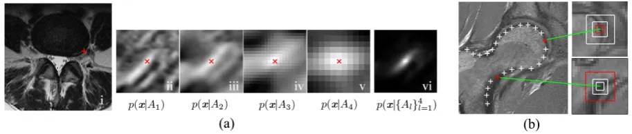
Figure 2: (a) i: A marked feature point (red cross); ii to v: Response maps from four level local features in a LFP at the landmark. Red crosses denote the true locations. The smaller scales are plagued by the problem of ambiguity, while the lager scales have low spatial specificity; vi: A product combination of the response maps, which enhances the specificity and suppresses the ambiguity. (b) Local features are salient at certain scales. A LFP is able to preserve the salient scales (red rectangles).

1. Resistance to local minima, see Fig. 2(a). Local feature detectors are plagued

by the problem of ambiguity. This ambiguity is evident in the distribution of

landmark locations (i.e., the response map) obtained from a feature detector, see Fig. 2(a: ii). [12] use a multi-scale parametrisation of the response map to seek for the true position. The feature pyramid however, deals with this problem from a different perspective: it calculates multi-scale response maps (see Fig. 2(a: i to iv)) from multi-scale patches, and combines the responses to deduce the true position. The larger scale ensures a wider support range while the small scale yields a high precision.

2. Enhanced distinctive ability, see Fig. 2(b). Local features are salient at certain scales, and the salient scale can vary across the landmarks. As noted earlier, a single-scale descriptor will either be too small to capture the texture or too spread-out to give its precise location. In comparison, the feature pyramid can preserve the salient features at whatever scales it appears (e.g., the red patches in Fig. 2(b)).

3.2

Active appearance pyramid

Figure 3: (a) Image with landmarks. (b) AAP with 4 level feature pyramids. (c) The

AAP delineation. (d) Concatenated LFPs form a 1D AAP vector A.

An AAP is a part-based model with each part delineated by a LFP. The AAP consists

of two elements: {A,s}, with A being the assembly of the feature pyramids and s

patches at landmark intervals at the larger scales. The principle of trimming is to obtain an even coverage of the appearance at each level, see Fig. 3(b). In practice, a simple trimming algorithm can be designed to iteratively delete the landmark who has least distance from its neighbourhood until a distance criterion is matched. Alternatively the landmark to preserve can be selected by hand to highlight the anatomical features of

interest. Denoting Kl as a subset of natural numbers{1, ..., N} indicates the landmarks

preserved at the l-th scale. The assembly of the trimmed parts can be denoted as A =

{{Ai,l}i∈Kl} L

l=1, see Fig. 3(d) for the example. Ais then flattened into a 1D vector serving

as the profile of the whole object appearance.

Given the training set we can extract anAfrom each image and obtain a set of training

data {A1,A2, ...}. By extracting the local features from the corresponding landmarks,

the shape variation in the training set has already been removed and a better

pixel-to-pixel correspondence achieved, therefore A can be viewed as ‘shape-free’ appearances

and an extra image warping as necessary in AAMs is avoided. It should be noted that at larger scales, the structural deformation might be included. However this is acceptable because larger scales have lower resolution and therefore are less sensitive to the shape

variations. A can be visualised by recovering the dimension and location of each feature

patch, padding and placing smaller scale patches on top of larger ones, see Fig. 3(c). To obtain a statistical model of the shape-free appearance, we normalise the mean and

variance of each A and apply PCA on the training samples. A new instance can be

linearly modelled by,

A= ¯A+PAbA, (3)

in which ¯A is the mean, PA spans the eigenspace and bA is the appearance parameters

in the subspace.

4

Active appearance pyramid fitting

The AAP is parametrised by the appearance of the assembly of parts as well as the shape capturing spatial relationships. It therefore fits and synthesises new instance by adjusting

global appearance parameter bA, and estimating local translations for individual patches

with a regulariser imposed on the shape s. We follow the two-step fitting strategy

com-monly used in part-based models, i.e, local feature searching followed by a geometrical regularisation.

4.1

LK based simultaneous local feature searching and

appear-ance fitting

The LK algorithm attempts to find the parameters p to minimise the difference between

a template T and a source image J,

p = arg min||J(p)−T||2, (4)

where p can be image translation or warping. To enhance the robustness and efficiency

respectively, two extensions have been made, namely weighted LK and inverse gradient descent [31]. The weighted LK can be posed as,

p = arg min||J(p)−T||2

whereQis the weighting matrix usually representing a linear transform such as a subspace projection in the AAMs [4], weighted subspace projection [32], or Gabor filtering in the Fourier LK [33, 34].

We derive a subspace LK for the AAP fitting, with a further simplification by applying the conditional independence assumption of the part-based models. Specifically, the dif-ference between the template and the textures it covers can be caused by the appearance variation of the object and the departure of the model to the true position. Accordingly

they can be dealt with in two subspaces: the eigen-space span(PA) accounting for the

appearance variation and its orthogonal space span(PA)⊥ to predict the landmark shift.

The appearance parameters bA can be calculated by projecting A onto the eigenspace,

bA =PAT(A(s)−A¯). (6)

bA only need to be calculated once after the shape fitting has converged. The landmarks

are predicted by implementing the LK algorithm in the orthogonal space,

ˆ

s = arg min||A(s)−A||¯ 2

span(PA)= arg min||(A(s)−

¯

A)⊥||2_{, (7)}

where (·)⊥ denotes the projection onto the orthogonal space, i.e., (·)⊥ = (I −PAPAT)(·),

with I being an identity matrix. In this way the salient appearance variations have

been removed and a more robust LK method achieved. Equation (7) can be solved by iteratively linearising and inverse gradient descent by reversing the roles of the image and template [35],

∆ˆs = arg min||A¯⊥(∆s)− A⊥(s)||2_{. (8)}

We apply the conditional independence assumption to simplify the calculation, i.e.

the patches at the i-th landmark are only related to xi, therefore the equation can be

decomposed into a set of independent equations,

∆ ˆxi,l= arg min ¯A⊥i,l(∆xi)−A⊥i,l(xi)

. i∈ {1, ...N}, l∈`i (9)

where Ai,l is the feature patch at i-the landmark with l-th scale, flattened into a 1D

vector. ∆ ˆxi,l is the predicted increment of the i-th landmark inferred from Ai,l. The

solution is given by a least squares method,

∆ ˆxi,l =

∂A¯⊥_i,l

∂xi

!+

(Ai,l(xi)−A¯i,l)⊥, (10)

in which (·)+ denotes the Moore-Penrose pseudo-inverse. Inside the bracket of the first

factor is the gradient map of the mean patch at thei-th landmark andl-th scale, projected

onto the orthogonal space.

Suppose we also have the variance σ_i,l2 of the prediction ∆ ˆxi,l, which could indicate

the salience of the feature or the confidence of the prediction. To keep it simple, we calculate the variance as the mean squared difference between the patch observation and the template. Using a Gaussian parametric form and applying the product combination

in (2), the likelihood of the location of thei-th landmark given the multi-scale predictions

can be represented by,

p(xi|{Ai,l}l) =

Y

l

N(xi; ˆxi,l,σi,l2), (11)

where ˆxi,l are the updated landmark estimated by adding ∆ ˆxi,l to the current location.

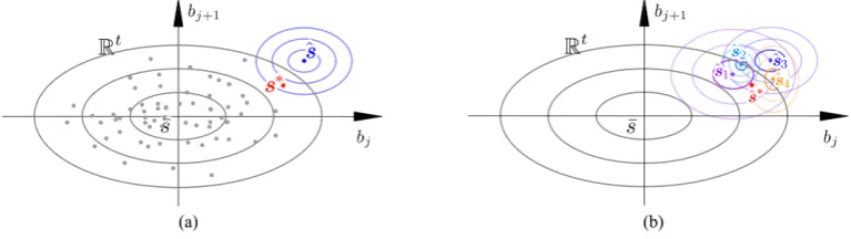
Figure 4: (a) An illustration of shape inference in the eigenspace spanned by P ∈ _Rt_. Grey dots represent the training samples, ellipses show the three standard deviations of the Gaussian distribution which gives the prior knowledge of shapes. The shape

observa-tions ˆs are shown in blue, with the variance representing the confidence. The ML shape

s∗ is inferred from the prior and the observation. (b) ML shape inferred from the prior

(grey) and multiple observations ˆsi. Ellipses show three standard deviations. The ML

shapes∗ is inferred seeking a balance between the prior and the observations.

4.2

Shape regularisation

The shape can be either bounded by a subspace constraint [36] as in standard ASMs or optimised by a regulariser using, e.g., density estimation [26, 37], a Bayesian model [11], or sparse shape composition [38, 39], leading to more efficient fitting. It has been shown that utilising multiple predictions of individual landmarks can result in robust fitting. For example, in [40] multiple candidates at a landmark are generated, then the best one is selected and the others are regarded as false positives. There have been multi-scale shape models [41, 42] to characterise the population variations in a more accurate and robust way. To keep our method simple, we show how a standard Gaussian shape model can be integrated with multi-scale landmark predictions

We assume that all of the multi-scale predictions from LFPs are valid, but with various weights across the landmarks and scales controlled by their variances, and deduce a regulariser to obtain the ML shape with respect to the shape prior and the multi-scale landmark predictions. Specifically, the likelihood of a shape instance given the shape

prior Ω and image observation I can be represented as p(s|Ω, I). Since Ω and I are

conditionally independent, from Bayesian theory we have,

p(s|Ω, I)∝p(s|Ω)p(s|I). (12)

Assuming the shape parameters b are Gaussian distributed across the population, the

prior factor can be written as,

p(s|Ω)∝

t Y

j=1

exp

_−b2

j 2λj

, (13)

in which bj is the j-th element and t is the dimension of b.

In an AAP we obtain shape observations from multiple scales, and at each scale a subset of landmarks is estimated. In order to infer the optimal shape from this

infor-mation, we first consider the two following questions: (1) At a certain level l, given the

observation of a subset of landmarks inKl, how to deduce the whole shape based on the

Inferring the whole shape from a subset of landmark estimations. At a

single scale l of a trimmed AAP, we can only obtain the estimations of a subset of

‘key’ landmarks, ˆxi, i ∈ Kl with variances {σ2i}. To estimate the whole shape from

this information, the remaining ‘empty’ landmarks can be inferred based on the key landmarks and the shape prior. Specifically, as we have no observation of the empty landmarks, their likelihood can be modelled as a Gaussian with infinite variance, which assumes all locations are equally likely. In this way we can write the likelihood for all

landmarks observed from scale l as,

p(xi|I) =

(

N( ˆxi,l, σ2i,l), i∈ Kl

N(0,Inf) i6∈ Kl.

(14)

Accordingly the shape observation becomes,

p(s|I) =

N X

i=1

p(xi|I). (15)

Substituting (15) into (12) and taking the negative log form we can obtain an energy function,

E(s) =

t X

j=1

b2_j

2λj

+ N X

i=1

(xi−xˆi,l)2

2σ2

i,l

. (16)

where ˆxi,l takes the value zero and σi,l2 infinite at empty landmarks. The ML shape

in-ferred from a single scale observation can be calculated by minimising the energy function. The resulting shape is the one best fitting the prior and the key landmarks. Fig. 4(a) gives an illustration of ML shape inference in the eigen-space.

Inferring the ML shape from multiple shape observations. Given multiple

shape observations ˆsi the likelihood of the shape can be formularised as a product,

p(s|I) =

L Y

l=1

pl(s|I) =

L Y l=1 N Y i=1

N(xi; ˆxi,l,σ2i,l) (17)

Substituting (13) and (17) into (12) and taking the negative log form, the new energy function obtained is,

E(s) =

t X j=1 b2 j 2λj + L X l=1 N X i=1

(xi−xˆi,l)2

2σ2_i,l . (18)

The shape minimising (18) is the ML shape with respect to the prior and all the landmark observations available. It seeks an optimal solution balanced between the prior and the observations, the weights of which is determined by the confidence of observations, see Fig. 4(b) for an illustration.

In practice a weighting parameter is added to balance the shape prior and the feature observation giving greater control, and the equation becomes,

E(s) =

t X

j=1

b2_j

2λj +β L X l=1 N X i=1

(xi−xˆi,l)2 2σ2

i,l

Instead of numerical optimisation, observing the homogeneous form of the equation, we derive a closed-form solution, (see Appendix 1):

s = (PΛ−1PT +β L X

l=1

Σ−_l 1)−1(PΛ−1PTs¯+β L X

L=1

Σ−_l1ˆsl), (20)

where Λ = diag([λ1, ..., λt]) and Σl = diag([σ12,l, ...,σN,l2 ]). The value of β is set to 1 in

our experiments.

4.3

Reconstruction of the object appearance

As the shape of the object is fitted using the method presented above and the

appear-ance is encoded in the parameters bA, we can recover the object information from the

parameters. The reconstructed object can be visualised by first recovering the ‘shape-free’

appearanceA by (3) and then padding the multi-scale patches inA at the corresponding

position, with the smaller scales layered on top of larger ones.

The implementation of the whole algorithm is outlined in Algorithm 1.

Algorithm 1: Active Appearance Pyramid fitting

Training

1. Train the shape prior, obtain the mean shape ¯s, the eigenvalues {λj}t

j=1 and the

eigenvector matrixP;

2. Build the Gaussian pyramid of training data and extract the training AAPs{A};

3. Train the appearance prior on {A}, obtain the mean ¯Aand the eigenvector matrix

PA;

4. Calculate the mean in orthogonal space ¯A⊥ _{and the gradient of each patch in ¯A}⊥_,

i.e.,∂A¯⊥_i,l/∂xi, i∈ {1, ...N}, l∈`i. Testing

1. Build the Gaussian pyramid of the testing image, initialise the shape s;

2. Extract the AAP A(s) at the current shape;

3. Local searching: ProjectA(s) onto the orthogonal space, calculate the multi-scale

landmark predictions by (10);

4. Regularisation: Calculate the ML shapes by (20);

5. Repeat 2 to 4 until the shape converged;

6. Calculate the appearance parametersbA using (6).

7. (Optional) reconstruct the object appearance froms andbA.

5

Experiments and results

femoroacetabular impingement. We comparatively assess the computational cost against AAM, the mean surface errors and the reconstruction quality.

5.1

2D experiments on the lumbar vertebral images

Figure 5: Disc-level axial images and parasagittal images. (a) Anatomy of a normal L3/4 axial image. (b) Foraminal stenosis. The neural foramen and the central canal are suppressed by the thickening facet (green circle) and the disc (red line). (c) Central canal narrowing caused by disc herniation in green circle area. (d) Parasagittal image of a normal case (left) and one with stenosis (right). Red circles outline the neural foramen.

5.1.1 Clinical background

foraminal stenosis. An example with foraminal stenosis is given in Fig. 5(b), in which the neural foramen is constricted by the thickening of the facet (green circle area) and the posterior margin of the disc. Fig. 5(c) shows a case of central narrowing caused by a disc herniation. In parasagittal images, the nerve foramen (Fig. 5(d) red contours) are inspected to assess foraminal stenosis. In clinical practice, parameters such as antero-posterior diameter, cross-sectional area of spinal canal on axial images and foraminal diameter on parasagittal images are typically used to quantify the severity of LSS [43]. However there is a lack of consensus in the literature and no diagnostic criteria are generally accepted [44]. As the pathologies exhibited in different areas are usually related, a more specific parametrisation and fitting of the structure, followed by a higher-level classification could contribute to more reliable, consistent and accurate diagnoses.

5.1.2 Validation

Data. The clinical data consists of axial and sagittal T2-weighted MRI scans of 200

patients with varied LSS symptoms. Each patient has routine anisotropic axial and sagittal scans. From the axial scans we obtain a dataset of 200 disc-level axial images on each of the three intervertebral cross-sections, with the features of interest expertly annotated with 37 landmarks. From the sagittal scans we extracted 400 parasagittal images (200 on each side) around L3/4, L4/5 and L5/S1 nerve foramina respectively. The contour of each foramen is annotated by 13 landmarks. The annotated data are used for the training as well as serving as the ground truth.

Parametrisation. For axial images, the AAP is built with four level feature pyramids

(see Fig. 3(b)). The patch size is 15×15 pixels. Similarly, for parasagittal images we use

a three level AAP with the patch size of 9×9 pixels.

In order to visualise the statistical variation among the population caused by LSS,

we concatenate the appearance parameters bA and shape parameters b appropriately

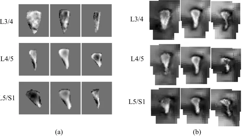
weighted for an equivalent variance. PCA is then applied to obtain the joint model. Fig. 6 shows the mean and the most significant variation of axial intervertebral anatomies L3/4 and L5/S1. Fig. 7 gives the mean and the first variation of the three intervertebral foramina. The first mode obtained by standard AAM reconstruction is also given in these cases for comparison. We can see that the AAP preserves more delicate features and richer information.

Cross-fold validation. For each of the three axial datasets we randomly pick 40

samples as training data and test the methods on the remaining 160, and repeat for several times for an unbiased validation. Similarly for each of the 3 parasagittal dataset we randomly pick 40 samples for the training and test the methods on the remaining 360 and repeat.

Two measurement criteria are used for the evaluation: the Point to Boundary Distance (PtoBD) in pixels and the Dice Similarity Coefficients (DSC) [45]. DSC is defined as the amount of the intersection between a segmented object and the ground truth, DSC =

2·TP/(2·TP + FP + FN), with TP, FP, FN denoting the true positive, false positive

and false negative values respectively. For the axial images, the DSC of the canal and disc contours between the fitted shape and the ground truth is used as the criterion of segmentation precision.

Figure 6: First mode of variation across the population with varied LSS, generated by

(a) AAM and (b) AAP. Shown are the average appearance (middle) and the ±2 SD

variation. Images are shown at the same scale. The AAP preserves more delicate texture of important features and covers a larger context region.

5.1.3 Results

Convergence range. We run displacement experiments on the axial images to test

Figure 7: First mode of the variation of the three foramina generated by (a) AAM and

(b) AAP. Shown are the mean (middle) and the ±2 SD variation. Images are shown at

the same scale.

0 10 20 30 40

Initial Displacement (pixels) 0 0.2 0.4 0.6 0.8 1 Convergence Rate AAM ASM CLM AAP (a) L3/4

0 10 20 30 40

Initial Displacement (pixels) 0 0.2 0.4 0.6 0.8 1 Convergence Rate AAM ASM CLM AAP (b) L4/5

0 10 20 30 40

Initial Displacement (pixels) 0 0.2 0.4 0.6 0.8 1 Convergence Rate AAM ASM CLM AAP (c) L5/S1

0 10 20 30 40

Initial Displacement (pixels) 0 0.2 0.4 0.6 0.8 1 Convergence Rate AAM+ ASM+ CLM+ AAP (d) L3/4

0 10 20 30 40

Initial Displacement (pixels) 0 0.2 0.4 0.6 0.8 1 Convergence Rate AAM+ ASM+ CLM+ AAP (e) L4/5

0 10 20 30 40

Initial Displacement (pixels) 0 0.2 0.4 0.6 0.8 1 Convergence Rate AAM+ ASM+ CLM+ AAP (f) L5/S1

Figure 8: Successful convergence rate of compared methods on lumbar intervertebral slices L3/4, L4/5 and L5/S1. Top row: comparison with the single scale methods. Bottom

row: comparison with the coarse-to-fine version of these methods (denoted by (·)+). AAP

shows a significant superior performance in convergence range against all three methods, as well as robustness against the coarse-to-fine implementation of these methods.

displacement, which means in low quality or challenging cases, the shape could diverge at the coarse level because of lack of texture details. This further support our argument of combining multi-scale features to enhance the robustness. The improvement of AAP is on account of the multi-scale LFPs. The larger scales ensure a wider capture range, while the smaller scales take effect as soon as it gets into the convergence range.

Precision of segmentation. For each testing case, the shape is initialised as the

Number of scales

1 2 3 4

Error 1.9 2 2.1 2.2 2.3 2.4 2.5 _L3 L4 L5

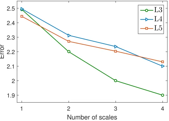
Figure 9: Fitting error against the number of scales used in AAP.

0 1 2 3 4 5 6 Point to Boundary Distance 0 0.2 0.4 0.6 0.8 1

Cumulative Error Distribution

AAM: 2.81±1.27 ASM: 2.30_±1.35 CLM: 2.10±0.96 AAP:1

.84±0.80

(a) L3/4

0 1 2 3 4 5 6 Point to Boundary Distance 0 0.2 0.4 0.6 0.8 1

Cumulative Error Distribution

AAM: 3.04±1.23 ASM: 2.53_±1.33 CLM: 2.43±1.37

AAP:2

.00±0.90

(b) L4/5

0 1 2 3 4 5 6 Point to Boundary Distance 0 0.2 0.4 0.6 0.8 1

Cumulative Error Distribution

AAM: 3.05±1.07 ASM: 2.59_±1.16 CLM: 2.70±1.16 AAP:2

.13±0.83

(c) L5/S1 0.8 0.85 0.9 0.95 1

Dice Similarity Coefficient

0 0.2 0.4 0.6 0.8 1

Cumulative Error Distribution

AAM: 91.5_±4.6 ASM: 93.0±5.3 CLM: 93.6±3.4 AAP:94

.5±2.8

(d) L3/4 0.8 0.85 0.9 0.95 1

Dice Similarity Coefficient

0 0.2 0.4 0.6 0.8 1

Cumulative Error Distribution

AAM: 91.4_±4.3 ASM: 92.5±4.5 CLM: 93.3±4.1 AAP:94

.5±2.9

(e) L4/5 0.8 0.85 0.9 0.95 1

Dice Similarity Coefficient

0 0.2 0.4 0.6 0.8 1

Cumulative Error Distribution

AAM: 91.6_±4.7 ASM: 92.1±4.9 CLM: 92.3±3.6 AAP:94

.5±2.3

(f) L5/S1

Figure 10: Cumulative error distribution of segmentation of lumbar intervertebral slices: L3/4, L4/5 and L5/S1. DSC and PtoBD (in pixels) are used as the criteria. Compared methods are AAM, ASM, CLM and AAP. The legends give the mean errors and standard deviations

To demonstrate the benefit of using the multi-scale local feature pyramids as feature descriptor, we report the performance of AAP with different number of scales in Fig. 9. We can see that in all three subsets the fitting error reduces with the increasing number of scales utilised.

Due to the higher failure rate of the coarse-to-fine approaches even at small initial displacements (as shown in Fig. 8), we only compare the precision of our AAP with the single scale implementation of these methods, and set the initial displacement small enough to keep them within a confident convergence range. The algorithms are then applied to fit the shape to the image. We repeat the process several times for an unbiased result. The cumulative error distribution of the DSC and PtoBD of the segmentation results on three axial dataset are shown in Fig. 10. The mean error and one standard deviation (SD) is also given in the legends for the comparison. We can see that AAP achieves the best precision of segmentation. Meanwhile the smaller SD shows that AAP has the superior consistent performance, which is also indicated in the cumulative error distribution curves. For example, the proportion of the segmentation results with PtoBD smaller than four pixels is (97%, 97%, 96%) with AAP on three dataset respectively (see Fig. 10(b)(d)(f)) , while the proportion is only (95%, 92%, 87%), (91%, 89%, 87%) and (86%, 80%, 85%) with CLM, ASM and AAM respectively.

The qualitative results of segmentation on five representative cases are shown in Fig. 11, with the difficulty increasing from left to right. The ground truth shape is shown in each case for convenience. We can see that the AAMs, ASMs and CLMs are affected by local ambiguity (highlighted by red circles) on the challenging cases and become trapped in a local minimum. We observe large proportion of outliers by AAM around the disc like the third case in Fig. 12. A possible reason is that the plain textures inside the disc contain very limited information. The AAPs shows a robust and consistent performance in all five cases.

Comparisons of object reconstruction. As the parameters of AAM and AAP

encode both the shape and appearance information, we can reconstruct the anatomy from the fitted parameters. In addition to morphometric comparison, the quality of appearance synthesis can indicate how precise the object is modelled and appearance details are represented. We therefore quantify and compare the appearance fitting quality using the image distortion as a measurement. We calculate the error map of a synthesised appearance as follow,

Err(x) = [I(x)−J(x)]

2

[I(x)]2 . (21)

whereI is the true image andJ is the synthesised result. The synthesised appearance as

well as the error map for five cases by AAM and AAP are shown in Fig. 12. We can see that AAP preserves more dedicate structural details and covers larger area of contextual information. For example, the facet is precisely located and the facet texture is well preserved in all five cases. In case three and four, the AAP delineates the degenerated vertebrae and the compressed central canal more accurately than AAM does. The large errors of AAM are mainly distributed around the feature of interest where the pathology might appear. We also evaluate the overall synthesis error of a case by calculating the signal-to-noise ratio (SNR),

SNR = E[I(x)]

2

E[I(x)−J(x)]2, x ∈Ω, (22)

Figure 11: Segmentation results on five cases, increasing in difficulty from left to right. The ground truth of segmentation is shown by yellow dash lines, fitting results are shown by cyan crosses. Red circles highlight the outliers.

means and SD of the SNR of the testing samples are reported in Table. 1. We can see that compared with the shape fitting results, the improvement in appearance fitting by AAP is more significant.

Table 1: Means and SD of SNR of synthesised results by AAM and AAP.

L3/4

L4/5

L5/S1

AAM

4.80

±

2.73

5.36

±

2.60

7.51

±

5.06

AAP

8.72

±

4.71

6.96

±

3.77

9.38

±

4.71

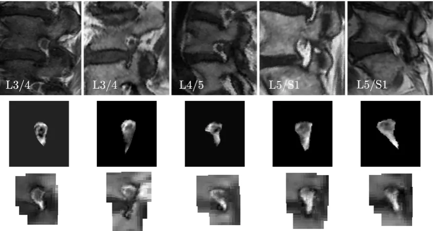
Reconstruction of neural foreman. We also report the qualitative results of

Figure 12: Reconstruction results on five cases, increasing in difficulty from left to right. The reconstructed appearances are the parametric models with the parameters fitted to

the instances.2 _{The error maps highlight the regions with low fitting precision, which are}

mainly around the features of interest.

5.2

Segmentation and reconstruction of 3D hip joint data

5.2.1 Data

We apply the 3D AAP on the parametrisation and segmentation of the hip joint in CT of patients with femoroacetabular impingement. The data are pre-interpolated to obtain an isotropic voxel size of 1 mm. The femoral head and acetabulum are annotated by 427 and 254 points marked up by experts. We build two AAP models delineating these two anatomies respectively. Both models are composed of four-level cubic patches with

a consistent size of 9×9×9 voxels. A cross validation is performed on 38 CT volumes,

i.e., randomly picking 19 samples as training data, and testing on the remainder, and repeating.

2_{As the object appearance is synthesised and parametrised, we can animate the progress of anatomical}

Figure 13: Fitting and reconstruction results of neural foramen on five cases. Top: Testing data; Middle: Reconstructed appearance by AAMs; Bottom: Reconstructed appearance by AAPs.

5.2.2 Computational efficiency

The AAP model parametrising the femoral head consists of 617 patches with size of nine-voxels cubed, which is 449,793 nine-voxels for each instance. As a comparison, the AAM uses

a 92×96×96 volume which consists of 847,872 voxels. Thus the AAP uses 53% of voxels

compared with the AAM, while covering a much larger contextual region and preserving a full resolution of the features of interest such as the articular surface. Similarly, a second acetabulum model uses 58% voxels of the AAM does.

We tested the time consumed by the AAM and AAP for training and fitting using a quad-core 3.2GHz processor with 16GB memory. Both algorithms were implemented in MATLAB, with the intensive computations of the AAM compiled in C++ language to boost its performance. We observe that it takes 170 ms to generate a shape-free appearance of femoral head by warping the volume, after compilation in C++. As a comparison, the most intensive computation of AAP, i.e., to generate the Appearance Pyramid by extracting subvolumes from the data, takes only 40 ms in MATLAB. We report the time consumed by each principal task on the femoral head data in Table 2. We can see that the AAP consumes less than 10% the training time and 15% the testing time of the AAM.

5.2.3 Precision of segmentation and reconstruction

Figure 14: (a) The mean shape of the acetabulum (red) and femoral head (blue). (b) The mean appearance of the two anatomies generated by AAM (top) and AAP (bottom).

Table 2: Time consumption of AAM and AAP on femoral head

Process AAM AAP

Loading data: 18.0 s 18.0 s

Training: Build gaussian

pyramids:

45.8 s

9.8 min AAP training: 7.4 s

Total: 53.2s

Fitting (30 iterations): 18.3 s 2.7s

Reconstruction: 0.6 s 0.3s

AAM AAP

2

1

0 voxels

1.06±0.41 voxels 0.96±0.60 voxels 0.79±0.26 voxels 0.74±0.25 voxels

Figure 15: Mean vertex-to-surface errors of the segmentation results of the acetabulum and femur head, displayed on the mean shape mesh. The mean errors and standard deviations are shown at the bottom.

head. In addition, the smaller SD indicates the robustness of AAP across the cases.

Figure 16: Qualitative results of the reconstruction. Shown are the testing data (left), and the appearance modelled and fitted by AAM (middle) and AAP (right).

Figure 17: Qualitative results of the reconstruction. Shown are the testing data (a), and the appearance modelled and fitted by (b) AAM and (c) AAP. The volumes are shown with paired axial and coronal cross-sections.

cross-sections in Fig. 17 to give a clearer view.3 _{Anatomies in each figure are shown in the same}

size ratio. The AAP syntheses cover a larger contextual region, which is why they appear to be larger. We can see that the AAP preserves sharper and more precise structures. Whereas in the AAM the reconstruction is blurred and with noticeable distortion.

6

Conclusions

We presented a part-based appearance model we refer to as an AAP. A simultaneous landmarks searching and appearance fitting algorithm was derived based on the weighted Lucas and Kanade method. We introduced a shape regulariser utilising multi-level land-mark estimation, and derive a closed-form solution to the maximum likelihood shape. The AAP can parametrise an object class and synthesise new instances as an AAM does. However the AAP differs from holistic AAMs in two respects: (i) AAMs model intra-class variations with local affine transforms, while AAPs approximate the deformation with local translations of multi-scale parts; (ii) AAMs model the inner region of the shape mesh while AAPs cover the contextual information with multiple resolutions. We ran experiments to validate its performance and highlighted its advantages in several respects:

1. Computational efficiency. Computational cost has been a main limitation in existing appearance models tackling volume data. Compared with the AAMs, an AAP keeps full resolution of salient features, with reducing resolution further away from landmarks, which covers larger context but consumes less memory. AAP training and fitting is much faster because no image warping or interpolation is needed. The time consumption for both training and testing is linear to the number of samples in the dataset, so we can expect a time saving of 10% / 15% in training / testing correspondingly for large datasets. It also has a simpler form and is easier to implement.

2. Fitting precision and robustness. The AAP spreads outside the shape mesh and captures more contextual information. Compared with AAMs and CLMs, the multi-scale feature descriptors enhance both position specificity and textural distinguish-ing ability, result in a superior fittdistinguish-ing precision and robustness to local minima. The larger convergence range also makes it more robust to initialisation.

3. Precision of parametrisation and reconstruction. We observe a more delicate and precise reconstruction result in AAP. The better quality of reconstruction indicates two facts. Firstly, it captures and utilises more precise object appearance for shape fitting, which is demonstrated by its better segmentation performance. Secondly, it indicates that the more delicate and richer appearance is parametrised and encoded in the AAP parameters. As a result, it should contribute improved performance for the subsequent diagnostic tasks.

Our possible further work will involve the use of a more sophisticated shape prior such as sparse shape composition [39] and Independent Component Analysis [46], and investigating into integrating them with multiple landmark candidates from LFP. For the study of LSS, we are designing and testing classification algorithms based on the AAP

3_{Videos and DICOM files of the 3D results are available online at}

delineation. It has been shown in literature that combining shape and local features in CLM can result in a robust classification in clinical tasks [46]. As the AAP achieves a higher precision and gives a more delicate and unbiased delineation, we expect it could contribute to a practical LSS diagnosis and grading system.

A

Derivation of the closed-form solution to the

op-timal shape

The maximum likelihood shape is the one minimising the energy function,

E(s) =

t X j=1 b2 j 2λj +β N X i=1 L X l=1

(xi−xˆi,l)2 2σ2

i,l

, (23)

which can be rewritten in a matrix form,

E(s) = 1

2b

T

Λ−1b+ 1

2β

L X

l=1

(s−sˆl)TΣl−1(s−sˆl), (24)

where Λ = diag([λ1, ..., λt]) and Σl = diag([σ21,l, ...,σN,l2 ]), b is the vector of shape

pa-rameters ands is the shape. Equation 24 has the typical form of an energy function for

shape regularisation, with the notable difference that the second term is a summation of multiple predictions. Substituting (1) into (24) gives,

E(s) = 1

2(s−s¯)

T_PΛ−1_PT_{(s−s¯) +} 1

2β

L X

l=1

(s −ˆsl)TΣl−1(s−sˆl). (25)

The optimal value of s is the one minimising E(s), obtained by solving the equation:

dE(s)

ds =PΛ

−1_PT_{(s−s¯) +β} L X

l=1

Σ−_l 1(s−sˆl) = 0. (26)

The solution is,

s = (PΛ−1PT +β L X

l=1

Σ−_l 1)−1(PΛ−1PTs¯+β L X

l=1

References

[1] Michael J Jones and Tomaso Poggio. Multidimensional morphable models: A

frame-work for representing and matching object classes. International Journal of

Com-puter Vision, 29(2):107–131, 1998.

[2] Daniel Rueckert, Alejandro F Frangi, Julia Schnabel, et al. Automatic construction

of 3-D statistical deformation models of the brain using nonrigid registration. IEEE

Transactions on Medical Imaging, 22(8):1014–1025, 2003.

[3] Timothy F Cootes, Gareth J Edwards, and Christopher J Taylor. Active

appear-ance models. IEEE Transactions on Pattern Analysis and Machine Intelligence,

23(6):681–685, 2001.

[4] Iain Matthews and Simon Baker. Active appearance models revisited. International

Journal of Computer Vision, 60(2):135–164, 2004.

[5] Martin Roberts, Timothy F Cootes, and Judith E Adams. Vertebral morphometry: semiautomatic determination of detailed shape from dual-energy X-ray

absorptiom-etry images using active appearance models. Investigative radiology, 41(12):849–859,

2006.

[6] Martin G Roberts. Automatic detection and classification of vertebral fracture using

statistical models of appearance. PhD thesis, University of Manchester, 2008.

[7] Pedro F Felzenszwalb and Daniel P Huttenlocher. Pictorial structures for object

recognition. International Journal of Computer Vision, 61(1):55–79, 2005.

[8] Pedro F Felzenszwalb, Ross B Girshick, and David McAllester. Cascade object

detection with deformable part models. In 2010 IEEE Conference on Computer

Vision and Pattern Recognition, pages 2241–2248. IEEE, 2010.

[9] P. F. Felzenszwalb, R. B. Girshick, D. McAllester, and D. Ramanan. Object detection

with discriminatively trained part-based models. IEEE Transactions on Pattern

Analysis and Machine Intelligence, 32(9):1627–1645, 2010.

[10] David Cristinacce and Timothy F Cootes. Feature Detection and Tracking with

Constrained Local Models. InProceedings of the British machine Vision Conference,

volume 1, page 3. Citeseer, 2006.

[11] David Cristinacce and Tim Cootes. Automatic feature localisation with constrained

local models. Pattern Recognition, 41(10):3054–3067, 2008.

[12] Jason M Saragih, Simon Lucey, and Jeffrey F Cohn. Deformable model fitting

by regularized landmark mean-shift. International Journal of Computer Vision,

91(2):200–215, 2011.

[13] Xiangxin Zhu and Deva Ramanan. Face detection, pose estimation, and landmark

localization in the wild. In IEEE Conference on Computer Vision and Pattern

[14] Claudia Lindner, S Thiagarajah, J Wilkinson, The Consortium, G Wallis, and Tim-othy F Cootes. Fully automatic segmentation of the proximal femur using random

forest regression voting. Medical Imaging, IEEE Transactions on, 32(8):1462–1472,

2013.

[15] David Cristinacce and Timothy F Cootes. Boosted Regression Active Shape Models.

In BMVC, pages 1–10, 2007.

[16] Jason M Saragih, Simon Lucey, and Jeffrey F Cohn. Face alignment through

sub-space constrained mean-shifts. InIEEE 12th International Conference on Computer

Vision, pages 1034–1041. IEEE, 2009.

[17] Epameinondas Antonakos, Joan Alabort-i Medina, and Stefanos Zafeiriou. Active

Pictorial Structures. In Proceedings of the IEEE Conference on Computer Vision

and Pattern Recognition, pages 5435–5444, 2015.

[18] Xuehan Xiong and Fernando De la Torre. Supervised descent method and its

ap-plications to face alignment. InComputer Vision and Pattern Recognition (CVPR),

2013 IEEE Conference on, pages 532–539. IEEE, 2013.

[19] Bruce D Lucas, Takeo Kanade, et al. An iterative image registration technique

with an application to stereo vision. In International Joint Conference on Artificial

Intelligence, volume 81, pages 674–679, 1981.

[20] Nuria Brunet, Francisco Perez, and Fernando De La Torre. Learning good features

for active shape models. In Computer Vision Workshops (ICCV Workshops), 2009

IEEE 12th International Conference on, pages 206–211. IEEE, 2009.

[21] Martin G Roberts, Tim F Cootes, Elisa Pacheco, Teik Oh, and Judith E Adams. Segmentation of lumbar vertebrae using part-based graphs and active appearance

models. InMedical Image Computing and Computer-Assisted Intervention–MICCAI

2009, pages 1017–1024. Springer, 2009.

[22] Philip A Tresadern, Harish Bhaskar, Steve A Adeshina, Christopher J Taylor, and Timothy F Cootes. Combining Local and Global Shape Models for Deformable

Ob-ject Matching. In Proceedings of the British Machine Vision Conference, volume 9,

pages 451–458, 2009.

[23] Mikkel B Stegmann. Generative interpretation of medical images. Lingby: Thesis,

University of Denmark, 2004.

[24] Steven C Mitchell, Johan G Bosch, Boudewijn PF Lelieveldt, Rob J van der Geest, Johan HC Reiber, and Milan Sonka. 3-D active appearance models: segmentation

of cardiac MR and ultrasound images. IEEE Transactions on Medical Imaging,

21(9):1167–1178, 2002.

[25] Alexander Andreopoulos and John K Tsotsos. Efficient and generalizable statistical

models of shape and appearance for analysis of cardiac MRI.Medical Image Analysis,

12(3):335–357, 2008.

[26] Matthias Kirschner, Meike Becker, and Stefan Wesarg. 3D active shape model

seg-mentation with nonlinear shape priors. InMedical Image Computing and

[27] Roland Wilson and Michael Spann. Image segmentation and uncertainty. John Wiley & Sons, Inc., 1988.

[28] Cormac Herley, Jelena Kovacevic, Kannan Ramchandran, and Martin Vetterli. Tilings of the time-frequency plane: Construction of arbitrary orthogonal bases and

fast tiling algorithms. IEEE Transactions on Signal Processing, 41(12):3341–3359,

1993.

[29] Lorenzo Seidenari, Giovanni Serra, Andrew D Bagdanov, and Alberto Del Bimbo.

Local pyramidal descriptors for image recognition. Pattern Analysis and Machine

Intelligence, IEEE Transactions on, 36(5):1033–1040, 2014.

[30] Jingming Dong and Stefano Soatto. Domain-size pooling in local descriptors:

DSP-SIFT. arXiv preprint arXiv:1412.8556, 2014.

[31] Simon Baker and Iain Matthews. Equivalence and efficiency of image alignment

algo-rithms. InProceedings of the 2001 IEEE Computer Society Conference on Computer

Vision and Pattern Recognition, volume 1, pages I–1090. IEEE, 2001.

[32] Minh Hoai Nguyen and Fernando De La Torre. Local minima free parameterized

appearance models. In 2008 IEEE Conference on Computer Vision and Pattern

Recognition, pages 1–8. IEEE, 2008.

[33] Ahmed Bilal Ashraf, Simon Lucey, and Tsuhan Chen. Fast image alignment in

the fourier domain. In 2010 IEEE Conference on Computer Vision and Pattern

Recognition, pages 2480–2487. IEEE, 2010.

[34] Rajitha Navarathna, Sridha Sridharan, and Simon Lucey. Fourier active appearance

models. In 2011 IEEE International Conference on Computer Vision, pages 1919–

1926. IEEE, 2011.

[35] Gregory D Hager and Peter N Belhumeur. Efficient region tracking with parametric

models of geometry and illumination. IEEE Transactions on Pattern Analysis and

Machine Intelligence, 20(10):1025–1039, 1998.

[36] Juan J Cerrolaza, Arantxa Villanueva, and Rafael Cabeza. Shape Constraint

Strate-gies: Novel Approaches and Comparative Robustness. In Proceedings of the British

Machine Vision Conference, pages 1–11, 2011.

[37] Qiang Zhang, Abhir Bhalerao, Emma Helm, and Charles Hutchinson. Active Shape

Model Unleashed with multi-scale local appearance. In IEEE International

Confer-ence on Image Processing. IEEE, 2015.

[38] Shaoting Zhang, Yiqiang Zhan, Maneesh Dewan, Junzhou Huang, Dimitris N Metaxas, and Xiang Sean Zhou. Sparse shape composition: A new framework for

shape prior modeling. In 2011 IEEE Conference on Computer Vision and Pattern

Recognition, pages 1025–1032. IEEE, 2011.

[39] Shaoting Zhang, Yiqiang Zhan, Maneesh Dewan, Junzhou Huang, Dimitris N

Metaxas, and Xiang Sean Zhou. Towards robust and effective shape modeling:

[40] Leon Gu and Takeo Kanade. A generative shape regularization model for robust face

alignment. In Proceedings of the European Conference on Computer Vision, pages

413–426. Springer, 2008.

[41] Christof Seiler, Xavier Pennec, and Mauricio Reyes. Capturing the multiscale

anatomical shape variability with polyaffine transformation trees. Medical Image

Analysis, 16(7):1371–1384, 2012.

[42] Juan J Cerrolaza, Mauricio Reyes, Ronald M Summers, Miguel ´Angel Gonz´

alez-Ballester, and Marius George Linguraru. Automatic multi-resolution shape modeling

of multi-organ structures. Medical image analysis, 2015.

[43] Johann Steurer, Simon Roner, Ralph Gnannt, and Juerg Hodler. Quantitative ra-diologic criteria for the diagnosis of lumbar spinal stenosis: a systematic literature

review. BMC musculoskeletal disorders, 12(1):175, 2011.

[44] Steven Ericksen. Lumbar spinal stenosis: Imaging and non-operative management. In Seminars in Spine Surgery, volume 25, pages 234–245. Elsevier, 2013.

[45] Aleksandra Popovic, Mat´ıas de la Fuente, Martin Engelhardt, and Klaus Raderma-cher. Statistical validation metric for accuracy assessment in medical image

seg-mentation. International Journal of Computer Assisted Radiology and Surgery,

2(3-4):169–181, 2007.

[46] Qian Zhao, Kazunori Okada, Kenneth Rosenbaum, Lindsay Kehoe, Dina J Zand, Raymond Sze, Marshall Summar, and Marius George Linguraru. Digital facial dys-morphology for genetic screening: Hierarchical constrained local model using ICA.