University of Warwick institutional repository: http://go.warwick.ac.uk/wrap
This paper is made available online in accordance with publisher policies. Please scroll down to view the document itself. Please refer to the repository record for this item and our policy information available from the repository home page for further information.
To see the final version of this paper please visit the publisher’s website. Access to the published version may require a subscription.
Author(s): D.A. Duncan, J.I.J. Choi, D.P. Woodruff
Article Title: Global search algorithms in surface structure determination using photoelectron diffraction
Year of publication: 2011 Link to published article:
http://link.aps.org/doi/ 10.1016/j.susc.2011.10.003
Global Search Algorithms in surface structure determination
using photoelectron diffraction
D.A. Duncan, J.I.J. Choi, and D.P. Woodruff
Physics Department,University of Warwick, Coventry, CV4 7AL, UK
Abstract
Three different algorithms to effect global searches of the variable-parameter
hyperspace are compared for application to the determination of surface structure
using the technique of scanned-energy mode photoelectron diffraction (PhD).
Specifically, a new method not previously used in any surface science methods,
the swarm-intelligence-based particle swarm optimisation (PSO) method, is
presented and its results compared with implementations of fast simulated
annealing (FSA) and a genetic algorithm (GA). These three techniques have been
applied to experimental data from three adsorption structures that had previously
been solved by standard trial-and-error methods, namely H2O on TiO2(110), SO2
on Ni(111) and CN on Cu(111). The performance of the three algorithms is
compared to the results of a purely random sampling of the structural parameter
hyperspace. For all three adsorbate systems, the PSO out-performs the other
techniques as a fitting routine, although for two of the three systems studied the
advantage relative to the GA and random sampling approaches is modest. The
implementation of FSA failed to achieve acceptable fits in these tests.
1. Introduction
Scanned-energy mode photoelectron diffraction (PhD) provides a means of
determining the structure of adsorbates on well-characterised single-crystal
surfaces in a fully quantitative fashion [1]. The method exploits the coherent
interference of the directly-emitted component of a photoelectron wavefield,
emitted from a core level of an atom in an adsorbate species, with other
components of the same wavefield that are elastically scattered from the
surrounding (mainly substrate) atoms. By varying the incident photon energy, and
hence the photoelectron kinetic energy and its associated wavelength, the
scattering paths switch in and out of phase with the directly emitted electron
wavefield, causing modulations in the detected intensity in any specific direction.
Because of the strong multiple scattering resulting from the large elastic scattering
cross-section of low-energy electrons from atoms, and the associated phase shifts
that are dependent on atomic species, energy, and scattering angle, direct inversion
of the data to obtain accurate structural information is not possible. Instead, these
PhD modulation spectra, measured in multiple directions, must be compared with
the results of multiple scattering simulations for a range of structural models,
adjusting the model until good agreement is achieved between experimental and
simulated spectra. This ‘trial-and-error’ approach is a general feature of almost all
surface structural methods, and the detailed approach for PhD is very similar to
that of quantitative LEED (low energy electron diffraction), a method based on the
same low-energy electron scattering processes.
A key feature of the ‘trial-and-error’ approach to structure determination by any
method is the use of an objective measure of the level of agreement between
theory and experiment. In PhD a reliability- (or R-) factor, based on a normalised value of the differences between the squares of the measured and simulated
modulation amplitudes [1], is defined such that a value of 0.0 corresponds to
perfect agreement, a value of 1.0 corresponds to no correlation between theory and
experiment, and a value of 2.0 to anti-correlation [2]. The process of structure
on gradients in the R-factor parameter hyperspace, and such methods prove very effective in refining models that already contain the main features of the correct
structure. Identifying the most promising regions of the multidimensional
parameter hyperspace, however, is a problem that may be addressed by some form
of global search algorithm.
So far the only attempt to apply global search algorithms to PhD appears to be that
of Viana et al. [3] using a genetic algorithm, with applications to structure determinations for Pd on Au(111) [4], for the termination of the SrTiO3(100)
surface [5], and for chromium oxide on Pd(111) [6].Rather more exploration of
such methods has been undertaken in LEED, including applications of genetic
algorithms [7] and fast simulated annealing [8, 9], amongst other techniques [ , 7
10, 11].
As part of our ongoing programme of application of the PhD method we have
recently implemented a rather different approach using particle swarm
optimisation (PSO) [12,13], a more recently-developed heuristic algorithm that
has rarely been exploited in the physical sciences. We have used this method to
aid in the determination of the structure of three adsorption systems that have
already been published, namely C3H3 on Pd(111) [14], uracil on Cu(110) [15], and
cytosine on Cu(110) [16
3
]. However, none of these publications describe the
associated methodology. Here we present such a description, together with a
comparison, with some alternative methods, of the results of its application to
three data sets from previously-published experiments. Specifically, we compare
the PSO results with those obtained by applying implementations of two
more-established global search algorithms, namely a genetic algorithm [ ] (GA) and fast
simulated annealing (FSA) [8]. The performance of these three algorithms is also
compared with that of a purely random sampling of the parameter hyperspace. We
should stress that our primary purpose here is to describe the details of the new
PSO method and provide illustrations of its efficacy in surface structure
determination by PhD. The comparison with the results of other more established
but it is important to recognise that these quantitative comparisons are specific to
the implementations of the different algorithms used here.
The three heuristic algorithms considered here share a common general strategy in
that each proposes a structure* whose fitness is then calculated, before new
structures are generated stochastically. The techniques vary in how the new
structures are generated and in the criterion used for accepting them. In the tests
described here experimental PhD spectra are compared with the results of
multiple-scattering calculations, performed for each proposed structure, using
computer codes originally developed by Fritzsche [17,18,19,20
1
]. These codes
have recently been parallelised to exploit the increased availability of high
performance computing. Our standard PhD R-factor [ ] was used to determine the fitness of each structure.
Note that while global search methods are designed to provide a means to find
regions of parameter space corresponding to the lowest R-factor value (the best fit between theory and experiment), this purely mathematical procedure must be
tempered by physical information. For example, it is perfectly possible for the best
fit to correspond to physically unreasonable values of the associated parameters,
such as interatomic distances that are too short or (if between bonded atoms) too
long; previous examples of this effect in photoelectron diffraction have already
been discussed (e.g. [14,21]). In applying the global search algorithms, therefore,
it is important to impose physically reasonable constraints on the trialled
structures.
2. Stochastic Algorithms
In the implementations of all three algorithms (as well as the random sampling)
that were used in this study, there are several parameters that were kept constant.
Specifically each algorithm was computed for 40 "individuals" (each with specific
*
location in the variable hyperspace (X(i)) defining a particular structural model), and each of these individuals performed 20 iterations per calculation, while ten
such calculations were performed for each algorithm, so 8000 structures were
investigated using each algorithm. In the case of the fast simulated annealing and
the random sampling, in which no information is shared between individuals, the
population is arbitrary, but this constant number was used for each algorithm in
order to make the calculations more comparable. However, the population size
will have a significant effect on both the genetic algorithm and PSO calculations
presented in this study. Generally, for both techniques, a larger population will
provide a better sampling of the variable hyperspace at the cost of poorer
dissemination of good structures through the population and longer computational
times. A population of 40 individuals was chosen in order to provide a reasonably
large population. In all cases the initial structures for the search were chosen
randomly from the variable hyperspace. The random number generator used was
the intrinsic FORTRAN command, with the seed chosen by summation of the rank
number of each individual (from 0 to 39) and the hour, minute, and second that the
calculation was started.
2.1. Fast Simulated Annealing(FSA)
Simulated annealing is inspired by the experimental technique of heating a crystal
with the objective of improving crystallographic order. Increased thermal energy
increases the probability that displaced atoms may overcome the barrier that
allows them to escape their local energetic minima, and to adopt the structure
corresponding to their global energetic minima. In traditional simulated annealing
each variable is randomly displaced at each iteration, the size of the displacement
being governed by a normal distribution. The width of this distribution is set by
the "temperature" of the system. In the case of fast simulated annealing, a
Lorentzian distribution replaces the normal distribution,
(
PFSA)
Ti k i
X()= (). .tanπ.
∆ , (1)
where ΔX(i) is the displacement in variable i, T is the "temperature" of the system,
k(i) is the weighting of variable i,and PFSA is a random value between -0.5 and 0.5.
experimental technique (PhD in our case) to the variable. Replacing the normal
distribution by a Lorentzian distribution allows longer jumps in the variable
hyperspace, which will increase the probability of tunnelling into neighbouring
minima of the R-factor in the parameter hyperspace (see Fig. 1).
To determine whether or not a new structure is accepted, the Metropolis criterion
is used [8]. If the fitness is better (i.e. if the R-factor is lower), then the new structure is always accepted. If the fitness is worse (R-factor is higher) then the new structure is randomly accepted or rejected according to the "temperature" of
the system, based on a Boltzmann factor,
∆
− =
T R
Z exp fac , (2)
where ΔRfac is the change in R-factor. The value of Z is compared with a random
number generated between 0 and 1. If this number is less than Z, this "worse" fit is accepted, and the individual moves "up" in the R-factor well.
After each iteration the temperature of the system is decreased such that
N T
T = 0 , (3)
where N is the iteration number and T0 is the initial temperature. Therefore, as the calculation proceeds, fewer structures with higher R-factors will be accepted. Note that it is application of this equation to the temperature decrease that is associated
with the “fast” adjective in FSA; in “normal” simulated annealing temperature is
decreased in a more linear manner.
2.2. Genetic Algorithm(GA)
Genetic algorithms are inspired by the evolutionary model of the survival of the
fittest, in which the fittest members of the current generation are more likely to
produce descendents in the next generation. Specifically, pairs of individuals are
randomly chosen (often, as in this study, weighted by their fitness) to produce the
individuals for the next iteration. Each chosen pair produces two "children" by
ways [22
( )
. . 2 )(i erf 1 Pn i
X = − σ
∆
]; in the present study a uniform crossover was used, as illustrated in Fig.
2. After crossover, the algorithm allows for the possibility that each individual of
the new generation may be mutated; this reduces the probability that the code
converges prematurely. In the present study, two types of mutation were possible.
The first, which produces a mutation rate of 1% for each variable, has an
associated Gaussian broadening. If the variable is selected for mutation, then it is
changed by:
, (4)
where Pn is a random number between 0 and 1, σ is the average separation each
individual has on the first iteration, and erf--1 is the inverse error function, calculated from the Taylor series:
( )
∑
∞ = + − + = 0 1 2 1 2 1 2 k k n k n P k c Perf π . (5)
In this study the first 100 terms of this expansion were used to obtain an
acceptable value for the inverse error function.
The second mutation, which has a mutation rate of 0.1% for each variable,
changes the variable to a random position in the search field. After mutation, the
final step of each iteration is to choose which individuals of the current generation
will survive to mate in the next generation, a process generally referred to as
elitism. In the present study, only the structure corresponding to the lowest overall
R-factor was allowed to survive to successive generations (note that the individual that “discovered” this best fitting structure will test a different structure).
2.3. Particle Swarm Optimisation (PSO)
Particle swarm optimisation is inspired by the search patterns employed by
swarming species, the individual members of the swarm sharing information to
guide the collective towards the "best" area. Specifically, in PSO, each individual
has memory. It remembers the best fitness that it has achieved (X(i)l), and the best
fitness that it has been informed of (X(i)g). These two sets of information (the best
locally found structure, and the best globally found structure) are then used to
the next iteration: g g g l l l i X p p i
X
c
P
V
c
P
dX
i
c
P
dX
i
V
()=
.
.
()+
.
.
(
)
+
.
.
(
)
, (6)) ( ) ( )
(i X i X i
dX l = l − , (7)
) ( )
( )
(i X i X i
dX g = g − , (8)
where VX(i) is how much variable i is going to change by in the next iteration (the velocity of the particle), X(i) is the current location on hyperspace (i.e. the current set of structural parameter values) of the individual, X(i)l is the location in
hyperspace of the best structure the individual has found so far, and X(i)g is the
location in hyperspace of the best structure that the individual has been informed
of. The c prefactors are weighting factors which will be discussed below, while the
P prefactors take random values between zero and one.
The first term of equation 6 can be thought of as the momentum of the individual,
and determines the tendency of the individual to continue searching in the region it
currently occupies. If the weighting of this term is too high the population will
simply diverge and randomly sample the variable hyperspace, but if it is too low
the population may prematurely converge on a local minimum. Typically, values
of cp<1 prevent the system from diverging, and a value of 0.7 was used in this
study [12].
The second term of equation 6 determines the tendency of the individual to return
towards the best structure that it has found and is generally given equal weighting
to the third term of equation 6, which defines the tendency of the individual to
move towards the best structure it has been informed of. As the best location that
has been found is not necessarily the global minimum, the balancing of these two
“best” locations allows a more thorough search of the parameter space around
multiple minima. There are two considerations defining appropriate choice of the
values of cl and cg. One is that it is important to use a value greater than unity, so
that there is no preference to explore only the "near side" of the best minima that
have been found. However, it is also important that the system does not take steps
effectively become completely random. In the present study, a value of 1.9 was
used for both cl and cg, allowing a significant overshoot of the best minima that
have been found to occur, but no steps were allowed that were greater than ¼ of
the difference between the maximum and the minimum values allowed for that
coordinate [12]. The calculation was also prevented from going beyond preset
maximum and minimum values for each coordinate; if the application of equation
6 took a coordinate outside these preset limits, the coordinate was instead set to
relevant limiting value.
The significant property of the PSO approach, referred to above, is how
information passes between individuals after each iteration. Each individual is
informed by K other particles of the best minima they have found. Which individuals act as informants is chosen randomly. An informant is not necessarily
informed by this informee, so any given individual could act as an informant to
less than, or more than, K individuals. A large value of K may cause the PSO to converge prematurely, but if the value of K is too small, the knowledge of the best areas for optimisation will not be spread effectively through the population. In this
study a value of K=3 was used [12].
2.4. Random Sampling
The random sampling algorithm was implemented, not only to act as a baseline
comparison for the other methods, but also to provide a relative measure of the
difficulty of achieving good structural solutions for the model systems used in this
study. It may be expected to have comparable success to a grid search of the same
volume of variable hyperspace using the same number of sampling points.
Specifically, at every iteration, each individual randomly chooses its location in
the variable hyperspace by:
[
() ()]
( ) .)
(i P Xmax i Xmin i Xmin i
X = rand − + ,
where Prand is a random number between 0 and 1, while Xmax(i) and Xmin(i) are the
this method was also used to chose the initial structures for all three of the
algorithms described above.
3 . M o d e l S y s t e m s
Experimental data from three model adsorption systems were used to test the
efficacy of the fitting algorithms. The three systems chosen, as outlined below,
provide examples of problems having different degrees of complexity and
difficulty. In part this arises from the intrinsic differences in their complexity, in
part from a qualitative assessment of the PhD modulation spectra. In PhD, the
highest-symmetry local adsorption sites of the emitter atoms with respect to the
underlying substrate generally lead to the strongest PhD modulations, notably
along emitter-nearest-neighbour 180° backscattering directions [1]. For
low-symmetry emitter sites, domain averaging of inequivalent nearest-neighbour
backscattering directions leads to weaker modulations. Weak modulations are
therefore generally indicative of low-symmetry sites, making the structural
problem intrinsically more difficult; this is exacerbated by the reduced reliability
of both experimental data and theoretical simulations as the modulations become
weaker.
From the point of view of the PhD technique, the data from molecular H2O
adsorbed on TiO2(110) [23
[110]
]correspond to the simplest situation. The H atoms are
such weak electron scatterers that they are effectively invisible to the technique, so
the structural problem is only to identify the O atom adsorption site using O 1s
PhD data. Moreover, the experimental data show relatively strong (±40%)
modulations in one (normal) emission direction, indicating a high-symmetry (atop)
adsorption site. The original published analysis of the data did find the oxygen
atom of the water (Ow) to be directly atop the five-fold coordinated surface Ti
atoms (Fig 3), with a Ti-Ow bond length of 2.21±0.02Å, but also found four
different substrate surface relaxations to be significant, involving displacements
(∆x). Specifically, the z coordinate of the five-fold coordinated Ti atom, the x and z
coordinates of the first layer planar O atoms, and the z coordinate of the bridging O atom below the five-fold coordinated Ti atom, were all found to differ from
those of an ideal bulk-terminated solid. In the present study these five structural
parameters, namely the Ti-Ow bondlength and the four significant coordinate
changes noted above, were therefore allowed to vary.
The second system tested, adsorption of SO2 on Ni(111), originally solved by
Knight et al. [21], is more complex. In this case PhD data from both S 2p and O 1s
emission were recorded, showing modulation amplitudes of ±20% or less.
However, the molecular adsorption geometry is believed to retain some of the
symmetry of the molecule and the underlying surface, specifically with the
molecule and surface sharing a mirror plane. In the original analysis of these data
Knight et al. explored two such models, one in which the mirror plane of the molecule coincides with a true <211> mirror plane of the complete (111)
substrate, the other in which the molecular mirror plane lies in a <110> azimuth
that corresponds to a mirror plane of the outermost metal layer alone. The former
geometry was found to be preferred, with the molecule approximately centred over
hollow sites, with equal occupation of the hcp and fcc hollow sites, directly above
second and third layer Ni atoms, respectively (Fig 3). In the present test of the
global search algorithms only structures consistent with this correspondence of
molecule and substrate mirror plane, and co-occupation of the two hollow sites,
were investigated. In these searches a total of 10 parameters were allowed to vary,
specifically the inner potential, the vibrational amplitude of the adsorbate, the z
coordinate of the molecule above the surface, the displacement of the sulphur
group along the <211> azimuth, the S-O bondlength, the O-S-O bond angle, the
difference in the z coordinates of the S and O atoms, the difference in z
coordinates of the molecule above the fcc and hcp hollows.
Data from CN on Cu(111), presented in a study by Polcik et al. [24], provide a particularly challenging test of any structural search procedure. Both C 1s and N
modulations (≤±10%), consistent with the CN adsorption geometry completely
lacking any point-group symmetry. The original analysis of Polcik et al. led to the conclusion that the CN species adsorbs in an asymmetric off-atop geometry (Fig
3). Additional experimental data (notably near-edge X-ray absorption fine
structure) shows the adsorbed molecule to be intact with the C-N axis
approximately parallel to the surface, while the fact that the PhD spectra from the
constituent C and N atoms show similar periodicity and modulation amplitudes
indicate that they are likely to be in similar sites. We have therefore constrained
the trialled structures to those in which the molecular axis is approximately
parallel to the surface, with the distance between the C and N atoms being
comparable to that of the gas phase cyanide species. Eleven parameters were
allowed to vary; these were the three Cartesian coordinates of the centre of the
molecule, the C-N bondlength, the azimuthal and tilt angles of the molecular axis
relative to the surface, the relaxation of the first layer of Cu atoms, the inner
potential, and the (isotropic) vibrational amplitudes of the C, N and the Cu atom
that is nearest the C and N atoms.
4. Results and Discussion
A comparison of the progress of the three fitting algorithms, and the random
sampling, in finding structures of lower R-factor in successive iterations, is shown in Fig. 4 for each of the three models systems. These results are the average of 10
separate calculations, with the error bars indicating the standard error of the mean
for each iteration. The implementation of FSA tested here clearly performs very
poorly, being substantially inferior to random sampling for all three test systems.
A possible reason is that when the temperature is high the FSA algorithm accepts
almost any step, making it (in essence) a fairly random local search, but when the temperature is low the step sizes become (too) small. As a result it seems that the
problem is not that the calculation becomes trapped in local R-factor minima, but rather that it fails to get close to the bottom of any minimum. Tests with a range of
starting temperatures failed to find any value that led to acceptable convergence.
of Ag(111), Ag(110) and CdTe(110) using quantitative LEED data was found to
be effective [8, 9]. However, one result of this earlier study was that the
convergence was initially slow when the number of structural parameters to be
fitted was increased; as such, it is possible that our tests used too small a number
of iterations to see the true benefit of this approach.
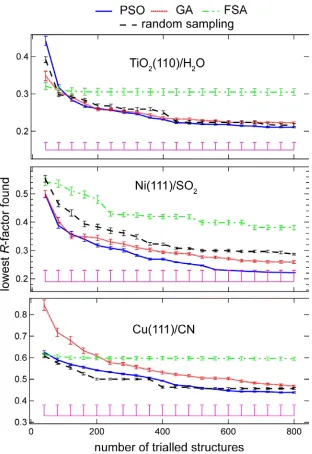
Of the other two fitting algorithms, the PSO achieves the lowest R-factors for all the model systems, although its advantage over GA is marginal for TiO2(110)/H2O
and modest for the Cu(111)/CN system. PSO outperforms the random sampling
for all three model systems, while GA marginally fails to achieve this for the
Cu(111)/CN system. The Cu(111)/CN system was identified as the most complex
problem to solve, with the largest number of fitting parameters and an expectation
that even the best R-factor minimum will be shallow in the variable hyperspace; as such, the limitation of 20 iterations (800 trialled models) used here is unlikely to
be sufficient to find the bottom of the global minimum. The fact that both the PSO
and GA implementations show a slight downwards gradient at the end of the test
supports this view. Indeed, in our previous application of the PSO algorithm to aid
the solution of PhD structure determination [14,15,16] we have always used more
than 20 iterations to achieve more reliable convergence, but this smaller number of
iterations appears sufficient to show the general trends of the different methods.
While the results of Fig. 4 provide information as to which algorithm finds the
lowest R-factor in the smallest amount of computational time, a further important question is whether the structures corresponding to the lowest R-factor values are the correct structure. Have the searches identified the region of variable parameter
hyperspace corresponding to the true global minimum, and have they located the
bottom of this global minimum? The first of these two questions is the most
important one. A steepest gradient search will locate the true R-factor far more quickly that any of these algorithms if it is started within the global minimum, and
in our previous applications of the PSO algorithm [14,15,16] we have used such a
gradient search to refine structures identified using PSO. However, if a gradient
escape this minimum. The important question is therefore whether the global
search algorithms have located the correct region of parameter space
corresponding to the global minimum for each system, or have only converged on
local minima.
In addition to the R-factor values obtained during the progress of the different search algorithms, Fig. 4 also shows, as a horizontal (pink) line, the value of the R -factors obtained in the original structure determination of each of the model
systems. It is notable that for all three systems this value is lower than that
achieved in any of the search methods, providing further support for the idea that
the original analyses (that included structural optimisations using a gradient search
algorithm) did identify the true structures. We may therefore ask how similar are
the best structures found by the different global search algorithms (after 20
iterations) to these ‘true’ structures. In performing structure determinations using
the PhD technique, the ultimate precision of the method can be determined by
calculating the variance of the (minimum) value of the R-factor found for the best-fit structure, var(Rmin). This variance depends on the size of the data set used in the analysis and the value of the lowest R-factor [25]. Any structure that leads to a value of the R-factor less than (Rmin+var(Rmin)) is regarded as falling within the limits of precision, and therefore an acceptable solution, and simple calculations
allow one to define error estimates for each of the structural parameters.
To determine how similar the best structures found by the global search algorithms
are to the ‘true’ structures, we can therefore use the difference between the values
of the best-found R-factor, and the R-factor for the ‘true’ structure. This is most
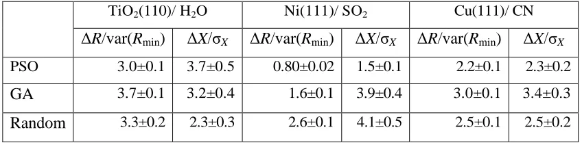
appropriately defined relative to the variance in R, by the ratio ΔR/var(Rmin). Similarly, we can also compare the size of the deviations of the structural
parameters from the ‘true’ structures with the estimated errors in these parameters,
by the ratio ΔX/σX. This latter value provides a more direct indication of whether
the global search algorithms have located the region of parameter space
corresponding to the global minimum (which we infer, from the arguments above,
are listed in Table 1. Note that, even though the implementations of the PSO ands
GA algorithms are fairly basic, they both appear to converge in the area of the
‘true’ structure with a comparable level of accuracy. Both algorithms could
probably be further optimised to solve these three specific problems more fully,
but these two simple implementations provide acceptable results.
As shown in Figure 4, and quantified in Table 1, for the Ni(111)/SO2 structure
PSO locates a model within the variance (ΔR/var(Rmin)<1) of the ‘correct’ structure, although the fact that ΔX/σX>1 suggests that there may be some
parameter coupling in the simulations, such that an increase in R due to a change in one parameter value may be compensated by a reduction due to a change in
another. For this system GA also finds an R-factor value only slightly larger than the variance of the true structure, though the actual parameter values show
significantly larger variations. Most of the other values of Table 1 reinforce the
information provided by visual inspection of Fig. 4. For the Cu(111)/CN system
PSO yields a model significantly closer to the ‘correct’ structure than GA,
although only marginally better than the random sampling. For the TiO2/H2O
system the three methods yield surprisingly similar results, although it is the
random sampling that shows the lowest deviation from the ‘true’ structure in terms
of the structural parameter values.
4. Conclusions
Three stochastic global search algorithms have been tested for application in
energy-scanned photoelectron diffraction. In particular, we have described the
implementation and results of a particle swarm optimisation algorithm, and
compared its performance with that of a genetic algorithm, fast simulated
annealing, and random sampling. In all cases the objective was to locate the
approximate structure solution in an unbiased fashion. The use of only 20
iterations appears to be sufficient to provide valuable information on the relative
merits of at least three of these different approaches, but also almost certainly
Ni(111)/SO2) yielded a solution within the variance of the ‘true’ structure.In these
tests no attempt was made to achieve final structural optimisation. When using the
PSO in full structure determinations (e.g. [14,15,16]) a significantly larger number
of iterations have been used. Moreover, once the global search has converged, a
gradient search (specifically, in the structure determinations mentioned above, a
Levenberg-Marquardt algorithm [26]) is able to locate the bottom of that particular
minimum far more quickly than any global search algorithm. The important
requirement for the global search is thus only that it locates the R-factor well that contains the global minimum
Both the PSO and GA methods have been found to be applicable to PhD surface
structure determination, although the PSO proved better in some cases and worse
in none. It is possible that the slightly inferior performance of the GA relative to
PSO stems from the discrete nature of this approach. The GA is specifically
designed for use in a discrete variable space, hopping between the different values
that are present in the population, whereas PSO is designed for a continuous
search space, crawling between the values that have already been calculated. The
other significant advantage of PSO is its use of memory. The GA, apart from the
elitism, does not actively utilise the shared knowledge of the population, whereas
in PSO the best-found structure for each individual of the population is always
remembered, as is the best-found structure that each member of the population has
been informed of.
One surprising result of our tests is that for two of the systems (TiO2(110)/H2O
and Cu(111)/CN) the PSO and the GA achieved results that were only marginally
better than, or even slightly worse than, the random sampling. The results of our
tests of the FSA approach were particularly disappointing, with this method failing
to make substantial progress in the structural search in any of the three systems
tested. Possible reasons for this are discussed in the previous section.
Of course, it is dangerous to draw very general conclusions about the relative
implementations for just three model systems. All three techniques use preset
parameters, the values of which can have a significant effect on their efficacy.
Specifically, in the genetic algorithm, there are two parameters that define the rate
of mutation, and in the PSO there are the three parameters (cp, cl and cg) that
weight the influence of the three components of Eqn. 6. Optimisation of these
parameters was not pursued extensively in this study due to limited computational
resources. A different set of inputted parameters could make the GA at least as
effective as the PSO implementation; however, an important conclusion is that this
new PSO approach is at least comparable in efficacy to the better known and more
widely applied genetic algorithm.
In summary, our main conclusion is that at least two of these algorithms (GA and
PSO), even in these basic implementations, can be used with good effect to search
the variable hyperspace in PhD, and thus contribute in a useful way to the
structural solution. A more surprising result is that an automated random sampling
may also be valuable.
Acknowledgement
The authors acknowledge the partial support of the Engineering and Physical
Sciences Research Council (UK) for this work. The computing facilities were
provided by the Centre for Scientific Computing of the University of Warwick
with support from the Science Research Investment Fund. The authors would also
like to acknowledge Dr F. Filsinger of the Fritz-Haber-Institut, Berlin for
suggesting genetic algorithms for this application, Dr. W. Unterberger, also of the
Fritz-Haber-Institut, for providing the CN on Cu(111) data, and Dr. F. Allegretti of
Table 1: Average difference between the previously-determined ‘correct’
structure of each system, and the structures found using the two algorithms
(PSO and GA) and random sampling expressed as normalised differences in
the R-factor or the coordinates, as described more fully in the text.
TiO2(110)/ H2O Ni(111)/ SO2 Cu(111)/ CN
ΔR/var(Rmin) ΔX/σX ΔR/var(Rmin) ΔX/σX ΔR/var(Rmin) ΔX/σX
PSO 3.0±0.1 3.7±0.5 0.80±0.02 1.5±0.1 2.2±0.1 2.3±0.2
GA 3.7±0.1 3.2±0.4 1.6±0.1 3.9±0.4 3.0±0.1 3.4±0.3
[image:19.596.93.517.174.280.2]Figure Captions
Figure 1: The blue line shows a hypothetical variation of the R-factor with one variable parameter in which there are multiple mimina. Superimposed is a
comparison of Gaussian (black dashed) and Lorentzian (red solid) distribution
sampling. In this example, in which the current model is centred on the local
minimum A, the Lorentzian has a longer “tail” and will thus lead to an
increased probability that subsequent iterations may allow the search
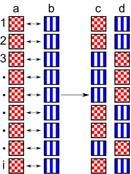
Figure 2: Schematic representation of crossover in genetic algorithms. The two
chosen “parents” (a and b) produce two children (c and d). Whether child c or child d gains each coordinate, 1 to I, from parent a or b is chosen randomly.
Here the coordinates of a are represented by a chequered red box, and b by blue vertical lines. Each coordinate of the child has an equal chance of receiving the
coordinate from either parent, and we end up with an intermixing of the two
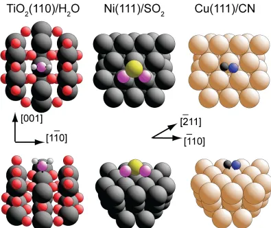
Figure 3: Schematic diagrams (in plan and perspective views) of the structures
previously determined by PhD of TiO2(110)/H2O, Ni(111)/SO2, and
Cu(111)/CN. Substrate metal atoms are shown as the largest spheres, while the
radii chosen to represent other atoms increase with increasing atomic number in
individual structures from H to C, N, O and S. Note that in the TiO2(110)/H2O
structure the O atom of the water is shown in a different colour (shading) from
Figure 4: Comparison of the dependence of the lowest R-factor found on the number of trialled structural models for the three fitting algorithms and a
random sampling of the variable hyperspace, for each of the substrate/adsorbate
data sets investigated. Each value represents the average of 10 different repeats
of the calculations with different (random) starting structures. The R-factor achieved in the original structure determinations [21,23,24] is shown by the
horizontal (pink) lines at the bottom of each panel, with their variances shown as
23
References
[1] D.P. Woodruff, Surf. Sci. Rep., 62 (2007) 1.
[2] J.B. Pendry, J. Phys. C: Solid State Physics, 13 (1980) 937.
[3] M.L. Viana, R. Díez Muiño, E.A. Soares, M.A. Van Hove, V.E. de
Carvalho, J. Phys.: Condens. Mat., 19 (2007) 446002.
[4] A. Pancotti, P.A.P. Nascente, A. de Siervo, R. Landers, M.F.
Carazzolle, D.A. Tallarico, G.G. Kleiman, Top. Catal, 54 (2011) 70.
[5] A. Pancotti, N. Barrett, L.F. Zagonel, G.M. Vanacore, J. Appl. Phys.,
106 (2009) 034104.
[6] A. Pancotti, A. de Siervo, M.F. Carazzolle, R. Landers, G.G. Kleiman,
Top. Catal., 54 (2011) 90.
[7] R. Döll, M.A. Van Hove, Surf. Sci., 355 (1996) L393.
[8] V.B. Nascimento, V.E. de Carvalho, C.M.C. de Castilho, E.A. Soares,
C. Bittencourt, D.P. Woodruff, Surf. Rev. Lett., 6 (1999) 651
[9] V.B. Nascimento, V.E. de Carvalho, C.M.C. de Castilho, B.V. Costa,
E.A. Soares, Surf. Sci., 487 (2001) 15
[10] M. Kottcke, K. Heinz, Surf. Sci., 376 (1997) 352.
[11] Z. Zhao, J.C. Meza, M.A. Van Hove, J. Phys.: Condens. Matter, 18
(2006) 8693.
[12] M. Clerc, Particle Swarm Optimisation, ISTE Ltd, London 2006
[13] J. Kennedy, R. Eberhart, Proc. IEEE Internat. Conf. Neural Networks,
4 (1995) 1942
[14] M.K. Bradley, D.A. Duncan, J. Robinson, D.P. Woodruff, Phys.
Chem. Chem. Phys., 13 (2011) 7975.
[15] D.A. Duncan, W. Unterberger, D. Kreikemeyer-Lorenzo, D.P.
Woodruff, J. Chem. Phys., 135 (2011) 014704.
[16] D.C. Jackson, D.A. Duncan, W. Unterberger, T.J. Lerotholi, D.
Kreikemeyer-Lorenzo, M.K. Bradley, D.P. Woodruff, J.Phys. Chem. C,
24
[17] V. Fritzsche, Surf. Sci., 265 (1992) 187.
[18] V. Fritzsche, J. Phys.: Condens. Matter, 2 (1990) 1413.
[19] V. Fritzsche, Surf. Sci., 213 (1989) 648.
[20] V. Fritzsche, J.B. Pendry, Phys. Rev. B, 48 (1993) 9054.
[21] M.J. Knight, F. Allegretti, E.A. Kröger, K.A. Hogan, D.I. Sayago, T.J.
Lerotholi, W. Unterberger, D.P. Woodruff, Surf. Sci., 603 (2009) 2062
[22] M. Affenzeller, S. Winkler, S. Wagner and A. Beham, Genetic
Algorithms and Genetic Programming, CRC Press, Boca Rotan, Florida 2009
[23] F. Allegretti, S. O'Brien, M. Polcik, D.I. Sayago, D.P. Woodruff, Surf.
Sci., 600 (2006) 1487.
[24] M. Polcik, M. Kittel, J.T. Hoeft, R. Terborg, R.L. Toomes, D.P.
Woodruff, Surf. Sci., 563 (2004) 159
[25] N.A. Booth, R. Davis, R. Toomes, D.P. Woodruff, C. Hirschmugl,
K.M. Schindler, O. Schaff, V. Fernandez, A. Theobald, Ph. Hofmann, R.
Lindsay, T. Gießel, P. Baumgärtel, A.M. Bradshaw, Surf. Sci., 387 (1997)
152
[26] H. William, S. Teukolsky, W. Vetterling, F. Flannery, Numerical