Original citation:
Petrella, Ivan, Rossi, Raffaele and Santoro, Emiliano. (2014) Discretion vs. timeless
perspective under model-consistent stabilization objectives. Economics Letters, 122 (1). pp. 84-88.
Permanent WRAP URL:
http://wrap.warwick.ac.uk/88222
Copyright and reuse:
The Warwick Research Archive Portal (WRAP) makes this work by researchers of the University of Warwick available open access under the following conditions. Copyright © and all moral rights to the version of the paper presented here belong to the individual author(s) and/or other copyright owners. To the extent reasonable and practicable the material made available in WRAP has been checked for eligibility before being made available.
Copies of full items can be used for personal research or study, educational, or not-for-profit purposes without prior permission or charge. Provided that the authors, title and full bibliographic details are credited, a hyperlink and/or URL is given for the original metadata page and the content is not changed in any way.
Publisher’s statement:
© 2014, Elsevier. Licensed under the Creative Commons Attribution-NonCommercial-NoDerivatives 4.0 International http://creativecommons.org/licenses/by-nc-nd/4.0/
A note on versions:
The version presented here may differ from the published version or, version of record, if you wish to cite this item you are advised to consult the publisher’s version. Please see the ‘permanent WRAP url’ above for details on accessing the published version and note that access may require a subscription.
1
Introduction
Woodford (1999, 2003) has in‡uentially argued that monetary policy should be conducted from a timeless perspective, a policy that helps overcoming both the traditional in‡ation bias (Barro and Gordon, 1983) and the stabilization bias (Svensson, 1997 and Clarida et al., 1999). Despite the direct advantages of such a commitment technology, Sauer (2010a, 2010b) reports situations in which, depending on the initial conditions of the economy, timeless perspective may be inferior to discretion. Dennis (2010) details similar …ndings, proposing a conditional loss function as a valid metric to assess the relative performance of alternative policy regimes.1 These results hinge on the role of elements that reduce the slope of the New Keynesian Phillips curve (NKPC hereafter), such as nominal price rigidities, …rm-speci…c labor/capital, and Kimball (1995) aggregation, as well as on the policy maker’s preference for output stabilization. The common trait of these factors is to raise the conditional volatility of the auxiliary state variables that track the value of commitments under timeless perspective, so that discretion becomes the superior policy. This paper shows that comparing the performance of discretionary policy-making rel-ative to that of timeless perspective should necessarily rest on a welfare-theoretic function that is consistent with the underlying structure of the model economy. In other words, to avoid a spurious welfare ranking the policy maker’s objective function should accurately represent households’preferences, as well as potential sources of real and nominal rigid-ity. The existing studies have not taken such a standpoint, as their analysis has typically dealt with linear-quadratic problems where the Central Bank’s preferences are de-linked from the deep parameters of the model. This point turns out to be of crucial importance for reporting situations in which discretion dominates timeless perspective. To show this, we examine the baseline New Keynesian model that has been used by Dennis (2010) and Sauer (2010a, 2010b). Along with considering a standard microfoundation for this model economy, we replace their policy makers’ objective functions with a welfare criterion obtained as a second-order approximation of households’utility (Rotemberg and Wood-ford, 1998). Within this setting most of the factors that a¤ect the slope of the NKPC also in‡uence the policy maker’s preferences for alternative stabilization objectives. For instance, increasing the degree of nominal rigidity has the joint e¤ect of reducing the slope of the NKPC and increasing the relative importance of in‡ation stabilization in the ‘model-consistent’welfare criterion. The second e¤ect reduces the short run cost of being tough on in‡ation already in the initial period, so that timeless perspective is favored over discretion.
In light of our analysis, discretion should have higher chances of dominating timeless perspective if we can envisage structural elements that lower the slope of the NKPC while not increasing the relative weight attached to in‡ation stabilization (or vice versa). To this end, Petrella and Santoro (2011) have shown that allowing for input materials in the production technology lowers the slope of the NKPC without a¤ecting the Central Bank’s objective function. Input materials also correspond to the largest determinant of the total cost of production in various industries2 and, as such, they exert strong in‡uence on the
1Since timeless perspective involves the existence of auxiliary state variables that discretion does
not feature, comparing their relative performance requires an appropriate welfare metric. Instead of assigning initial values to the auxiliary state variables or using unconditional losses, Dennis (2010) employs a measure of conditional loss that integrates out the auxiliary state variables, conditional upon the predetermined state variables.
2Dale Jorgenson’s data on input expenditures by US industries show that materials (including energy)
slope of the aggregate supply schedule (Basu, 1995). We show that input materials enhance the performance of discretion relative to timeless perspective. However, even strong degrees of strategic complementarity stemming from input-output interactions are ine¤ective at making discretion the superior policy when welfare is evaluated through a model-consistent metric.
The remainder of the paper is laid out as follows: Section 2 presents the model; Section 3 compares the relative performance of discretionary and timeless perspective policy-making: we check the robustness of our results over a wide range of values for the deep parameters of the model economy, as well as alternative institutional settings for the conduct of monetary policy; Section 4 concludes.
2
The Model
This section presents the equations to be employed in the normative analysis. These are derived from a dynamic general equilibrium New Keynesian model that accommodates the presence of input materials in the production technology.3 Firms operate within a monopolistically competitive setting and set prices according to a Calvo (1983) scheme. As in Basu (1995) the production technology embodies both labor and intermediate goods, so that the gross product of each …rm is both consumed and used in the production of all other goods in the economy. It is important to recognize that setting the income share of input materials to zero renders the model economy identical to the standard New Keynesian setting popularized by, e.g., Woodford (2003).
Households derive income from working in …rms, investing in bonds, and from the stream of pro…ts generated by …rms in the economy. The government serves two purposes in the economy. First, it delegates monetary policy to an independent Central Bank. The second task of the government consists of taxing households and providing subsidies to …rms to eliminate distortions arising from monopolistic competition in the goods market.4 This task is pursued via lump-sum taxes that maintain a balanced …scal budget.
2.1
Solution and Calibration
Prior to step into our normative analysis, we log-linearize structural equations and re-source constraints around the non-stochastic steady state and then take the deviation from their counterparts in the e¢ cient equilibrium. The di¤erence between the loga-rithm of a generic variable Xt under sticky prices and its counterpart in the e¢ cient
equilibrium, Xt, is denoted by xt.5 The rate of in‡ation, t, evolves in accordance with
the following NKPC:
t= Et t+1+ ( + ) (1 )ct+ t; (1)
where ct represents the consumption gap, denotes the discount factor, denotes
the inverse of the intertemporal elasticity of substitution, denotes the inverse of the
3A detailed description of the framework is available in the Technical Appendix.
4For the sake of making a correct welfare ranking between discretion and timeless perspective within
our linear-quadratic framework, steady state e¢ ciency is mandatory (Woodford, 2003). Otherwise, in the presence of no subsidy the steady state would be distorted, leading to a spurious welfare analysis.
Frisch elasticity of labor supply, denotes the income share of input materials, de-notes the probability that …rms are not able to adjust their price in each period,
(1 ) (1 ) 1 and t (" 1)
1
ln ("t="). Therefore, a negative shock to the
degree of competition (i.e., a lower "t) translates into a positive cost-shifter. We impose ln ("t=") = ln ("t 1=") + t, where 2(0;1)and t is assumedi:i:d: with zero mean and
unit variance.
The income share of input materials is a key determinant of the slope of the supply schedule.6 In a hypothetical situation with intermediate goods as the only production input (i.e., = 1) current in‡ation would be insulated from movements in the real wage, so that strategic complementarities in the market for intermediate goods would render the NKPC completely ‡at.
To evaluate the in‡uence of the structural coe¢ cients on the performance of discre-tion relative to timeless perspective, each of them will be varied while leaving the other parameters at the following values: = 0:9913, = 1, = 0:2, = 0:75,"= 6, = 0:2.7 Finally, we set = 0 in the baseline parameterization, so as to collapse the model to the baseline New Keynesian setting and enhance the comparison with previous studies in the same strand of the literature.
3
Monetary Policy
The next step consists of taking a second-order Taylor approximation to the representa-tive household’s lifetime utility (see Rotemberg and Woodford, 1998).8 In line with the analysis of Petrella and Santoro (2011), the following intertemporal social loss function is obtained:
W0
UCC
2 E0
1
X
t=0
t
( + )c2t + 2t +t.i.p.+O k k3 ; (2)
whereC denotes the steady state level of consumption,UC is the (steady state) marginal
utility with respect toCt, t.i.p. collects the terms independent of policy stabilization and
O k k3 summarizes all terms of third order or higher. A peculiarity of (2) is that the preference for in‡ation stabilization, " 1, does not depend on . This is an inherent property of the model-consistent welfare criterion, which weighs in‡ation variability with consumption gap variability, rather than output gap variability (Petrella and Santoro, 2011 and Petrella et al., 2013).
Under discretionary policy-making the Central Bank faces a sequence of static op-timization problems, disregarding the impact of her policies on in‡ation expectations.
6We should stress that the presence of a subsidy that neutralizes the steady state ine¢ ciency
emanat-ing from monopolistic competition implies that the consumption gap equals the labor gap (i.e.,ct=lt)
under any value of the income share of input materials, and not only for = 0. In this respect, the slope
of our NKPC is coherent with the derivations of Bergin and Feenstra (2000), Woodford (2003, Eq. 2.13, Ch. 3) and Huang and Liu (2004).
7This value for the autoregressive process of the cost-shifter is chosen in line with Dennis (2010).
8We assume that shocks that hit the economy are not big enough to lead to paths of the endogenous
Minimizing (2) subject to (1) – taking in‡ation expectations Et t+1 as given – results into:
t=
1
"(1 )ct: (3)
Should the policy maker be able to credibly commit herself to some future policy path, she can minimize (2) by internalizing the impact of her actions on expectations. The optimality conditions in this case involve (3) for t= 0, together with
t=
1
"(1 )(ct ct 1); t= 1;2; ::: (4)
Equation (4) accounts for the possibility to spread the e¤ects of shocks over several periods. Yet, commitment is time inconsistent in two ways: …rst, the policy maker can switch from (4) to (3) in any period after t = 0, exploiting given in‡ation expectations. Second, as argued by McCallum (2003) each period the policy maker faces an incentive to depart from its previous optimized plan, so that ‘strategic incoherence’characterizes the policy path.
Woodford (1999, 2003) has originally proposed a ‘timeless perspective’ approach to overcome the second form of time inconsistency. This involves ignoring the conditions that prevail at the regime’s inception, thus imagining that the commitment to apply the rules deriving from the optimization problem had been made in the distant past. Under timeless perspective (4) applies from t= 0 onwards.
3.1
Policy Evaluation
The short run costs from adhering to the timeless perspective policy are generally ampli-…ed in the presence of elements that reduce the slope of the NKPC, or when the monetary authority poses increasing emphasis on consumption stabilization. Under these circum-stances the Central Bank must generate greater volatility in the real marginal costs, so as to stabilize in‡ation. According to the existing literature, to the extent that real marginal costs are correlated with the Central Bank’s other policy objectives, higher volatility in real marginal costs raises the volatility of the commitments that characterize timeless perspective, so that discretion may become the superior policy.
In the present setting timeless perspective policy-making involves one auxiliary state variable,ct 1. Rather than assigning initial values or using unconditional losses, we follow
Dennis (2010), who has formulated a measure of conditional loss that integrates out the auxiliary state variables conditional upon the known predetermined state variables. This strategy is consistent with the conditioning assumptions that describe the optimization problems and provides a consistent treatment of the initial conditions in the equilibria under alternative regimes. Finally, to assess the relative loss induced by alternative policies we follow Sauer (2010a, 2010b) and compute
RL= W
tp
where Wd denotes the conditional loss under discretion and
Wtp is the conditional loss
under timeless perspective. RL measures the percentage gain from implementing dis-cretion over timeless perspective. In each panel of Figure 1 we report both the relative loss under the microfounded welfare criterion, as well as under a loss function with …xed preferences similar to that considered by Dennis (2010) and Sauer (2010a, 2010b).9
Insert Figure 1 here
We …rst focus on the role of price stickiness, whose importance has been very much emphasized due to its e¤ect on the slope of the NKPC. Our simulation shows that the relative loss under …xed preferences for the policy maker increases monotonically, while the one consistent with (2) displays a U-shaped pattern over the domain of . Most importantly, timeless perspective is dominated by discretion only at implausibly high values of and when the policy maker considers an ad hoc welfare criterion. Otherwise, this is never the case when the relative loss is evaluated through a model-consistent metric. To explain this result we need to consider that increasing has three main e¤ects: …rst, …rms attach greater importance to future pro…ts, as they have fewer chances to adjust their prices. This incentive favors timeless perspective over discretion, as the former optimally incorporates forward-looking expectations. Second, more rigid prices reduce the pass-through from the real marginal cost to the rate of in‡ation, so that timeless perspective entails higher costs of being tough on in‡ation already in the initial period. The third e¤ect –which has not been explored by the literature available to date –is that increasing lowers the relative weight attached to consumption gap variability in (2), so that the short run cost of being tough on in‡ation in the initial period decreases. The importance of the last e¤ect may be inferred from the wedge between the two relative losses in the …rst panel of Figure 1. Under thead hoc function the weight on consumption stabilization does not depend on , so that the second e¤ect tends to prevail over the …rst one (though at extremely high values of ). By contrast, with the microfounded welfare function the third e¤ect comes into play and, adding up to the …rst one, it makes timeless perspective prevail over discretion throughout the entire range of values of . This general principle also applies to the parameters governing households’relative risk aversion and the elasticity of labor supply. As a matter of fact, alternative values of these coe¢ cients never induce a better performance of discretion. Yet, increasing and/or improves the performance of discretion relative to timeless perspective under a microfounded welfare criterion, while the opposite holds true under the ad hoc loss function. In the …rst case, the increase in the weight attached to consumption stabilization overcomes the positive e¤ect on the slope of the NKPC, while in the second case the slope of the NKPC increases in both and , so that discretion is penalized. It should also be noted that, consistent with Sauer (2010a), discretion loses relative to timeless perspective if increases. This is because the so-called ‘expectations channel’becomes increasingly important, overcoming the rise in the short run costs associated with timeless perspective, which arise from exerting a negative e¤ect on the slope of the NKPC. This e¤ect is magni…ed when (2) is accounted for, as increasing also translates into increasing the relative weight attached to in‡ation stabilization, through .
We also examine the role of parameters that do not have direct in‡uence on the slope of the NKPC. In this respect, we note that the relative loss decreases with : Sauer
9Speci…cally, we follow Dennis (2010) and set the preference for consumption stabilization to 0:5,
(2010a) suggests that timeless perspective has to be preferred when shocks dissipate more slowly and exert greater in‡uence on the future, though he also shows that appropriate combinations of other parameters may even revert the in‡uence of on RL. It is also worth noting that RL is insulated from movements in " under the ad hoc welfare func-tion,10 while it decreases when we consider the microfounded metric. This is because higher competition necessarily increases the weight attached to in‡ation stabilization in (2), thus favoring timeless perspective over discretion.
The last panel of Figure 1 evaluates the e¤ect of increasing on the relative perfor-mance of timeless perspective. When input materials are part of the production technol-ogy and prices are sticky, …rms face constant costs for their inputs, so that the sensitivity of the real marginal cost to variations in aggregate demand are rather small. In turn, …rm-level incentives to cut prices and increase output are reduced (Basu, 1995). There-fore, input-output interactions have the potential to turn small price-setting frictions into considerable degrees of real rigidity. In addition, has no impact on (2). Altogether, these factors turn out to be important in that they induce the relative loss to increase over a range of plausible values of the income share of input materials.11 However, strategic complementarities stemming from input-output interactions never prevent timeless per-spective from dominating discretion, even when the policy maker has a strong preference for consumption stabilization.12
3.2
Delegation
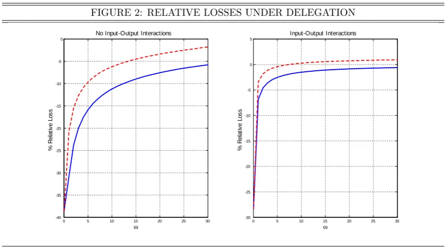
The analysis so far has stressed the importance of measuring social welfare through a model-consistent metric when comparing alternative policies. However, it could be argued that such a metric is not known with certainty and/or the government may delegate monetary policy to an independent Central Banker whose preferences for alternative stabilization objectives di¤er from those of the public as whole (see, e.g., Rogo¤, 1985). Under these circumstances we could envisage a de-linking between the deep parameters a¤ecting the slope of the NKPC and the preferences of the policy maker. The aim of this section is to understand whether our key insight is robust to this critique. To this end, we retrieve the optimal rules under a welfare criterion where the weight on consumption stabilization –which will be denoted by! –is allowed to vary, while the one on in‡ation stabilization is normalized to one. In turn, welfare is evaluated both under the model-consistent metric (2), as well as under the loss function of the delegated Central Banker. The results of this exercise are graphed in Figure 2.
Insert Figure 2 here
It turns out that under the baseline calibration timeless perspective dominates dis-cretion even when the Central Banker faces an ad hoc criterion and welfare is evaluated accordingly (i.e., when the policy maker evaluates the loss of social welfare in accordance
10This is because under thead hoc welfare function"only a¤ects the elasticity of
tto the stochastic
cost-shifter. Therefore, varying" results into the same e¤ect on both Wtp and Wd, so that RL is not
in‡uenced by changes in the degree of monopolistic competition.
11Under the ad hoc criterion RL increases monotonically. Otherwise, the relative loss displays an
increasing path only for greater than about0:3.
12To appreciate a better performance of discretion relative to timeless perspective under the ad hoc
welfare criterion we would need to couple a plausible degree of input-output interactions ( 0:6) with
with her preferences, while disregarding those of the public). Introducing input materials ( = 0:6) allows discretion to outperform timeless perspective under a strong preference for consumption stabilization (i.e.,!greater than about7), but only when welfare is com-puted through the ad hoc function. Otherwise, this is never the case when the optimal policies are derived from the loss function of the delegated Central Banker and welfare is evaluated through the model-consistent metric.
4
Conclusions
Recent contributions have reported situations in which the short run costs associated with timeless perspective policy-making dominate the long run gains with respect to discretion, so that the latter may become the superior policy (Dennis, 2010; Sauer, 2010a, 2010b).
Figures
FIGURE 1: RELATIVE LOSSES
0.6 0.7 0.8 0.9
-40 -20 0 % R elat iv e Los s
θ
0 1 2 3-30 -20 -10
ν
1 2 3 4 5
-40 -20 0 % R elat iv e Los s
σ
0 0.2 0.4 0.6
-40 -20 0 % R elat iv e Los s
α
0 0.2 0.4 0.6 0.8
-100 -50 0
ρ
% R elat iv e Los s5 10 15 20
-30 -20 -10
ε
0.9 0.92 0.94 0.96 0.98 -40
-20 0
β
Notes. Each panel of the …gure portrays the relative loss (RL) conditional on di¤erent values of
FIGURE 2: RELATIVE LOSSES UNDER DELEGATION
0 5 10 15 20 25 30 -40
-35 -30 -25 -20 -15 -10 -5 0
%
Rel
at
iv
e
Los
s
No Input-Output Interactions
ω 0 5 10 15 20 25 30
-30 -25 -20 -15 -10 -5 0 5
Input-Output Interactions
ω
%
Rel
at
iv
e
Los
s
Notes. Figure 2 portrays the relative loss (RL) conditional on di¤erent values of the delegated
Central Banker’s preference for consumption stabilization (the weight attached to in‡ation stabilization is set to one): the dashed line represents the relative loss for the delegated Central Banker, while the continuous line represents the relative loss from the perspective of the public. In the LHS panel all other parameters are set in line with the baseline parameterization described in Section 2.1, while in the RHS
Technical Appendix: The Model
We embed an input-output production structure into an otherwise standard dynamic gen-eral equilibrium New Keynesian model. Firms operate within a monopolistically compet-itive setting. Their production technology embodies both labor and intermediate goods, so that the gross product of each …rm in the economy is both consumed and used in the production of all other goods in the economy.
Consumers
Households derive income from working in …rms, investing in bonds, and from the stream of pro…ts generated by …rms in the economy. They have preferences de…ned over a composite of goods (Ct) and labor (Lt). They maximize the expected present discounted
value of their utility:
E0
1
X
t=0
t C
1
t
1 %
L1+t
1 + ; % >0 (6)
where is the discount factor, is the inverse of the intertemporal elasticity of substi-tution, is the inverse of the Frisch elasticity of labor supply.
The following sequence of (nominal) budget constraints applies:
PtCt+Bt =Rt 1Bt 1+PtWtLt Tt+ t; (7)
where Pt is the price of the composite good, Bt denotes a one-period risk-free nominal
bond remunerated at the gross risk-free rate Rt 1 + it, Wt is the real wage rate, Tt
is a lump-sum tax paid to the government and t is the aggregate nominal ‡ow of …rm
dividends.
Producers
The production side of the economy consists of one sector producing a continuum of di¤erentiated goods i 2 [0;1]. We assume that the consumption composite takes the form of a Dixit-Stiglitz aggregator:
Ct = Z 1
0
(Cit)
"t 1
"t di "t "t 1
; (8)
where "t denotes the time-varying elasticity of substitution between di¤erentiated goods
in the consumption composite. It is possible to show that a generic …rm i faces the following demand schedule:
Cit =
Pit
Pt "t
Ct; (9)
As in Basu (1995), Bergin and Feenstra (2000) and Moro (2009) we assume a Cobb-Douglas production technology for a generic …rmi:13
Yit =ZtMitL
1
it ; (10)
whereZt is a productivity shifter,Lit denotes the number of hours worked in the ith …rm
and Mit denotes the amount of material inputs employed by …rm i. Material inputs are
combined according to a CES aggregator:
Mit = Z 1
0
(Mkit)
("t 1)="t
dk
"t=("t 1)
; (11)
whereMkit is the intermediate input produced by …rmk and employed in the production
process of …rm i. This speci…cation implies the following demand function for the kth
intermediate good:
Mkit=
Pkt
Pt "t
Mit: (12)
The gross product of the ith …rm may be sold on the market for …nal consumption goods
or used as an intermediate good by all …rms in the economy, so that Yit =Cit+Mit.
Firms are assumed to adjust their price with probability 1 in each period. When they are able to do so, they set the price that maximizes expected pro…ts:
max
Pit Et
1
X
n=0
( )n t+n[(1 + )Pit M Cit+n]
Yit+n
Pt
(13)
where tis the stochastic discount factor consistent with households’maximizing
behav-ior, is a steady state subsidy to producers14 andM C
itdenotes …rm’sinominal marginal
cost of production. In every period each …rm solves a cost minimization problem to meet demand at its stated price, so that:
M Cit =
PtWtLit
(1 )Yit
= PitMit
Yit
: (14)
The Government and the Monetary Authority
The government serves two purposes in the economy. First, it delegates monetary policy to an independent Central Bank. The second task of the government consists of taxing
13The key insights reported in the remainder of this paper are valid under more general production
technologies, such as the CES speci…cation of Dotsey and King (2006).
14The subsidy will be set so as to neutralize the monopolistic competition ine¢ ciency in the steady
households and providing subsidies to …rms to eliminate distortions arising from monop-olistic competition in the markets for both classes of consumption goods. This task is pursued via lump-sum taxes that maintain a balanced …scal budget.
References
Barro, R. J., and D. B. Gordon (1983): “A Positive Theory of Monetary Policy in
a Natural Rate Model,”Journal of Political Economy, 91(4), 589–610.
Basu, S.(1995): “Intermediate Goods and Business Cycles: Implications for
Productiv-ity and Welfare,”American Economic Review, 85(3), 512–31.
Bergin, P. R., and R. C. Feenstra(2000): “Staggered price setting, translog
prefer-ences, and endogenous persistence,”Journal of Monetary Economics, 45(3), 657–680.
Calvo, G. A.(1983): “Staggered prices in a utility-maximizing framework,”Journal of
Monetary Economics, 12(3), 383–398.
Dennis, R.(2010): “When is discretion superior to timeless perspective policymaking?,”
Journal of Monetary Economics, 57(3), 266–277.
Dotsey, M., and R. G. King(2006): “Pricing, Production, and Persistence,”Journal
of the European Economic Association, 4(5), 893–928.
Huang, K. X., and Z. Liu (2004): “Input Output Structure And Nominal Rigidity:
The Persistence Problem Revisited,”Macroeconomic Dynamics, 8(02), 188–206.
Kimball, M. S. (1995): “The Quantitative Analytics of the Basic Neomonetarist
Model,”Journal of Money, Credit and Banking, 27(4), 1241–77.
McCallum, B. T. (2003): “Comment on Athey, Atkeson, and Kehoe, ’The Optimal
Degree of Monetary Policy Discretion’,” Discussion, Second International Research Forum on Monetary Policy, Washington, DC, November 14-15.
Moro, A.(2009): “Input-Output Structure and New Keynesian Phillips Curve,”Rivista
di Politica Economica, 99(2), 145–166.
Petrella, I., R. Rossi, and E. Santoro (2013): “Monetary Policy with Sectoral
Trade-o¤s,” mimeo, University of Copenhagen.
Petrella, I.,and E. Santoro(2011): “Input-Output Interactions and Optimal
Mon-etary Policy,”Journal of Economic Dynamics and Control, 35, 1817–1830.
Rogoff, K.(1985): “The Optimal Degree of Commitment to an Intermediate Monetary
Target,”The Quarterly Journal of Economics, 100(4), 1169–89.
Rotemberg, J. J., andM. Woodford (1998): “An Optimization-Based Econometric
Framework for the Evaluation of Monetary Policy: Expanded Version,” NBER Tech-nical Working Papers 0233, National Bureau of Economic Research, Inc.
Sauer, S.(2010a): “Discretion Rather Than Rules? When Is Discretionary
(2010b): “When discretion is better: Initial conditions and the timeless perspec-tive,”Economics Letters, 107(2), 128–130.
Svensson, L. E. O.(1997): “Optimal In‡ation Targets, "Conservative" Central Banks,
and Linear In‡ation Contracts,”American Economic Review, 87(1), 98–114.
Woodford, M.(1999): “Optimal Monetary Policy Inertia,”Manchester School, 67(0),
1–35.