http://wrap.warwick.ac.uk/
Original citation:
Li, Xingjie Helen, Luskin, Mitchell, Ortner, Christoph and Shapeev, Alexander V.. (2014) Theory-based benchmarking of the blended force-based quasicontinuum method. Computer Methods in Applied Mechanics and Engineering, Volume 268 . pp. 763-781
Permanent WRAP url:
http://wrap.warwick.ac.uk/60486
Copyright and reuse:
The Warwick Research Archive Portal (WRAP) makes this work of researchers of the University of Warwick available open access under the following conditions. Copyright © and all moral rights to the version of the paper presented here belong to the individual author(s) and/or other copyright owners. To the extent reasonable and practicable the material made available in WRAP has been checked for eligibility before being made available.
Copies of full items can be used for personal research or study, educational, or not-for-profit purposes without prior permission or charge. Provided that the authors, title and full bibliographic details are credited, a hyperlink and/or URL is given for the original metadata page and the content is not changed in any way.
Publisher’s statement:
NOTICE: this is the author’s version of a work that was accepted for publication in Computer Methods in Applied Mechanics and Engineering. Changes resulting from the publishing process, such as peer review, editing, corrections, structural formatting, and other quality control mechanisms may not be reflected in this document. Changes may have been made to this work since it was submitted for publication. A definitive version was subsequently published Computer Methods in Applied Mechanics and Engineering, Volume 268 . pp. 763-781
http://dx.doi.org/10.1016/j.cma.2013.10.007
A note on versions:
The version presented here may differ from the published version or, version of record, if you wish to cite this item you are advised to consult the publisher’s version. Please see the ‘permanent WRAP url’ above for details on accessing the published version and note that access may require a subscription.
QUASICONTINUUM METHOD
XINGJIE LI, MITCHELL LUSKIN, CHRISTOPH ORTNER, AND ALEXANDER V. SHAPEEV
Abstract. We formulate an atomistic-to-continuum coupling method based on blending atomistic and continuum forces. Our precise choice of blending mechanism is informed by theoretical predic-tions. We present a range of numerical experiments studying the accuracy of the scheme, focusing in particular on its stability. These experiments confirm and extend the theoretical predictions, and demonstrate a superior accuracy of B-QCF over energy-based blending schemes.
1. Introduction
Atomistic-to-continuum coupling methods (a/c methods) have been proposed to increase the computational efficiency of atomistic computations involving the interaction between local crystal defects with long-range elastic fields [6, 7, 15, 18, 22, 29, 30, 40]; see [26] for a recent review of a/c coupling methods and their numerical analysis. Energy-based methods in this class, such as the quasicontinuum model (denoted QCE [41]), exhibit spurious interfacial forces (“ghost forces”) even under uniform strain [8,39]. The effect of the ghost force on the error in computing the deformation and the lattice stability by the QCE approximation has been analyzed in [8–10, 31], where lattice stability refers to the positive definiteness of the Hessian matrix of the total potential energy. The development of more accurate energy-based a/c methods is an ongoing process [5,15,20,34,37,38,40]. An alternative approach to a/c coupling is the force-based quasicontinuum (QCF) approxima-tion [7, 11, 12, 25, 29], but the non-conservative and indefinite equilibrium equaapproxima-tions make the iter-ative solution and the determination of lattice stability more challenging [12–14]. Indeed, it is an open problem whether the (sharp-interface) QCF method is stable in dimension greater than one. Although some recent results in this direction exist [24], it is still unclear to what extent they can be extended for general atomistic domains and in the presence of defects.
Many blended a/c coupling methods have been proposed in the literature, e.g., [1–4, 16, 23, 35, 36, 42]. In [21], we formulated a blended force-based quasicontinuum (B-QCF) method, similar to the method proposed in [25], which smoothly blends the forces of the atomistic and continuum
Xingjie Li, 182 George St., Providence, RI 02912, USA, xingjie [email protected]
M. Luskin (Corresponding Author), 127 Vincent Hall, 206 Church St. SE, Minneapolis, MN 55455, USA, [email protected], Phone: 612-625-6565, FAX 612-626-2017
C. Ortner, Mathematics Institute, Zeeman Building, University of Warwick, Coventry CV4 7AL, UK, [email protected]
A. V. Shapeev, 127 Vincent Hall, 206 Church St. SE, Minneapolis, MN 55455, USA, [email protected]
Date: May 24, 2014.
2000Mathematics Subject Classification. 65Z05,70C20.
Key words and phrases. quasicontinuum, error analysis, atomistic to continuum, embedded atom model, quasi-nonlocal.
model instead of the sharp transition in the QCF method. Under the simplifying assumption that deformation is homogeneous, we established sharp conditions under which a linearized B-QCF operator is positive definite, which effectively guarantees stability of the numerical scheme. Surprisingly, the required blending width to ensure positive definiteness of the linearized B-QCF operator is asymptotically small (however typical prefactors in the relative size of the blending region are not predicted by the theory). The one-dimensional theory developed in [21] is complete and agrees with the numerical experiments. However, the two-dimensional theory was based on a conjecture that has been proved only in a particular case (see Remark 3.1 for more details) and therefore requires numerical validation.
In the present paper, we present focused numerical experiments to validate and extend the theoretical conclusions in [19, 21]. In particular, we study (i) whether stability of the B-QCF method in 2D can be systematically improved with increasing the blending width, (ii) whether a relatively narrow blending, as suggested by the theory, is enough in practice, and (iii) whether using the quintic spline (that has the regularity assumed in the theory) has advantages over the cubic spline. In addition we provide accuracy benchmarks similar to those in [27]. Our numerical benchmarks demonstrate that the B-QCF scheme is a practical a/c coupling mechanism with performance (accuracy versus computational cost) superior to energy-based blending schemes.
1.1. Summary. In section 2, we introduce the B-QCF model for a 1D atomistic chain. We state the asymptotically optimal condition on the blending size in Theorem 2.1 and apply a uniform expansion to the atomistic chain in subsection 2.2. The critical strain errors between the atomistic and B-QCF models with different blending size are computed in this subsection. The numerical results perfectly match the analytic prediction, that is, the errors decay polynomially in terms of the blending size.
In section 3, we establish the B-QCF model for a 2D hexagonal lattice. We state sufficient and necessary conditions on the blending width under which the B-QCF operator is positive definite. To numerically investigate the positive-definiteness of the B-QCF operators in 2D, we apply three different classes of deformations to the perfect lattice, which are the uniform expansion, two types of shear deformation, and a general class of homogeneous deformations. The results of 2D uniform expansion are similar to those of the 1D example, and they agree with the theoretical conclusions well.
The stability regions of the different models under homogeneous deformations are consistent with the analytic prediction. By using a small blending region, the 2D B-QCF operator becomes almost as stable as the atomistic model, compared to the fact that the stability region of the force-based quasicontinuum (QCF) method, i.e., the B-QCF method without blending region, is a proper subset of the fully atomistic model [12–14]. However, the stability error under shear deformation for the B-QCF operator seems to only depend linearly on the system size, which is observed from the numerical experiments.
2. The B-QCF Operator in 1D.
2.1. Notation. We denote the scaled reference lattice by Z:={`:`∈Z}. We apply a macro-scopic strain F >0 to the lattice, which yields
yF :=F Z= (F `)`∈Z.
The spaceU of 2N-periodic zero mean displacements u= (u`)`∈Z from yF is given by
U :=
u:u`+2N =u` for`∈Z, and PN`=−N+1u`= 0
,
and we thus admit deformationsy from the space
YF :={y:y=yF +u for someu∈ U }.
We set = 1/N throughout so that the reference length of the computational cell remains fixed. We define the discrete differentiation operator, Du, on periodic displacements by
(Du)` :=
u`−u`−1
, −∞< ` <∞.
We note that (Du)` is also 2N-periodic in ` and satisfies the zero mean condition. We will often denote (Du)` by Du`. We then define D(2)u
` and D
(3)u
` for−∞< ` <∞ by
D(2)u
` :=
Du`+1−Du`
;
D(3)u
`:=
D(2)u`−D(2)u`−1
.
To make the formulas more concise, we sometimes denoteDu`byu0`,D(2)u`byu00`, etc., when there is no confusion in the expressions.
For a displacement u ∈ U and its discrete derivatives, we employ the weighted discrete `p and
`∞ norms by
kuk`p
:=
N X
`=−N+1 |u`|p
!1/p
for 1≤p <∞, kuk`∞
:=−Nmax+1≤`≤N|u`|,
and the weighted inner product for`2 is
hu,wi:= N X
`=−N+1
u`w`.
2.2. The B-QCF Operator. We consider a one-dimensional (1D) atomistic chain with periodicity 2N, denotedy∈ YF, under second-neighbor pair interaction. The total atomistic energy per period of yis given by Ea(y)−PN
`=−N+1f`y`, where
Ea(y) =
N X
`=−N+1
φ(y0`) +φ(y`0 +y`0−1) (2.1)
for external forces f` and a two-body potential φ∈C2(0,+∞) such as the Morse potential given by (2.12). Implicitly we also assume thatφ(r), φ0(r) andφ00(r) decay rapidly asr increases, so that we only have to take into account first and second neighbors.
The equilibrium equations are given by the force balance at each atom: F`a+f`= 0 where
F`a(y) := −1
∂Ea(y)
∂y` =1
n
φ0(y0`+1) +φ0(y0`+2+y0`+1)−
The linearized equilibrium equations aboutyF are
(Laua)`=f`, for `=−N+ 1, . . . , N,
where (Lav) for a displacementv∈ U is given by
(Lav)` :=φ00F(−v`+1+ 2v`−v`−1)
2 +φ
00 2F
(−v`+2+ 2v`−v`−2)
2 .
Here and throughout we use the notationφ00F :=φ00(F) andφ002F :=φ00(2F), whereφis the potential in (2.1). We assume thatφ00F >0, which holds for typical pair potentials such as the Lennard-Jones potential under physically relevant deformations. Appropriate extensions of the stability results in this paper can likely be obtained for more general smooth deformations by utilizing the more technical formalism developed, for example, in [18, 32, 33].
The local QC (or Cauchy-Born) approximation (QCL) uses the Cauchy-Born extrapolation rule [40, 41], that is, approximating y`0 +y`0−1 in (2.1) by 2y`0 in our context. Thus, the QCL energy is given by
Eqcl(y) =
N X
`=−N+1
φ(y`0) +φ(2y0`). (2.3)
Then the local continuum forces Fqcl(y) are
F`qcl(y) := −1
∂Eqcl(y)
∂y` =1
n
φ0(y`0+1) + 2φ0(2y`0+1)−
φ0(y0`) + 2φ0(2y0`) o
.
We can similarly obtain the linearized QCL equilibrium equations about the uniform deformation
Lqcluqcl
` =f` for `=
−N+ 1, . . . , N,
where the expression of Lqclv` with v∈ U is
Lqclv
` := φ
00
F + 4φ002F
(−v`+1+ 2v`−v`−1)
2 .
The blended QCF (B-QCF) operator is obtained through smooth blending of the atomistic and local QC models. Letβ :R→R be a “smooth” and 2-periodic blending function, then we define
F`bqcf(y) :=β`F`a(y) + (1−β`)F`qcl(y),
whereβ`:=β(`). Linearization aboutyF yields the linearized B-QCF operator
(Lbqcfv)`:=β`(Lav)`+ (1−β`)(Lqclv)`.
Next, we define the blending region I of widthK:
I : =
`∈ {−N+ 1, . . . , N}: 0< β`+j <1 for somej ∈ {0,±1,±2} , and
K: = the cardinality of the setI, (2.4)
so that D(j)β` = 0 for all ` ∈ {−N + 1, . . . , N} \ I and j ∈ {1,2,3}. Thus K is the size of the compact support of D(j)β
2.3. Positive-Definiteness of the B-QCF Operator. We proved in [21] that the blending functionβ can be chosen as a quintic polynomial such that
(i) Thejth derivatives ofβ satisfy
kD(j)βk`∞ ≤Cβ(Kε)−j, forj= 1,2,3. (2.5)
(ii) This estimate is sharp in sense that, if β` attains both the values 0 and 1, then
kD(j)βk`∞ ≥(Kε)−j, forj= 1,2,3. (2.6)
A linearized operatorLw with w∈ {a,c,bqcf}, is said to be positive definite in theH1 norm or coercive if there exists a constant γ >0 such that
hLwu,ui ≥γkDuk2`2
ε ∀u∈ U. (2.7)
We have proved an asymptotically optimal stability condition on the blending region size of the 1D B-QCF operator in [21].
Theorem 2.1. Let I and K be defined as in (2.4), and suppose that β is chosen to satisfy the upper bound (2.5). Then there exists a constant C1 =C1(Cβ), such that
hLbqcfu,ui ≥ c0−C1|φ002F|
K−5/2N1/2kDuk2`2
∀u∈ U, (2.8)
where c0 = min(φ00F, φ00F + 4φ002F) is the atomistic stability constant.
Moreover, ifβ` takes both the values 0 and1, then there exist constants C2, C3 >0, independent of I, N, φ00F and φ002F, such that
hLbqcfu,ui ≤c0+ n
C2−C3 h
K−5/2N1/2io|φ002F|kDuk2`2
for some u∈ U \ {0}. (2.9)
From the conclusion of Theorem 2.1, we can immediately get the following necessary and sufficient conditions on the blending width K for the operator Lbqcf to be coercive.
Corollary 2.1. Suppose that La is positive-definite and that the blending function is sufficiently smooth. If the blending size K satisfies K N1/5, then the B-QCF operator Lbqcf is positive-definite and this estimate is asymptotically optimal.
2.4. 1D Uniform Expansion Experiments. We conduct numerical experiments in order to verify our theoretical findings. More precisely, we compare the decay rates of the error in critical strain as computed by B-QCF with the theoretically predicted rates as we increase the blending widthK.
We use two kinds of blending functions: a cubic spline
ˆ
B(x) =
0 x <0,
−2x3+ 3x2 0≤x≤1,
1 x >1,
(2.10)
and a quintic spline
¯
B(x) =
0 x <0,
6x5−15x4+ 10x3 0≤x≤1,
1 x >1.
(2.11)
We scale ˆB(x) and ¯B(x) and define the blending functions for the atomistic chains as
ˆ
β`:= ˆB
` K
and ¯β`:= ¯B
` K
Therefore, atoms with indices from −N + 1 to 0 belong to the continuum region, from 1 to K−1 belong to the blending region, and fromK toN belong to the atomistic region. We note that ¯B(x) has three bounded derivatives and hence it satisfies (2.5), whereas for ˆB(x) the second derivative has a jump, hence the third derivative does not exist. Therefore, we expect that only ¯β will yield the asymptotically optimal stability estimates for the B-QCF method (see [21]).
For our interaction potential, we use the Morse potential
φ(r) = [1−exp(−α(r−1))]2, (2.12)
and we cut-off the interactions beyond the second nearest neighbor interactions.
We apply a uniform expansion to the atomistic chain: yF := F Z with Dirichlet boundary condition:
u−N+1=uN = 0. (2.13)
We then compute the critical strains of the atomistic and B-QCF models with different blending sizeK and fixedN. The critical strains are defined as
γw := max{F >0 :Lw(yG) is positive definite for all G∈[1, F)}, (2.14)
where w∈ {a,c,bqcf} denotes the respective model.
Remark 2.1. The stability bounds in Theorem 2.1 hold also for displacements u satisfying a ho-mogeneous Dirichlet boundary condition. To establish this, we note (1) that the bounds hold for constant displacements as well, and (2) that any function satisfying (2.13) can be extended to a periodic function (possibly with a nonzero mean). Hence, Corollary 2.1 also holds for displacements u with homogeneous Dirichlet boundary conditions (2.13).
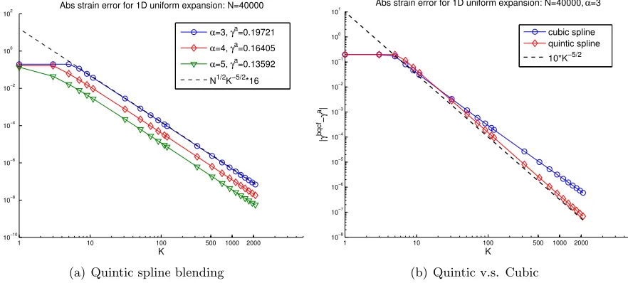
The computational results are shown in Figure 1. In Figure 1(a) we plot the dependence of the errors of quintic blending onK for different values ofα. We see that the graph of the error for the quintic blending is very close to the lower boundK−5/2 as given by (2.8) in Theorem 2.1. Also, the error is lower for larger α, which is also in accordance with the theoretical results. Indeed, whenα
is large, the strength of the next-nearest neighbor interaction,φ002F, is small relative to the nearest neighbor interaction φ00F, which contributes to a better stability of B-QCF according to (2.8).
Figure 1(b) shows the results of comparison of the cubic and the quintic blending. We see that the cubic blending produces the error that seems to decay slower, like K−2. On the other hand, the quantitative difference between cubic and quintic is not large on the example considered. To observe a significantly higher accuracy of the quintic spline, the computational domain sizeN has to be much larger. In addition, for larger α, N has to be even larger for the quintic blending to have advantage over the cubic blending.
3. The B-QCF Operator in 2D.
3.1. The Triangular Lattice. For some integer N ∈ N and := 1/N, we define the scaled 2D triangular latticeL to be
L:=A6Z2, where A6:= [a1, a2] :=
1 1/2 0 √3/2
,
where ai, i = 1,2 are the scaled lattice vectors. Throughout our analysis, we use the following definition of the periodic reference cell
Ω :=A6(−N/2, N/2]2 and L:=L∩Ω. We furthermore seta3 = (−1/2,
√
3/2)T, then the set ofnearest-neighbor directions is given by
1 10 100 500 1000 2000 10−10
10−8 10−6 10−4 10−2 100 102
K
|
γ
bqcf
−
γ
a|
Abs strain error for 1D uniform expansion: N=40000
α=3, γa=0.19721
α=4, γa=0.16405
α=5, γa=0.13592
N1/2K−5/2*16
(a) Quintic spline blending
1 10 100 500 1000 2000
10−8
10−7 10−6
10−5
10−4 10−3
10−2 10−1
100 101
K
|
γ
bqcf
−
γ
a|
Abs strain error for 1D uniform expansion: N=40000, α=3
cubic spline quintic spline 10*K−5/2
[image:8.612.88.529.115.314.2](b) Quintic v.s. Cubic
Figure 1. (a) The absolute critical strain errors for a 1D uniform expansion. We set N = 40,000, ∆γ = 1/N2 where ∆γ is the strain increment used for testing stability, and γa and γbqcf are the critical strains for the atomistic and B-QCF models, respectively. The dashed line corresponds to the theoretical asymptote. (b) The absolute critical strain errors of quintic and cubic blending functions with
N = 40,000 and α= 3. The solid line corresponds to the theoretical asymptote.
The set of next nearest-neighbor directions is given by
N2 :={±b1,±b2,±b3}, where b1 :=a1+a2, b2:=a2+a3, and b3 =a3−a1.
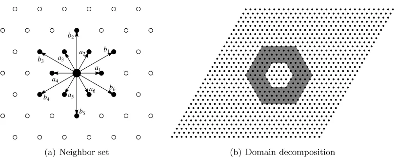
We use the notation N := N1 ∪ N2 to denote the directions of the neighboring bonds in the interaction range of each atom (see Figure 2).
We identify all lattice functions v:L→ R2 with their continuous, piecewise affine interpolants with respect to the canonical triangulation T of R2 with nodesL.
3.2. The Atomistic, Continuum, and Blending Regions. Let Hex(R) denote the closed hexagon centered at the origin, with sides aligned with the lattice directions a1, a2, a3, and di-ameter 2R. For Ra < Rb < N ∈ N, we define the atomistic, blending, and continuum regions, respectively, as
Ωa:=Hex(Ra), Ωb :=Hex(Rb)\Ωa, and Ωc:= clos (Ω\(Ωa∪Ωb)).
We denote the blending width by K := Rb −Ra. Moreover, we define the corresponding lattice sites
La:=L ∩Ωa, Lb :=L ∩Ωb, and Lc:=L ∩Ωc.
For simplicity, we will again use L as the finite element nodes, that is, every atom is a repatom. For a mapv:L→R2 and bond directions r, s∈ N, we define the finite difference operators
Drv(x) :=
v(x+r)−v(x)
and DrDsv(x) :=
Dsv(x+r)−Dsv(x)
a1
a2
a3
a4
a5
a6
b1
b2
b3
b4
b5
b6
[image:9.612.103.510.106.267.2](a) Neighbor set (b) Domain decomposition
Figure 2. (a) The 12 neighboring bonds of each atom. (b) The periodic reference cell L := L∩Ω, the atomistic region Ωa := Hex(Ra), and the blending region Ωb:=Hex(Rb)\Ωa. Here,N = 32, Ra= 3, Rb = 7, andK = 4.
We define the space of all admissible displacements, U, as all discrete functions L→ R2 which are Ω-periodic and satisfy the mean zero condition on the computational domain:
U :=nu:L→R2 :u(x) is Ω-periodic andPx∈Lu(x) = 0 o
.
For a given matrixB ∈R2×2, det(B)>0, we admit deformationsy from the space
YB :=
y:L→R2 :y(x) =Bx+u(x) ∀x∈L, for someu∈ U .
For a displacementu∈ Uand its discrete directional derivatives, we employ the weighted discrete
`2
and `∞ norms given by
kuk`2
:=
2X
x∈L |u(x)|2
!1/2
, kuk`∞
:= maxx∈L |u(x)|, and
kDuk`2
:=
2X
x∈L 3 X
i=1
|Daiu(x)|2 !1/2
.
The inner product associated with`2 is
hu,wi:=2X
x∈L
u(x)·w(x).
3.3. The B-QCF operator. The total scaled atomistic energy for a periodic computational cell Ω is
Ea(y) = 2
2 X
x∈L X
r∈N
φ(Dry(x)) =2 X
x∈L 3 X
i=1
φ(Daiy(x)) +φ(Dbiy(x))
, (3.1)
whereφ∈C2(R2), for the sake of simplicity. Typically, one assumesφ(r) =ϕ(|r|); the more general form we use gives rise to a simplified notation; see also [33]. We defineφ0(r)∈R2 andφ00(r)∈
The equilibrium equations are given by the force balance at each atom,
Fa(x;y) +f(x;y) = 0, for x∈ L, (3.2)
wheref(x;y) are the external forces andFa(x;y) are the atomistic forces (per unit area2)
Fa(x;y) :=− 1
2
∂Ea(y)
∂y(x)
=−1
3 X
i=1 h
φ0(Daiy(x)) +φ0(D−aiy(x)) i −1 3 X i=1 h
φ0(Dbiy(x)) +φ0(D−biy(x)) i
.
Again, since u = y−yB, where yB(x) = Bx, is assumed to be small, we linearize the atomistic equilibrium equation (3.2) about yB:
(Laua) (x) =f(x), for x∈ L,
where (Lau) (x), for a displacement u, is given by
(Lau) (x) =− 3 X
i=1
φ00(Bai)DaiDaiu(x−ai)− 3 X
i=1
φ00(Bbi)DbiDbiu(x−bi), for x∈ L.
We use the Cauchy-Born extrapolation rule to approximate the nonlocal atomistic model by a local continuum Cauchy-Born model [29, 39, 41]. Using the bond density lemma [33, Lemma 3.2] (see also [37]), we can write the total QCL energy (the discretized Cauchy-Born energy) as a sum of the bond density integrals
Ec(y) = 1 Ω0
Z
Ω X
r∈N
φ(∂ry)dx= X x∈L X r∈N Z 1 0
φ ∂ry(x+tr)
dt, (3.3)
where the factor Ω0:= √
3/2 is the volume of one primitive cell of Land ∂ry(x) := dtdy(x+tr)|t=0 denotes the directional derivative. We compute the continuum force
Fc(x;y) =−1
2
∂Ec
∂y(x),
and linearize the force equation about the uniform deformation yB to obtain
(Lcuc) (x) =f(x), for x∈ L.
To formulate the B-QCF method, we let the blending functionβ(s) :R2 →[0,1] be a “smooth”, Ω-periodic function. Then, the (nonlinear) B-QCF forces are given through a convex combination of Fa(x;y) and Fc(x;y):
Fbqcf(x;y) :=β(x)Fa(x;y) + (1−β(x))Fc(x;y),
and linearizing the equilibrium equation Fbqcf+f = 0 about yB yields
(Lbqcfubqcf)(x) =f(x), forx∈ L,
where (Lbqcfu)(x) =β(x)(Lau)(x) + (1−β(x))(Lcu)(x). (3.4)
The 2D blending function in our computational experiments will be defined radially using cubic and quintic splines:
ˆ
β(x) := ˆB
Rb− |x|
Rb−Ra
and β¯(x) := ¯B
Rb− |x|
Rb−Ra
where ˆB(x) is given by (2.10) and ¯B(x) is given by (2.11). The function ¯β(x) has the smoothness and satisfies 2D versions of the scaling bounds (2.5) needed for Theorem 3.1 below, whereas ˆβ(x) does not have a bounded third derivative. We therefore can expect that ˆβ(x) will give a larger error asymptotically as compared to ¯β(x).
3.4. Positivity of the B-QCF operator in 2D. Necessary and sufficient conditions forLbqcf to be positive-definite are given in [21]. To make this paper more concise, we only state the conclusions without proof. First, we state a lower bound for hLbqcfu,ui:
Theorem 3.1. Suppose thatβ ∈C3 and satisfies the scaling bounds (2.5); then,
hLbqcfu,ui ≥γbqcfkDuk2`2
,
where
γbqcf := ˜γ−C
K−5/2R1b/2|log(Rb/N)|1/2
, (3.5)
where C is a generic constant independent of N, and γ˜ is the coercivity constant for the operator ˜
L:
hL˜u,ui:=hLcu,ui −4
3 X
i=1 X
x∈L
β(x−a2)
DaiDai+1u(x−a1−a2) 2
bi ≥γ˜kDuk 2 `2
∀u∈ U.
One can see very clearly that, wheneverN is polynomial inRb andK R1b/5, thenLbqcf can be expected to be coercive. Both are natural and easy to achieve. We can thus deduce the following result for the coercivity ofLbqcf :
Corollary 3.1. Suppose that L˜ is positive-definite and that the blending function β ∈ C3 and satisfies the scaling bounds (2.5). Let the number of atomsRa along the radius be of orderNα with 0≤α≤1. If the blending width K satisfies
K
|logN|1/4, α= 0,
|logN|1/5Nα/5, 0< α <1,
N1/5, α= 1,
then the B-QCF operator Lbqcf is positive-definite.
Remark 3.1.
(a) The stability result of Theorem 3.1, and hence of Corollary 3.1, is based on the conjecture that the operator ˜L is stable. In [21] we show that ˜L is indeed stable whenever nearest-neighbor interactions dominate.
Moreover, based on the analysis and numerical experiments in [33] for a similar linearized operator, we expect that the region of stability for ˜Lis the same as forLaasN, Ra, Rb → ∞. We therefore expect that the result of Theorem 3.1 holds (up to a controllable error) if coercivity of ˜Lis replaced by coercivity ofLa in the hypothesis.
(b) One can apply the argument of Remark 2.1 to conclude that the results of Theorem 3.1 and Corollary 3.1 are valid for homogeneous Dirichlet boundary conditions as well.
Theorem 3.2. Suppose that La is positive-definite and that the blending function β ∈ C3 and satisfies the scaling bounds (2.5). The number of atoms Ra along the radius is of order Nα with 0 < α ≤ 1. If the blending width K is K Nα/5, then the B-QCF operator Lbqcf cannot be positive-definite and we can construct a radial counterexample in this case.
We note that there is a gap between the necessary and sufficient conditions for 0 < α < 1. In addition, we have no necessary condition for α = 0, which corresponds to a fixed atomistic core independent of the reference cell Ω.
3.5. 2D numerical experiments for B-QCF operators. In this subsection, we will continue the numerical experiments for the 2D B-QCF models to verify the theoretical findings by comparing the decay rates of the error in critical strain as computed by B-QCF with the theoretically predicted rates as we increase the blending widthK.
(1) Uniform expansion.
We first consider the simplest 2D deformation: we apply a uniform expansiony(x) =Bx
with
B =γ
1 0
0 1
to the perfect lattice L with Dirichlet boundary condition:
u(x) = 0 ∀x∈∂Ω. (3.6)
Then we compute the critical strains γ of the atomistic and B-QCF models with different blending region width K.
We note that the 2D conclusions also depend on the size of the atomistic region. Therefore we let Ra=K5/3 in order to narrow the dependence only to the blending width K. Then the asymptotical term in (3.5) for sufficiently large N is approximately
K−5/2R1b/2|log(Rb/N)|1/2=K−5/2(Ra+K)1/2|log(Rb/N)|1/2
≈K−5/2R1a/2 =K−5/3=R−a1,
which means that the error in γbqcf is systematically improvable.
The choice of scaling Ra =K5/3 is motivated by the results in [17] which indicate that, generically, one should expect an O(R−a1) error in the regions of stability between the infinite lattice atomistic model and the atomistic model in a domain with radius Ra. In the computation, we assign integer values forK and use the rounded values forRa, that is
Ra=bK5/3c.
The critical strains are defined as
γw:= max¯γ >0 :Lw(Bx) is positive definite forγ ∈[0,γ¯) , (3.7)
where w ∈ {a,bqcf} denote the models. Here we use the MATLAB function eigs [28] to compute the smallest eigenvalue of the symmetric part of Lw(Bx) and thus determine the positive-definiteness of Lw(Bx).
We also define the increment of the strain γ in each step by ∆γ. The results in [10, 14, 17, 33] suggest that the theoretical increments be of orderO(N−2) (at least, for finding the critical strain of a uniform lattice), and we set ∆γ = 10−8 which is sufficiently small considering N = 200 or 300 in our experiments.
We plot the difference of the critical strains with different blending widthK in Figure 3. The numerical critical strain errors in the left figure approach the analytical asymptote as
1 5 10 15 20 25 10−4
10−3 10−2 10−1
K
|
γ
bqcf
−
γ
a|
Abs strain error for 2D uniform expansion: N=500, Ra=K5/3
α=3, γa=0.1838
α=4, γa=0.1589
α=5, γa=0.1355 K−5/2|Rb/N*ln(Rb/N)|1/2
(a) Quintic spline blending
1 5 10 15 20 25
10−3 10−2 10−1
K
|
γ
bqcf
−
γ
a|
Abs strain error for 2D uniform expansion: N=500, Ra=K5/3,α=3
cubic spline quintic spline
K−5/2|Rb/N*ln(Rb/N)|1/2*1.3
[image:13.612.86.529.114.318.2](b) Quintic v.s. Cubic
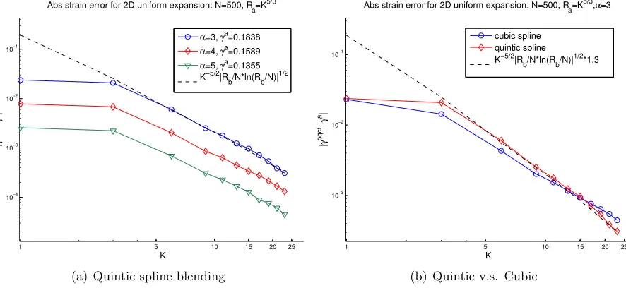
Figure 3. (a) The absolute critical strain errors for the 2D uniform expansion. We set N = 500, and we denote the critical strains for the atomistic and B-QCF models byγa andγbqcf,respectively. The dashed line corresponds to the theoretical asymptote. (b) The absolute critical strain errors for the quintic and cubic blending functions with N = 500 and α = 3. The solid line corresponds to the theoretical asymptote.
likely due to round-off errors in calculating Ra=K5/3. Thus, the slopes of the errors with quintic blending agree with the theoretical prediction in Theorem 3.1. Also, similarly to the 1D results, the error is smaller when the nearest neighbor interaction dominates (that is, when α is large).
Although the slope of the errors with cubic blending seems to be one half order less than that with quintic blending (see Figure 3(b)), the computed errors for cubic blending are slightly smaller for the relatively smallN considered. We expect that for a sufficiently large system, the quintic blending would be more accurate. In addition, the 2D errors for uniform expansion are similar to the 1D results. This is reasonable since the 2D uniform expansion is similar to the 1D deformation.
(2) Uniform shear deformation.
We now investigate stability of B-QCF under shear deformation. We apply a y-directional shear deformation to the hexagonal lattice Ω with Dirichlet boundary conditions (3.6). The y-directional shear is y(x) = ˜Bxwith
˜
B =
1 0
γ 1
.
The critical strain errors between the B-QCF and atomistic models with the quintic blending are plotted in Figure 4.
In Figure 4 we plot the critical strain errors in the following three regimes: (1)N increases,
Ra = const, K = const, (2) all three parameters increase, and (3) N = const, Ra and
40 80 120 160 200 10−2.8
10−2.7 10−2.6 10−2.5 10−2.4 10−2.3 10−2.2
Rel error for y−shear with quintic spline: α=4
N
|
γ
bqcf
−
γ
a|/
γ
a
K=2, Ra=14
K=N3/10, Ra=N1/2
10−1/2N−1
(a) Error vsN
4 5 7 9
10−2.8 10−2.7 10−2.6
Ra
|
γ
bqcf
−
γ
a|/
γ
a
Rel error for y−shear with quintic spline: α=4
N=200, K=R
a 3/5
10−5N−1
[image:14.612.89.523.113.304.2](b) Error vsRa
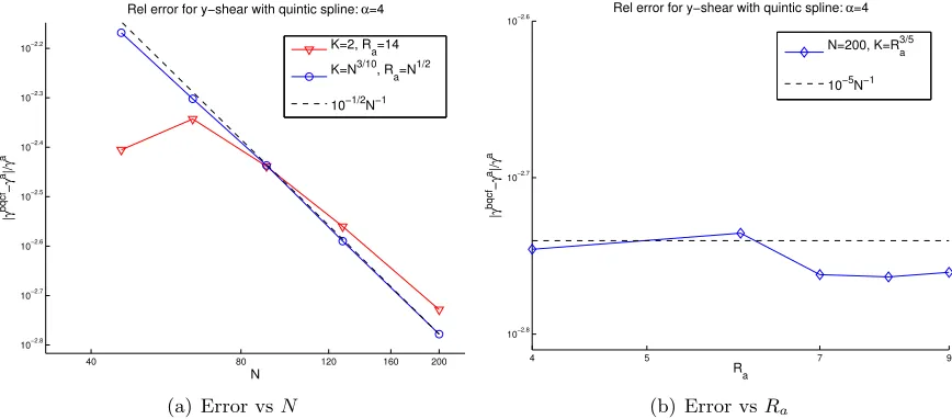
Figure 4. The relative critical strain error for the y-directional shear deformation.
γaandγbqcfare the critical strains for the atomistic and B-QCF models respectively. ForN = 200,γa≈0.1813.The dashed line corresponds to the theoretical asymptote. The fluctuations in the plotted error for N = const seems to be due to round-off errors in calculating Ra and K. The method parameters were rounded as follows: in (a)K =bN3/10c and Ra =bN1/2c, and in (b)K =bR
3/5 a c.
significantly affect the results in this case. The results indicate that the error in this case depends on N, but does not depend onRaorK. This means that, for shear deformations, the local continuum approximation and its finite element coarse-graining contributes most of the error.
We explain such a qualitative difference between the uniform expansion and the shear deformation in the following way. For the uniform expansion the onset of instability is due to competition of interaction of the nearest neighbors (NNs), contributing to stability, and the second nearest neighbors (NNNs), contributing to instability. On the other hand, for the shear deformation the onset of instability is primarily due to competition between elongated and compressed NN bonds. Therefore, for the uniform expansion it is important to reduce the interface error which distorts the NNN interaction, whereas in shear defor-mation the NNN interactions do not contribute significantly to stability errors. Since, for NN interaction, the atomistic, Cauchy-Born and B-QCF models are identical, the stability error only depends on the domain size.
(3) Regions of stability.
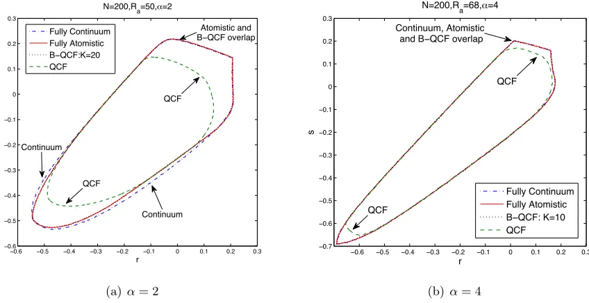
We now combine the uniform expansion and shear deformation together and study the stability region of Lbqcf for a general class of homogeneous deformations. We consider the following family of deformations which involve shear, expansion, and compression.
B =
1 +s 0.1
0 1 +r
.
−0.6 −0.5 −0.4 −0.3 −0.2 −0.1 0 0.1 0.2 0.3 −0.6
−0.5 −0.4 −0.3 −0.2 −0.1 0 0.1 0.2 0.3
r
s
N=200,Ra=50, =2
Fully Continuum Fully Atomistic
B−QCF:K=20
QCF
Continuum
Continuum QCF
QCF
Atomistic and
B−QCF overlap
(a)α= 2
−0.6 −0.5 −0.4 −0.3 −0.2 −0.1 0 0.1 0.2 0.3
−0.7 −0.6 −0.5 −0.4 −0.3 −0.2 −0.1 0 0.1 0.2 0.3
r
s
N=200,R
a=68, =4
Fully Continuum Fully Atomistic
B−QCF: K=10
QCF Continuum, Atomistic
and B−QCF overlap
QCF
QCF
[image:15.612.92.516.112.330.2](b)α= 4
Figure 5. The stability regions of the different models. These closed curves are the boundaries of the stability regions for the atomistic, B-QCF, and the local continuum models, respectively. The curves with indicators are for QCF.
We observe that the stability regions of the B-QCF model with different blending sizes are all proper subsets of the atomistic model. In addition, the fully atomistic and continuum models are very close to each other, which agrees with the stability analysis of the perfect lattice [17]. Also, when α increases, which means the next-nearest neighbor interactions become less important, the difference becomes smaller.
There is a visible difference in the stability regions between the QCF model and the exact atomistic model, whereas the difference between the B-QCF model and the atomistic model is almost not seen. This implies that using a blending region can significantly improve the stability properties of the approximation models.
(4) Stability of micro-cracks.
The experiments that we have reported up to this point were based on perfect lattices. Now we apply the B-QCF model to lattices with local defects.
The atomistic system is as follows. There is a micro-crack in the center of the domain Ω with length 5, i.e., 5 atoms are removed from the lattice (see Figure 6). Hence, we redefine accordingly the positions of atoms in the reference configuration x, the interaction energy
Ea, etc. We impose a vertical stretchingB =
1 0
0 1 +γ
on the lattice and compute the
critical strains γc>0 beyond which the system loses stability.
We computed the critical strain γc in the following way. Given γ >0, we use Newton’s iteration method to solve the following force equations foryγwith the initial guessyF =Bx:
Fw(x;yγ) = 0 for x∈Ω\∂Ω.
−8 −6 −4 −2 0 2 4 6 8 −2
−1 0 1 2 3
[image:16.612.131.492.114.237.2]Equilibrium of crack−5 with γ=0.001
Figure 6. The stable equilibrium configuration of the micro-crack with crack length= 5 andγ = 0.001, and the`∞ norm of the force residual is of orderO(10−12).
residual to be less than 100 and the positive-definiteness of Lw(y), wherey is the current configuration. If any of the two requirements is not met, then the current γ is regarded as an unstable strain. When the force residual is smaller than the tolerance, the configuration y∗ is thought to be in its equilibrium of the local energy well. Then we check the positive definiteness of corresponding operator Lw(y∗) with the equilibrium configuration y∗. The nonlinear critical strain is thus defined as
γc:= max{γ >¯ 0 :Lw(y∗) is positive definite forγ ∈[0,γ¯)}.
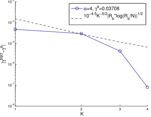
The plot of critical strain for the B-QCF models are shown in Figure 7. Even though we
1 2 3 4
10−8 10−7 10−6 10−5 10−4 10−3
K
|
γ
bqcf
−
γ
a |
α=4, γa=0.03708
10−4.5K−5/2|R
b*log(Rb/N)|
1/2
Figure 7. The nonlinear critical strain error for vertical stretching. We set N = 200, crack length= 5, and Ra = max{K2,6}. γa, γbqcf are the critical strains for the atomistic and B-QCF models, respectively. The dashed line corresponds to the theoretical asymptote.
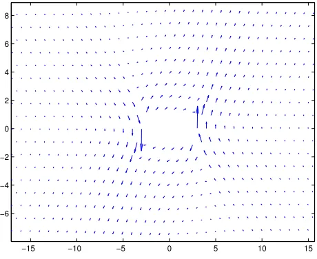
[image:16.612.176.427.434.628.2]−15 −10 −5 0 5 10 15 −6
[image:17.612.193.423.122.310.2]−4 −2 0 2 4 6 8
Figure 8. The zoomed-in critical eigenvector of critical strain of vertically stretch-ing a micro-crack. We setN = 200, crack length= 5, strain increment ∆γ = 10−11 and α= 4.
we observe the nonlinear error decays much faster than the theoretical predicted rates and it can reach the strain increment ∆γ = 10−8. This phenomenon has been observed in [33] and is likely related to superconvergence of local quantities of interest. The indicator of the superconvergence is the concentration of the critical eigenmode corresponding to γc near the defect, which is illustrated in Figure 8.
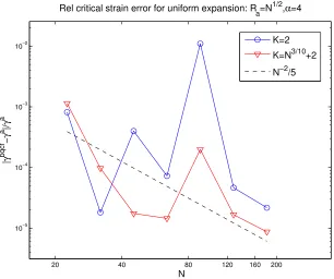
We also study the relative errors of the critical strains for two different choices of the blending width, K = 2 and K ≈ R3a/5+ 2. Motivated by the analysis in [33], the size of the atomistic core is chosen to beRa=
√
N. According to Figure 9, the relative errors for
K ≈R3a/5+ 2 are approximately 10 times smaller than those for K = 2. But both graphs decay rapidly as N increases. The rate of decay appears to be quadratic.
Remark 3.2. The numerical computations in this section are conducted without coarsening. The main reason for this was that coarsening introduces more approximation parameters and potentially more fluctuations in the results. Typically, coarsening does not reduce the stability, and we therefore expect that our stability results will remain valid for any coarsening. Another reason to discard coarsening was to better compare the numerics with the theory. However, the purpose of a/c coupling is to reduce the number of degrees of freedom of an atomistic computation, therefore coarsening is required when comparing efficiency (i.e., accuracy against the number of degrees of freedom) of different methods.
4. The Accuracy of B-QCF
20 40 80 120 160 200
10−5
10−4
10−3
10−2
N
|
γ
bqcf
−
γ
a |/
γ
a
Rel critical strain error for uniform expansion: R
a=N 1/2,α=4
K=2
K=N3/10+2
[image:18.612.154.460.113.369.2]N−2/5
Figure 9. The relative errors of the critical strains of vertically stretching a micro-crack in log10scale plot. We set crack length= 5 andα= 4. γa,γbqcf are the critical strains for the atomistic and B-QCF models, respectively. The dashed line is the theoretical asymptote.
4.1. Implementation of the B-QCF method. LetV ⊂L be a set of vacancy sites and LV := L\ V the corresponding lattice with defects. Let B ∈ R2×2 be the applied far-field strain. We consider the atomistic problem
ya ∈arg minEa(y) :y:LV →R2, y(x)∼Bxas|ξ| → ∞ . (4.1)
We remark that one must carefully renormalizeEain order to rigorously make sense of this problem; see e.g. [19] for the details. The vacancy sites are accounted for in the definition of Ea by simply removing the relevant pair interactions.
We wish to approximate this problem with a practical variant (i.e., with coarsening) of the B-QCF method. To that end, we chooseRa, Rb=Ra+K, N ∈Nin such a way that all vacancy sites are contained in the atomistic region Ωa, which is a hexagon with side length Ra. The blending region is defined analogously. The full computational domain is given by Ω, which is a hexagon with side lengthN. We triangulate Ω in such a way that it matches the canonical triangulation of the triangular lattice in Ω.
LetTh denote the set of triangles, letNh denote the nodes of the triangulation, and letNhfree := Nh\(V ∪∂Ω) denote the free nodes.
Let P1h denote the space of all functions vh : Ω→ R2, that are continuous and piecewise affine with respect to the triangulation Th. The space of admissible trial functions is then given by
Yh:=
Each deformation yh∈Yh is understood to be extended byBxoutside of Ω and thereby gives rise to an admissible atomistic configuration.
We define the discretized Cauchy-Born energy functional as
Ec(yh) := X
T∈Th
vol(T)W ∇yh|T
,
where vol(T) in 2D is the area of the triangle T. We can define the discretized B-QCF operator, for a given blending function β, as follows:
Fbqcf(x;yh) := (1−β(x))
∂Ea(y)
∂y(x)
y=yh+β(x)
∂Ec(z h)
∂zh(x)
zh=yh forx
∈ Nfree
h .
In the B-QCF method, we aim to find a solution ybqcfh ∈Yh satisfying
Fbqcf(x;yhbqcf) = 0 ∀x∈ Nhfree. (4.2)
We remark that this method has essentially five approximation parameters that must be chosen carefully: the atomistic region size Ra, the blending width K, the computational domain size N, the blending function β,and the finite element meshTh.
4.1.1. Practical considerations. To implement (4.2) in practice, we need to specify further details of the method:
(1) In our choice of blending function, we deviate from the optimal choice of a C2,1-blending function and instead choose only aC1,1blending function, which is more easily constructed. This is justified, firstly, by our foregoing numerical experiments which suggest that little additional accuracy in the stability regions can be gained in the pre-asymptotic regime by using quintic splines (i.e., C2,1-blending), and secondly, because the consistency error does not depend on the regularity of the blending function.
We choose the blending function proposed in [27], which minimizesk∇2βk
L2, or a discrete variant thereof, in a precomputation step (see [27] for the details).
(2) In addition to the blending region Ωbwe ensure that two additional “layers” of atoms outside of it belong to Nh. This makes the implementation of the atomistic force contribution in (4.2) straightforward.
Moreover, we ensure that the vacancy sites do not affect the forces on atoms x where
β(x)6= 0. This ensures that all the Cauchy-Born force contributions in (4.2) are the correct Cauchy-Born forces.
(3) To obtain an appropriate initial guess for the B-QCF solutions, we first solve the corre-sponding energy-based blended QCE method (B-QCE) [27] with the same approximation parameters, using a preconditioned line search method. The details are described in [27]. The B-QCE solution is then taken as a starting guess for the B-QCF Newton iteration to solve (4.2). If no B-QCE code is readily available, then a natural alternative would be to implement a damped Newton method for B-QCF.
We remark, that the Jacobian matrix of the B-QCF operator is straightforward to as-semble from the Hessians of the atomistic and Cauchy-Born energy. Nevertheless, for large 3D simulations, more sophisticated solution methods may be required.
4.2. Error versus computational cost. We briefly review the main ideas of our analysis in [19] without technical details. A first key result is that if the atomistic solution is stable (δ2Ea(ya) is positive definite) and the linearized B-QCF operatorδFbqcf(·;Bx) is positive definite, then choosing
Ra and K sufficiently large implies that δFbqcf(·;ya) is also positive definite, that is, the B-QCF method is stableunder these conditions. To achieve this in practice, we need to choose K3 Ra (recall from section 4.1.1 that we have chosen a sub-optimal β).
From this stability result, we can deduce the existence of a B-QCF solution in a neighborhood of the atomistic solution, and an error estimate in terms of the best approximation error (the best approximation of ya from the finite element space Yh). and of the modeling error (the force discrepancy of the B-QCF and atomistic models). We estimate the error in the strain∇ya− ∇ybqcf
h in terms of the “smoothness” ofya, which is measured in terms of bounds on the derivatives∇jya. The derivatives of the discrete functions ya are understood as derivatives of a smooth interpolant. (See [19] for the details.)
Dropping an unimportant term for the sake of readability, our error estimate reads
k∇ya− ∇ybqcfh kL2(
R2) .C
stabCβk∇3yak L2(
R2\ωa)+kh∇ 2yak
L2(Ω\ω
a)+k∇y ak
L2(
R2\ω)
, (4.3)
wherek∇3yak L2(
R2\ωa) measures the modeling error,kh∇ 2yak
L2(Ω\ω
a) the finite element discretiza-tion error andk∇yakL2(
R2\ω) the error in the far-field due to the artificial boundary condition (the two latter errors comprise the best approximation error). The domains ωa, ω are slightly smaller hexagonal subsets of, respectively, Ωa and Ω, with comparable side lengths.
In addition,Cstab is a stability constant that is uniformly bounded forRaK3, and
Cβ :=K−1/2Ra1/2logRa/N
is aβ-dependent prefactor, which arises from a crucial inequality,k∇(βv)kL2 ≤Cβk∇vkL2, in the consistency analysis of B-QCF.
We choose K ≈ Ra and N a polynomial of Ra (we will see momentarily why this is natural), thenCβ is uniformly bounded and in addition, we chooseRaK3 , which we require for stability. With this choice, it is easy to see that Cβk∇3yak
L2(
R2\ωa) . kh∇ 2yak
L2(Ω\ω
a) (recall that we are working in units where atomic spacing is 1), and hence we can simply ignore the modeling error term from now on.
We recall from [27] that the atomistic method (ATM) is given by the B-QCF method withβ ≡0.
We also recall the corresponding error estimates (dropping less important terms) for the atomistic (ATM) and the B-QCE methods [19, 27]
k∇ya− ∇yatmkL2(
R2) .k∇y
ak L2(
R2\ω), (4.4)
k∇ya− ∇ybqceh kL2(
R2) .k∇2βkL2(
R2\ωa)+kh∇ 2yak
L2(Ω\ω
a)+k∇y ak
L2(
R2\ω). (4.5) To better understand the best approximation error, we need to understand the regularity of ya. Since the problems only involve defects with zero Burgers vector, it is reasonable to assume based on linear elasticity, that
|∇jya(x)| ∼ |x|−j−1.
(We stress that this estimate only applies in the far-field. In the preasymptotic regime different rates of decay might be observed, e.g., |∇jya(x)| ∼ |x|1/2−j for the micro-crack case discussed in§ 4.3.2.)
in [27], we obtain a triangulationTh (as a function of Rb and N), for which the following estimate holds:
kh∇2yakL2(Ω\ω
a)+k∇y ak
L2(
R2\ω) .R
−2
a +N
−1.
Thus, we chooseN ≈R2a to balance these two error contributions.
Finally, we note that, with this construction, the number of degrees of freedom in Yh, DoF := dimYh = 2#Nhfree is approximately equal to DoF ≈R2a. (In particular, the number of degrees of freedom in the atomistic, blending and continuum regions are comparable.)
In summary, choosing K ≈Ra, N ≈R2a, the blending function β according to the construction proposed in [27], and the finite element mesh according to the construction proposed in [33], we obtain from (4.3) the error estimate
k∇ya− ∇yhbqcfkL2(
R2).DoF
−1. (4.6)
We note thatN =Ra in the ATM method, and consequently we obtain from (4.5)
k∇ya− ∇yatmkL2(
R2).DoF
−1/2; (4.7)
thus demonstrating an improved rate of convergence for the B-QCF method in comparison with the ATM method.
We remark that this is optimal for P1-finite element type coarse-graining schemes, as the mod-eling error is in fact dominated by the finite element error. In particular, it is a substantial improvement over the B-QCE method, for which the corresponding error estimate obtained from (4.4) is
k∇ya− ∇yhbqcekL2(
R2).DoF
−1/2.
We note that the B-QCE method can be shown to have a higher rate of convergence than the ATM method for defects with nonzero Burgers vector (such as dislocations) which have a lower rate of decay. The finite element coarse-graining of the B-QCE method can more efficiently approximate the larger region where the strain gradient is significant; [19, 27] for the details.
4.3. Numerical rates. We test our analytical predictions against the two numerical examples, for which we already tested the B-QCE method in [27]. In both examples, we choose the Morse interaction potential
φ(r) = [1−exp(−α(r−1))]2,
with stiffness parameter α= 4.
We compare the B-QCF method with a pure atomistic computation on a finite domain, with the QCE and B-QCE methods (cf. [27] for a detailed description of these three methods) and with the pure QCF method, which is simply the B-QCF method withK <1 (i.e., β(x)∈ {0,1}).
Finally, we have also included a highly optimized B-QCE variant where we choose K ≈ R2a
and N ≈R4
a, which is a very unexpected scaling, but yields improved errors in the preasymptotic regime; see [27, Remark 4.3]. We denote this method by B-QCE+ in the error graphs.
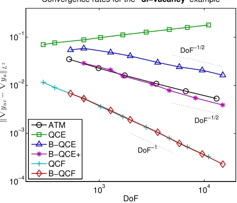
4.3.1. The di-vacancy example. We choose the vacancy set V ={0, e1} and the macroscopic strain
B =
1.03 0.3 0.0 1.03
·B0,
whereB0 is a minimizer of W (3% uniform stretch and 3% shear from ground state). The setup of the B-QCF method for the di-vacancy problem is shown in Figure 10.
−100 −50 0 50 100 −100
−50 0 50 100
−10 −5 0 5 10
[image:22.612.111.502.117.276.2]−10 −5 0 5 10
Figure 10. Setup of the B-QCF method for the di-vacancy example, for a specific choice of approximation parameters, shown in deformed equilibrium. The size/color of the atoms in the center correspond to decreasing values of (1−β(x)).
103 104
10−4
10−3
10−2
10−1
DoF
k
∇
ya
c
−
∇
ya
kL
2
Convergence rates for the di−vacancy example
ATM QCE B−QCE B−QCE+ QCF B−QCF
DoF−1
DoF−1/2
DoF−1/2
Figure 11. Plots of computational cost (DoF) versus error in the energy-norm for various a/c coupling methods approximating the di-vacancy problem described in section 4.3.1.
barely distinguishable from the B-QCF method in this graph. Unfortunately, we cannot offer a satisfactory theory for the QCF method at present.
[image:22.612.185.422.357.560.2]−100 −50 0 50 100 −100
−50 0 50 100
0 5 10 15 20 25
[image:23.612.109.505.115.276.2]−10 −5 0 5 10
Figure 12. Setup of the B-QCF method for the micro-crack example, for a specific choice of approximation parameters, shown in deformed equilibrium. The size/color of the atoms in the center correspond to decreasing values of (1−β(x)).
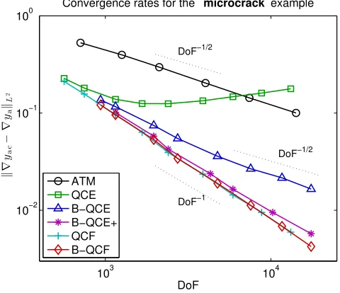
103 104
10−2
10−1
100
DoF
k
∇
ya
c
−
∇
ya
kL
2
Convergence rates for the microcrack example
ATM QCE B−QCE B−QCE+ QCF B−QCF
DoF−1 DoF−1/2
DoF−1/2
Figure 13. Plots of computational cost (DoF) versus error in the energy-norm for various a/c coupling methods approximating the micro-crack problem described in section 4.3.2.
4.3.2. The micro-crack example. In the micro-crack (or void) example, we choose the vacancy set V ={−5e1, . . . ,5e1} and the macroscopic strain
B =
1.0 0.03 0.0 1.03
·B0,
[image:23.612.183.423.354.561.2]In Figure 13 we plot the degrees of freedom (DoF) against the error in the energy-norm, for the various a/c coupling methods that we consider. In this example the picture is less clear than in the di-vacancy example due to a more significant preasymptotic regime, which is caused by the more significant deformation admitted by the microcrack. In the preasymptotic regime we observe that the QCE and B-QCE methods perform much better than expected, but eventually fall back to the predicted rates. By contrast, the B-QCF and QCF methods display clear systematic convergence at the predicted rate throughout.
We also note that, in this example, the B-QCE+ method performs comparable to the B-QCF and QCF methods, at least in the preasymptotic regime accessible in the experiment.
5. Conclusion
We have formulated an atomistic-to-continuum force-based coupling, which we call the blended force-based quasicontinuum (B-QCF) method. In this paper, we numerically studied the stability as well as accuracy of the B-QCF method. We computed the critical strain errors between the atomistic and B-QCF models with different sizes of the blending region under different types of deformations.
The main theoretical conclusion in [21] is that the required blending width to ensure coercivity of the linearized B-QCF operator is surprisingly small. For both 1D and 2D uniform expansion, the computational results of the linearized operators perfectly match the analytic predictions. In addition, the stability for a general class of homogeneous deformations of the 2D B-QCF operator becomes almost the same as that of the atomistic model by using a very small blending region, in contrast to the fact that the stability region of the force-based quasicontinuum (QCF) method, that is, the B-QCF method without blending region, is just a proper subset of the fully atomistic model. However, the critical strain error for the B-QCF operator applied to shear deformation seems to only linearly depend on the system size and is thus insensitive to blending width.
For the problem of a microcrack in a two-dimensional crystal, we studied the nonlinear stability of the B-QCF operators. The critical strain error decays faster than the prediction, and it can be as small as the strain increment. However, we find that the error increases a little bit when the blending size becomes larger, which is possibly due to round-off error.
Moreover, we implemented a practical version of the B-QCF method. We briefly reviewed the accuracy results in terms of computational cost [19]. The numerical experiments, di-vacancy and microcrack demonstrate the superior accuracy of B-QCF over other a/c coupling schemes that we have investigated previously in [27].
The BQCF method with a surprisingly small blending region is an appealing choice for numerical simulations of atomistic multi-scale problems as it is always consistent and can be guaranteed by both theory and benchmark testing to be positive definite when the fully atomistic operator is positive definite.
6. Acknowledgments
We appreciate helpful discussions with Brian Van Koten.
References
[1] S. Badia, P. Bochev, R. Lehoucq, M. L. Parks, J. Fish, M. Nuggehally, and M. Gunzburger. A force-based blend-ing model for atomistic-to-continuum couplblend-ing.International Journal for Multiscale Computational Engineering, 5:387–406, 2007.
[3] P. T. Bauman, H. B. Dhia, N. Elkhodja, J. T. Oden, and S. Prudhomme. On the application of the Arlequin method to the coupling of particle and continuum models.Comput. Mech., 42(4):511–530, 2008.
[4] T. Belytschko and S. P. Xiao. Coupling methods for continuum model with molecular model. International Journal for Multiscale Computational Engineering, 1:115–126, 2003.
[5] T. Belytschko, S. P. Xiao, G. C. Schatz, and R. S. Ruoff. Atomistic simulations of nanotube fracture.Phys. Rev B, 65, 2002.
[6] X. Blanc, C. Le Bris, and F. Legoll. Analysis of a prototypical multiscale method coupling atomistic and con-tinuum mechanics.M2AN Math. Model. Numer. Anal., 39(4):797–826, 2005.
[7] W. Curtin and R. Miller. Atomistic/continuum coupling in computational materials science. Modell. Simul. Mater. Sci. Eng., 11(3):R33–R68, 2003.
[8] M. Dobson and M. Luskin. Analysis of a force-based quasicontinuum approximation.M2AN Math. Model. Numer. Anal., 42(1):113–139, 2008.
[9] M. Dobson and M. Luskin. An analysis of the effect of ghost force oscillation on the quasicontinuum error. Mathematical Modelling and Numerical Analysis, 43:591–604, 2009.
[10] M. Dobson, M. Luskin, and C. Ortner. Accuracy of quasicontinuum approximations near instabilities.Journal of the Mechanics and Physics of Solids, 58:1741–1757, 2010.
[11] M. Dobson, M. Luskin, and C. Ortner. Sharp stability estimates for force-based quasicontinuum methods.SIAM J. Multiscale Modeling and Simulation, 8:782–802, 2010.
[12] M. Dobson, M. Luskin, and C. Ortner. Stability, instability and error of the force-based quasicontinuum approx-imation.Archive for Rational Mechanics and Analysis, 197:179–202, 2010.
[13] M. Dobson, M. Luskin, and C. Ortner. Iterative methods for the force-based quasicontinuum approximation. Computer Methods in Applied Mechanics and Engineering, 200:2697–2709, 2011.
[14] M. Dobson, C. Ortner, and A. V. Shapeev. The Spectrum of the Force-Based Quasicontinuum Operator for a Homogeneous Periodic Chain.Multiscale Model. Simul., 10(3):744–765, 2012.
[15] W. E, J. Lu, and J. Yang. Uniform accuracy of the quasicontinuum method.Phys. Rev. B, 74(21):214115, 2006. [16] J. Fish, M. A. Nuggehally, M. S. Shephard, C. R. Picu, S. Badia, M. L. Parks, and M. Gunzburger. Concurrent AtC coupling based on a blend of the continuum stress and the atomistic force.Comput. Methods Appl. Mech. Engrg., 196(45-48):4548–4560, 2007.
[17] T. Hudson and C. Ortner. On the stability of Bravais lattices and their Cauchy–Born approximations.M2AN Math. Model. Numer. Anal., 46:81–110, 2012.
[18] B. V. Koten and M. Luskin. Analysis of energy-based blended quasicontinuum approximations.SIAM. J. Numer. Anal., 49:2182–2209, 2011.
[19] H. Li, M. Luskin, C. Ortner, A. V. Shapeev, and B. Van Koten. Blended atomistic/continuum hybrid methods. manuscript.
[20] X. H. Li and M. Luskin. A generalized quasi-nonlocal atomistic-to-continuum coupling method with finite range interaction.IMA Journal of Numerical Analysis, 32:373–393, 2012.
[21] X. H. Li, M. Luskin, and C. Ortner. Positive-definiteness of the blended force-based quasicontinuum method. SIAM J. Multiscale Modeling & Simulation, 10:1023–1045, 2012. arXiv:1112.2528v1.
[22] P. Lin. Convergence analysis of a quasi-continuum approximation for a two-dimensional material without defects. SIAM J. Numer. Anal., 45(1):313–332 (electronic), 2007.
[23] W. K. Liu, H. Park, D. Qian, E. G. Karpov, H. Kadowaki, and G. J. Wagner. Bridging scale methods for nanomechanics and materials.Comput. Methods Appl. Mech. Engrg., 195:1407–1421, 2006.
[24] J. Lu and P. Ming. Stability of a force-based hybrid method in three dimension with sharp interface.ArXiv e-prints, Dec. 2012.
[25] J. Lu and P. Ming. Convergence of a force-based hybrid method in three dimensions.Communications on Pure and Applied Mathematics, 66(1):83–108, 2013.
[26] M. Luskin and C. Ortner. Atomistic-to-continuum coupling.Acta Numerica, 22:397–508, 4 2013.
[27] M. Luskin, C. Ortner, and B. Van Koten. Formulation and optimization of the energy-based blended quasicontin-uum method.Computer Methods in Applied Mechanics and Engineering, 253:160–168, 2013. arXiv: 1112.2377. [28] MATLAB.version 8 (R2012b). The MathWorks Inc., Natick, Massachusetts, 2010.
[29] R. Miller and E. Tadmor. The quasicontinuum method: overview, applications and current directions.Journal of Computer-Aided Materials Design, 9:203–239, 2003.
[31] P. Ming and J. Z. Yang. Analysis of a one-dimensional nonlocal quasi-continuum method. Multiscale Model. Simul., 7(4):1838–1875, 2009.
[32] C. Ortner. A priori and a posteriori analysis of the quasinonlocal quasicontinuum method in 1D.Math. Comp., 80(275):1265–1285, 2011.
[33] C. Ortner and A. V. Shapeev. Analysis of an energy-based atomistic/continuum approximation of a vacancy in the 2D triangular lattice.Math. Comp., 82:2191–2236, 2013. arXiv:1104.0311.
[34] C. Ortner and L. Zhang. Construction and sharp consistency estimates for atomistic/continuum coupling methods with general interfaces: a 2D model problem.SIAM J. Numer. Anal., 50, 2012.
[35] S. Prudhomme, H. Ben Dhia, P. T. Bauman, N. Elkhodja, and J. T. Oden. Computational analysis of modeling error for the coupling of particle and continuum models by the Arlequin method.Comput. Methods Appl. Mech. Engrg., 197(41-42):3399–3409, 2008.
[36] P. Seleson and M. Gunzburger. Bridging methods for atomistic-to-continuum coupling and their implementation. Communications in Computational Physics, 7:831–876, 2010.
[37] A. V. Shapeev. Consistent Energy-Based Atomistic/Continuum Coupling for Two-Body Potentials in One and Two Dimensions .SIAM Journal on Multiscale Modeling and Simulation, 9:905–932, 2011.
[38] A. V. Shapeev. Consistent energy-based atomistic/continuum coupling for two-body potentials in three dimen-sions.SIAM Journal on Scientific Computing, 34(3):B335–B360, 2012.
[39] V. B. Shenoy, R. Miller, E. B. Tadmor, D. Rodney, R. Phillips, and M. Ortiz. An adaptive finite element approach to atomic-scale mechanics–the quasicontinuum method.J. Mech. Phys. Solids, 47(3):611–642, 1999.
[40] T. Shimokawa, J. Mortensen, J. Schiotz, and K. Jacobsen. Matching conditions in the quasicontinuum method: Removal of the error introduced at the interface between the coarse-grained and fully atomistic region. Phys. Rev. B, 69(21):214104, 2004.
[41] E. B. Tadmor, M. Ortiz, and R. Phillips. Quasicontinuum analysis of defects in solids.Philosophical Magazine A, 73(6):1529–1563, 1996.