Evolutionary computation with spatial receding horizon control to minimize network coding resources

http://wrap.warwick.ac.uk/

Original citation:

Hu, Xiao-Bing and Leeson, Mark S., 1963-. (2014) Evolutionary computation with spatial

receding horizon control to minimize network coding resources. The Scientific World

Journal, Volume 2014 . pp. 1-23. Article Number 268152.

Permanent WRAP url:

http://wrap.warwick.ac.uk/61710

Copyright and reuse:

The Warwick Research Archive Portal (WRAP) makes this work of researchers of the

University of Warwick available open access under the following conditions.

This article is made available under the Creative Commons Attribution- 3.0 Unported

(CC BY 3.0) license and may be reused according to the conditions of the license. For

more details see

http://creativecommons.org/licenses/by/3.0/

A note on versions:

The version presented in WRAP is the published version, or, version of record, and may

be cited as it appears here.

Research Article

Evolutionary Computation with Spatial Receding Horizon

Control to Minimize Network Coding Resources

Xiao-Bing Hu

and Mark S. Leeson

1_{State Key Laboratory of Earth Surface Processes and Resource Ecology, Beijing Normal University, Beijing 100875, China} 2_{School of Engineering, University of Warwick, Coventry CV4 7AL, UK}

Correspondence should be addressed to Xiao-Bing Hu; dr [email protected]

Received 7 November 2013; Accepted 30 December 2013; Published 14 April 2014

Academic Editors: Z. Cui and X. Yang

Copyright © 2014 X.-B. Hu and M. S. Leeson. This is an open access article distributed under the Creative Commons Attribution License, which permits unrestricted use, distribution, and reproduction in any medium, provided the original work is properly cited.

The minimization of network coding resources, such as coding nodes and links, is a challenging task, not only because it is a NP-hard problem, but also because the problem scale is huge; for example, networks in real world may have thousands or even millions of nodes and links. Genetic algorithms (GAs) have a good potential of resolving NP-hard problems like the network coding problem (NCP), but as a population-based algorithm, serious scalability and applicability problems are often confronted when GAs are applied to large- or huge-scale systems. Inspired by the temporal receding horizon control in control engineering, this paper proposes a novel spatial receding horizon control (SRHC) strategy as a network partitioning technology, and then designs an efficient GA to tackle the NCP. Traditional network partitioning methods can be viewed as a special case of the proposed SRHC, that is, one-step-wide SRHC, whilst the method in this paper is a generalized𝑁-step-wide SRHC, which can make a better use of global information of network topologies. Besides the SRHC strategy, some useful designs are also reported in this paper. The advantages of the proposed SRHC and GA for the NCP are illustrated by extensive experiments, and they have a good potential of being extended to other large-scale complex problems.

1. Introduction

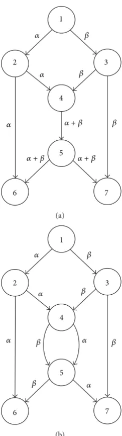
Network coding may significantly improve network perfor-mance in terms of network throughput [1,2]. This advantage of network coding is demonstrated inFigure 1(a), where node 1 is the source, nodes 6 and 7 are sinks, and the capacity of every link is just 1 (in this paper, all links are of unit-capacity). If the nodes in the network only forward and replicate the data they receive, then it is easy to see that one sink can only receive 1 unit of data at one time, although the other sink may achieve a rate of 2. However, with network coding allowed, node 4 inFigure 1(a)may combine data from its two incoming links through the “+” operation, and then at both sinks, a rate of 2 can be achieved by using the “−” operation to decode data. Therefore, network coding increases the total rate of information flow through the same network from 3 to 4, which is obviously a significant improvement. Although network coding is usually allowed at all nodes in most relevant literature, an interesting observation is that a

given target rate can often be achieved by conducting network coding at only a relatively small proportion of the nodes [2]. For instance, in the network given byFigure 1(b), network coding at both node 4 and node 5 will make no difference in terms of the achieved rate at the sinks. In other words, network coding is not necessary in the network ofFigure 1(b). Therefore, a question is raised: at which nodes does network coding need to be conducted, or how to make most of network capacity at a minimal cost in terms of network coding resources? To answer this question, a minimal set of nodes needs to be found for coding, which has been proved to be an NP-hard problem [3].

In this paper, the above problem of minimizing net-work coding resources is referred to as the netnet-work coding problem (NCP). To address this problem, researchers have already attempted many different methods such as minimal approaches [4, 5], linear programming methods [6], and genetic algorithms (GAs) [2, 7–10]. These methods were all reported to be effective to minimize network coding Volume 2014, Article ID 268152, 23 pages

1

2 3

4

5

6 7

𝛼

𝛼

𝛼

𝛽

𝛽

𝛽

𝛼 + 𝛽 𝛼 + 𝛽 𝛼 + 𝛽

(a)

1

2 3

4

5

6 7

𝛼 𝛼 𝛼

𝛼

𝛼 𝛽 𝛽

𝛽 𝛽

𝛽

(b)

Figure 1: Basic idea of network coding.

resources. In particular, like in the applications to many other NP-hard problems, GAs as large-scale parallel stochastic searching and optimization algorithms have demonstrated good potential in resolving the NCP. However, the poor scal-ability of these reported methods largely hampers their appli-cations in the large-scale NCP. For instance, the approaches in both [4,5] determined the minimal set of nodes for coding by removing links in a greedy fashion. The optimal formulations of the linear programming method in [6] involve a number of variables and constraints that grows exponentially with number of sinks. As a family member of population-based algorithms, GAs are generally very expensive in terms of memory demand and computational time in the case of large-scale problems [11,12]. To address the scalability problem, decentralized and distributed versions of algorithms often need to be developed, such as the GAs reported in [7, 9].

Before such decentralized and distributed algorithms can be applied, a problem partitioning method has to be employed in order to divide a large-scale network into some subgraphs of manageable size. This paper attempts to shed a bit of more light on how to design an effective scalable GA for the NCP.

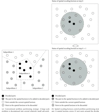
In a conventional problem partitioning method (e.g., see [13, 14]), a large-scale problem is divided into some separate subproblems. Then, each subproblem is resolved in a rather isolated manner. After all subproblems have been resolved independently, their subsolutions are integrated together to form a complete solution to the original large-scale problem. However, even though optimal subsolutions to the subproblems can be found, the integrated complete solution to the original large-scale problem is often not optimal or even good. In other words, optimal subsolutions to the subproblems are often not optimal at all from a global point of view. A main cause of losing the global optimality is the independent/isolated way of resolving each subproblem. In this paper, inspired by the temporal receding horizon control (TRHC) strategy in the area of control engineering [15,16], we propose a novel spatial receding horizon control (SRHC) strategy to partition a large-scale problem. In the SRHC problem partitioning method, a large-scale problem is divided into many subproblems, which compose a problem space; a spatial horizon is then defined which covers some subproblems each time and will recede in the problem space. The spatial horizon is composed of several spatial steps. Each time the spatial horizon recedes by a spatial step. All subproblems covered by a spatial horizon will be optimized as a whole, and only the subsolutions to the subproblems within the first step of the spatial horizon will be saved and fixed, whilst others will be discarded and then recalculated in the next spatial horizon. With the SRHC strategy, a subproblem will be optimized not in an independent/isolated manner, but by making use of its neighboring information in the problem space. Simply speaking, the conventional problem partitioning strategy can be viewed as a one-step-wide SRHC, whilst the new method proposed here is a generalized𝑁 -step-wide SRHC. Obviously, by optimizing a subproblem together with its neighboring sub-problems, it is likely to improve the quality of the associated subsolution in terms of global optimality. The solution quality may be further improved by integrating a GA into the SRHC method by setting up a solution pool for the subproblems in those decided spatial steps.

Start point End point

(a) Offline optimization: optimize the whole dynamic process based on the predicted information in advance, and then the solution is implemented no matter what happens

Start point Current timek k + 1 End point

(b) Conventional dynamic optimization: optimize over the period from the current time𝑘to the end of the dynamic process, and then execute the optimal subsolution over the period from𝑘to𝑘 + 1

Start point Current timek k + 1 k + N End point

· · ·

(c) Temporal receding horizon control (TRHC): optimize over the predictive horizon (from the current time𝑘to time𝑘 + 𝑁), and then execute the optimal subsolution over the period from𝑘to𝑘 + 1

Figure 2: Illustration of temporal receding horizon control (TRHC).

algorithm, in order to significantly improve the overall quality of chromosomes. The remainder of this paper will give the details of the proposed SRHC based GA for the NCP.

2. Basic Idea of SRHC

2.1. Temporal Receding Horizon Control (TRHC) for Dynamic

Problems. First of all, a brief review on the conventional

receding horizon control (RHC) strategy in control engi-neering will be very useful. To distinguish from the method proposed in this paper, the conventional RHC in dynamic control problems is hereafter referred to as temporal receding horizon control (TRHC). TRHC, also known as model predictive control, has proved to be a highly effective online optimization strategy in the area of control engineering, and it exhibits many advantages against other control strategies [15, 16]. It is easy for TRHC to handle complex dynamic systems with various constraints. It also naturally exhibits promising robust performance against uncertainties since the online updated information can be sufficiently used to improve the decision. Simply speaking, TRHC is an𝑁 -step-ahead online optimization strategy to deal with dynamic problems. In this framework, decision is made by looking ahead for 𝑁 steps in terms of a given cost/criterion, and the decision is only implemented by one step. Then the implementation result is checked, and a new decision is made by taking updated information into account and looking ahead for another𝑁steps.

Figure 2illustrates the basic idea of TRHC by comparing it with some other optimization strategies in an intuitive way. Apparently the offline optimization strategy, as shown inFigure 2(a), is not suitable for dynamic environments. The conventional dynamic optimization, as shown inFigure 2(b), is often criticized for its poor real-time properties and poor performance under disturbances and/or uncertainties in dynamic environments. As illustrated inFigure 2(c), thanks to the idea of temporal receding horizon, the TRHC strategy provides a possible solution to the problems confronted by

the conventional dynamic optimization strategy. A properly chosen temporal receding horizon can effectively filter out most unreliable information and reduce the scale of problem. The latter is especially important for complex systems and time-consuming algorithms to satisfy the time limit on the online optimization process. TRHC has now been widely accepted in the area of control engineering [15,16]. Attention has also been paid to applications of TRHC to areas like man-agement and operations research [17–19]. Particularly, the TRHC strategy has recently been reported to be successfully integrated into population-based algorithms to tackle various dynamic NP-hard optimization problems [20–22].

2.2. Spatial Receding Horizon Control (SRHC) for Static

Problems. Inspired by the fact that the success of the TRHC

strategy largely results from decomposing a complex dynamic process into a serial of temporally associated subprocesses, here we are thinking of how to extend the basic idea of TRHC in order to decompose a large-scale static problem into a serial of associated subproblems (please note that con-ventional partitioning methods decompose a static problem into a set of separated subproblems). Then in what terms could subproblems be associated in static environments? Basically, we need to create a problem-specific artificial space, project into the space all parts that compose a solution to the original static problem and then design a spatial horizon which recedes in the space. As the spatial horizon recedes out, the value/status of each part will be optimized along together with all other parts that are within the current horizon scope. Once the values/statuses of all parts are optimized, a final solution to the original static problem is determined. Now, one can see that subproblems will be spatially associated in the artificial space. Therefore, hereafter, we call our new strategy for decomposing static problems as spatial receding horizon control (SRHC).

After an artificial space is designed and all parts that compose a solution are projected into the space, it is crucial to design a spatial horizon receding process to decompose the original static problem into a serial of spatially associated subproblems. A basic spatial horizon receding process can be described as follows. Suppose a solution to a large-scale static problem is composed of 𝑀 local parts. The SRHC strategy makes use of spatial structure (where positions indicate strength of influence between parts of a solution) to move from purely local, part-by-part, optimization to using information from the neighbouring, subglobal context. An optimization algorithm is applied𝑀times to determine the

𝑀parts in a solution. Starting with a specified part, the algo-rithm calculates at each time step the𝑁new parts (usually

𝑁 ≪ 𝑀), which are the most associated with thedecided

Decided parts

Parts outside the current spatial horizon

The part in the spatial horizon to be added to decided parts

Parts in the spatial horizon to be discarded Subproblem 2

Subproblem 1

Subproblem 3 Subproblem 4

(a) Conventional problem partitioning strategy: A large-scale problem is decomposed into several relatively small sub-prob-lems, each sub-problem is resolved in an isolated/independent manner, and then the solutions to all sub-problems are combined together to generate a final solution to the original large-scale problem

Status of spatial receding horizon at stepk

Status of spatial receding horizon at stepk + 1

Decided parts

Parts outside the current spatial horizon

The part in the spatial horizon to be added to decided parts

Parts in the spatial horizon to be discarded

(b) Spatial receding horizon control problem partitioning strat-egy: A spatial horizon covers𝑁new parts around the decided parts. The new parts in the horizon will be calculated in the current run of optimization algorithm. Only the part which is the most associated with the decided parts will be added to update the decided parts, and the other (𝑁 − 1) parts will be discarded. The spatial horizon then recedes for the next run of optimization algorithm

Figure 3: Illustration of Spatial Receding Horizon Control (SRHC).

Existing problem-partitioning methods may be considered as a one-step-wide SRHC strategy; that is, each part of a solution is determined in an isolated manner; for example, see [13]. In the generalized𝑁-step-wide SRHC strategy, each part is calculated by referring to its most relevant surrounding parts. In other words, subglobal information is used in the determination of a local part. The extra information

considered by the𝑁-step-wide SRHC strategy can improve the quality of each part and that of the global solution.

algorithms in dynamic environments [20–22], we will also make an attempt to investigate whether integrating SRHC into GAs can deliver a powerful algorithm to resolve the static large-scale NCP.

2.3. SRHC and GA: A Perfect Match. Like the TRHC scheme

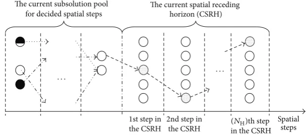
having an online optimizer, the proposed SRHC also needs to run optimization repeatedly as the spatial horizon recedes step by step. General speaking, any optimization algorithm, deterministic or population-based, can be used by the SRHC strategy as long as it suits the concerned problem. However, in this study, we choose GA, because the SRHC strategy and population-based algorithms like GAs are a naturally perfect match to resolve large-scale static problems. On one side, population-based algorithms are very costly in terms of computational time and resources [23, 24]. Such com-putational costs often soar up exponentially as the problem scale increases. Therefore, an effective problem decomposing method like the proposed SRHC is crucial for a population-based algorithm to apply to large-scale problems. On the other side, like all other problem partitioning methods, losing global optimality or having shortsighted performance is still an issue the proposed SRHC has to address. If an algorithm, such as a deterministic algorithm, only outputs a single solution, then due to the receding horizon, the subsolutions for decided spatial steps will be uniquely determined and have no chance to change in future runs, as illustrated in

Figure 4(a). The uniqueness of the subsolutions for decided spatial steps is a major cause of losing global optimality, because an optimal subsolution calculated within a spatial receding horizon may not be optimal or even good at all from a global point of view. If a population-based algorithm is employed, then the optimization within a spatial receding horizon will generate a population of solutions. Some top solutions in the population may usually have different sub-solutions for decided spatial steps. A subsolution pool for decided spatial steps can then be set up according to such top solutions in the population. In the optimization of next spatial receding horizon, it needs not only to calculate those subsolutions covered by the new spatial receding horizon, but also to choose subsolutions from the pool for decided spatial steps. This is illustrated inFigure 4(b). It should be noted that the subsolution pool for decided spatial steps not only records independent subsolutions for each decided spatial step, but more importantly, also records the combination relationships between them as in the associated top solutions. Regarding the decided spatial steps in the new run of optimization, it actually only needs to choose a combination relationship saved in the pool. This can significantly reduce the search space for decided spatial steps. For instance, inFigure 4(b), the independent subsolutions saved in the pool may have at least 6 combinations for decided spatial steps, but the choice needs to be made between only 3 combinations as given by the previous run of optimization. At the same time, the global performance can be effectively improved, because some flexibility in the subsolutions for decided spatial steps is introduced by the pool referring to some top solutions of the previous spatial receding horizon. Therefore,

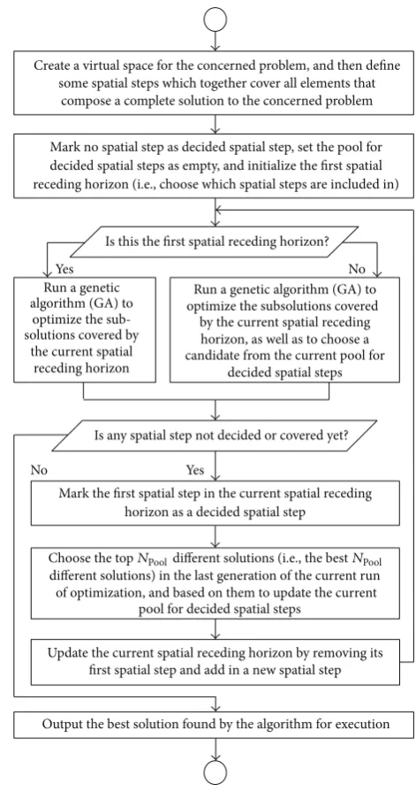
a population-based algorithm like GA can help to improve the global performance of the SRHC.Figure 5summarizes the combination of the SRHC scheme with GA as a flowchart.

3. Modeling NCP Based on SRHC

3.1. Conventional Model of NCP. Suppose a network, denoted

as𝐺{𝑉, 𝐸}hereafter, where𝑉and𝐸are sets of vertices and

edges, that is, nodes and unit-capacity links in this paper, respectively, has𝑛_𝑛nodes and𝑛_𝑙links. This paper considers only the one-source-multisink SNCP, so, all data originate from a certain node and need to go to some other nodes. For the sake of simplicity, but without losing generality, in this paper it is assumed that the source is always node 1 in the network. Let𝑛_𝑑 be the number of signals originating from the source,𝑛_𝑠be the number of sinks in𝐺{𝑉, 𝐸}, and𝑅Targetbe the target rate which is expected to be achieved at every sink. Basically, a network protocol and coding scheme define how each node in the network forwards, replicate, and/or encodes data. For instance, assuming that node𝑖has𝑛_In(𝑖)incoming links and 𝑛Out(𝑖) outgoing links and the signal on the jth incoming link is𝑠_In(𝑖, 𝑗), then a network protocol and coding scheme can be viewed as a mapping process to generate the signals on outgoing links; that is,𝑠Out(𝑖, 𝑗),𝑖 = 1, . . . , 𝑛_𝑛, 𝑗 =

1, . . . , 𝑛Out(𝑖). Mathematically, a network protocol and coding

scheme can be denoted as

𝑀NPCS: {𝐺 (𝑛_𝑛, 𝑛_𝑙) , 𝑠_In(1, ℎ)} 󳨀→ 𝑠Out(𝑖, 𝑗)

ℎ = 1, . . . , 𝑛_𝑑, 𝑖 = 1, . . . , 𝑛_𝑛, 𝑗 = 1, . . . , 𝑛Out(𝑖) . (1)

The most widely used coding operation is linear network coding, which can be mathematically formulated as follows for an outgoing link:

𝑠Out(𝑖, 𝑗) =𝑛In(𝑖)∑

ℎ=1

𝑤 (𝑖, 𝑗, ℎ) 𝑠_In(𝑖, ℎ) ,

𝑖 = 1, . . . , 𝑛𝑛, 𝑗 = 1, . . . , 𝑛Out(𝑖) ,

(2)

where 𝑤(𝑖, 𝑗, ℎ), ℎ = 1, . . . , 𝑛_In(𝑖) are weights determining how to combine the 𝑛_In(𝑖) incoming signals of node 𝑖 to generate a signal for the jth outgoing link of node 𝑖. In theory,𝑤(𝑖, 𝑗, ℎ)may be continuous, but as proved by [25,26], sufficient finite discrete values for𝑤(𝑖, 𝑗, ℎ)can guarantee that the maximum possible throughput is achieved. Therefore, in this paper,𝑤(𝑖, 𝑗, ℎ)will choose its value from a finite setΘ_𝑊. Assuming thatΘ_𝑊has𝑁_𝑊≥ 2discrete values, then the field size for network coding is𝑁_𝑊in this study. A linear coding scheme is actually defined by a set of𝑤(𝑖, 𝑗, ℎ), in other words, all that is required in order to design a linear coding scheme is the appropriate choice of𝑤(𝑖, 𝑗, ℎ). Apparently, a network protocol and coding scheme is actually determined by the set

of𝑤(𝑖, 𝑗, ℎ). For a given network protocol and coding scheme,

suppose the numbers of coding nodes and links are𝑁CNand 𝑁CL, respectively, and the actually achieved rate at sink𝑖is

· · ·

Time Current

timek k + 1 k − 1

· · ·

1

A candidate subsolution for a time instant (different time instant may have different candidate subsolutions to choose from)

Unique combination relationship determined by the subsolutions for the past time instants

Undecided combination relationship within the current temporal receding horizon

A decided subsolution for a past time instant, which is unchangeable in any future run of optimization

A subsolution newly calculated for a time instant within the current temporal receding horizon

Subsolutions for the past time instants

The current temporal receding horizon

k + NH− 1

(a) In temporal receding horizon control, no matter what kind of method, deterministic method or population-based algorithm, is used as the online optimizer, the sub-solutions for the past time instants will have been uniquely decided and executed, and the sub-solutions for the future time instants will be optimized only based on the unchangeable consequence of the past sub-solutions. Therefore, short-sighted behaviours are common in temporal receding horizon control, because the unchangeable past sub-solutions might not be optimal or even good in terms of the performance over the entire time scope. A combination of spatial receding horizon control and deterministic method has the same solution pattern (except the time axis is replaced by a spatial axis)

The current subsolution pool for decided spatial steps

Fixed combination relationships given by candidates in the current subsolution pool

for decided spatial steps

Undecided combination relationship within the CSRH, which needs to be calculated in the current run of optimization

· · · ·

A candidate subsolution for a spatial step (different spatial step may have different candidate subsolutions to choose from)

A subsolution for a decided spatial step, which may change depending on which candidate in the current pool for decided spatial steps is chosen

A subsolution newly calculated for a spatial step within the CSRH The current spatial receding

horizon (CSRH)

Spatial

steps

1st step in the CSRH

2nd step in

the CSRH _{in the CSRH}

(NH)th step

(b) In spatial receding horizon control combined with population-based algorithm, the sub-solutions for decided spatial steps are not fixed or executed. Based on some top different solutions (e.g., the best 10 different solutions) calculated in the last rune of optimization, a sub-solution pool is set up for decided spatial steps. Different candidates in the pool may have different sub-solutions for a same decided spatial step. Therefore, in the current run of optimization, besides calculating the sub-solutions for the spatial steps within the current spatial receding horizon (CSRH), it also needs, for the sake of optimality, to choose a candidate from the pool for those decided spatial steps

With the above preparation, the NCP in this paper is formulated as the following maximization problem:

max

𝑀NPCS𝑓1=𝑤max(𝑖,𝑗,ℎ)𝑓1,

𝑖 = 1, . . . , 𝑛𝑛, 𝑗 = 1, . . . , 𝑛Out(𝑖) , ℎ = 1, . . . , 𝑛In(𝑖) ,

(3)

where

𝑓₁=

{ { { { { { { { { { { { { { { { { { { { { { { { { { { { { { { { { { { { { { {

𝛼₁min(𝑅 (𝑖)) + 𝛼₂ave(𝑅 (𝑖))

+ 𝛼3

(𝑁CL+ 1)

+ 𝛼4

(𝑁CN+ 1), min(𝑅 (𝑖)) < 𝑅Target,

𝛼₁min(𝑅 (𝑖)) + 𝛼₂ave(𝑅 (𝑖))

+ 𝛼5

(𝑁CL+ 1)

+ 𝛼6

(𝑁CN+ 1)

, min(𝑅 (𝑖)) ≥ 𝑅Target,

𝑖 = 1, . . . , 𝑛s

(4)

𝛼_𝑘, 𝑘 = 1, . . . 6, are weights, and

min(𝛼₁, 𝛼₂) >max(𝛼₃, 𝛼₄) ,

min(𝛼₅, 𝛼₆) ≫max(𝛼₁, 𝛼₂) ,

(5)

subject to𝐺(𝑛_𝑛, 𝑛_𝑙). Clearly, this maximization problem aims to find a network protocol and coding scheme to maximize𝑓₁ defined by (4) and (5). From the above objective function, one can see that the NCP will firstly try to maximize the overall actually achieved rate, and once the target rate is achieved, the focus of the optimization will switch to minimizing the network coding resources. The term “min(𝑅(𝑖))” and term “ave(𝑅(𝑖))” in (4) can be used to assess the actually achieved rate. Basically, a larger term value for “ave(𝑅(𝑖))” is desirable.𝑅(𝑖)should be optimized as evenly as possible; that is, increasing the rate at some sinks by largely sacrificing the rate at other sinks should be avoided. This can be reflected by the term value for “min(𝑅(𝑖));” that is, the larger the value is, the more evenly𝑅(𝑖)is optimized. At the same time, as reflected by the term “1/(𝑁CL+ 1)” and the term “1/(𝑁CN+

1),” the network coding resources should be minimized, particularly when the target rate can be achieved, that is, when min(𝑅(𝑖)) ≥ 𝑅Target.

3.2. SRHC Based Model for NCP. To design an SRHC

based model for the NCP, firstly we need to create an artificial space, then to project all network nodes into the space, then to design a spatial horizon receding pro-cess, and at last to reformulate the maximization problem given by (3) to (5) in order to make it fit in the SRHC framework.

Usually, a network where coding needs to be performed already defines its own space (real or virtual) and may have its

Mark the first spatial step in the current spatial receding

horizon as a decided spatial step

Update the current spatial receding horizon by removing its first spatial step and add in a new spatial step

Output the best solution found by the algorithm for execution

Choose the topNPooldifferent solutions (i.e., the bestNPool

different solutions) in the last generation of the current run of optimization, and based on them to update the current

pool for decided spatial steps

Create a virtual space for the concerned problem, and then define

some spatial steps which together cover all elements that compose a complete solution to the concerned problem

Mark no spatial step as decided spatial step, set the pool for decided spatial steps as empty, and initialize the first spatial receding horizon (i.e., choose which spatial steps are included in)

Yes No

Is this the first spatial receding horizon?

Run a genetic algorithm (GA) to

optimize the sub-solutions covered by

the current spatial receding horizon

Is any spatial step not decided or covered yet?

Run a genetic algorithm (GA) to optimize the subsolutions covered by the current spatial receding horizon, as well as to choose a candidate from the current pool for

decided spatial steps

No Yes

Figure 5: Flowchart of SRHC with GA as online optimizer.

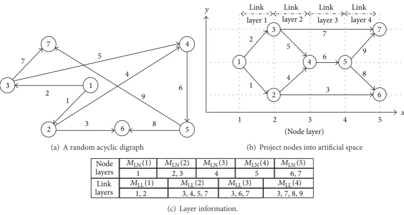
nodes distributed in the space in a rather random manner, but such a space and the distribution of nodes are of little use to the design of artificial space and the projection of nodes in the SRHC model for the NCP. In the SRHC model, we simply use a purely imaginary two-dimensional space and then project network nodes into the space according to the connections between nodes. The projecting procedure is described as follows.

Step 1. Let𝑀LN(𝑖)be the set that records all nodes in the𝑖th

node layer, and𝑀LL(𝑖)records all links in the𝑖th link layer.

Start from the source, that is, node 1. Set node 1 as the only node in𝑀LN(1), and set the end nodes of all outgoing links

of node 1 as the nodes in𝑀LN(2). Then set the current layer 𝑙𝐶= 2. LetΩ𝑁be the set of all nodes that are not included in

7

4

2

5

3

9 1

8 6 3

2 7

1

5 4

6

(a) A random acyclic digraph

4 5

5 9

8

1 1

2

6 1

3 3

4 4

7

2 2

6 5

7 3

Link Link Link Link

layer 1 layer 2 layer 3 layer 4

x

(Node layer)

y

(b) Project nodes into artificial space

Node

layers

MLN(1) MLN(2) MLN(3) MLN(4) MLN(5)

1 2,3 4 5 6,7

Link layers

MLL(1) MLL(2) MLL(3) MLL(4)

1,2 3,4,5,7 3,6,7 3,7,8,9

(c) Layer information.

Figure 6: An illustration of node projecting procedure.

Step 2. WhileΩ_𝑁 ̸=Ø, do

Substep 2.1. Put all end nodes of all outgoing links of the nodes

in𝑀LN(𝑙_𝐶)as the nodes in𝑀LN(𝑙_𝐶+ 1).

Substep 2.2. If a node in𝑀LN(𝑙_𝐶+ 1)is already included in

𝑀LN(𝑖), 𝑖 = 1, . . . , 𝑙_𝐶, then remove this node from𝑀LN(𝑖),

and add it toΩ_𝑁.

Substep 2.3. Remove all nodes of𝑀LN(𝑙_𝐶+ 1)fromΩ_𝑁. Let

𝑙_𝐶= 𝑙_𝐶+ 1.

Step 3. Create a two-dimensional space, where the𝑥 axis

is the node layer number, and the 𝑦 axis has no specific meaning. Then project all nodes into the space according to

𝑀LN. For instance, suppose a node belongs to𝑀LN(𝑖). Then

the𝑥coordinate of this node is𝑖. The𝑦coordinate of this node can be random, but for distinguishing purposes, the nodes in the same layer should be assigned with different values of𝑦.

Step 4. For a link, suppose its starting node is within𝑀LN(𝑖)

and its end node within𝑀LN(𝑖),𝑗 > 𝑖. Then add this link to

𝑀LL(𝑖), . . . , 𝑀LL(𝑗 − 1).

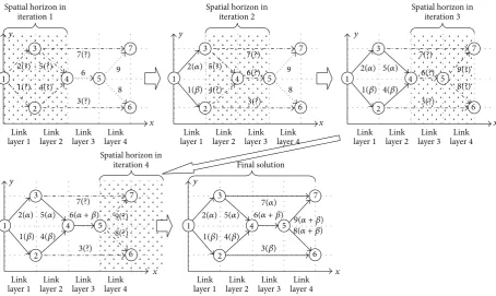
Figure 6gives a simple illustration about the above node projecting procedure. The information of node layers and link layers is crucial not only to define the spatial horizon, but also to design the spatial horizon receding process for the NCP. As illustrated inFigure 7, the spatial horizon for the NCP is defined based on link layers. In each iteration of optimization, the spatial horizon covers some successive link layers; for example, in the case ofFigure 7, the spatial horizon spans over two successive link layers. In an iteration of optimization, only those links that are covered by the current spatial horizon will be optimized. The spatial horizon

recedes for one link layer each time along the𝑥axis in the artificial space. In the new iteration of optimization, those links that have been optimized in the previous iteration of optimization and get out of the current spatial horizon due to the horizon receding process will be fixed as decided links, whilst those links that have been optimized in the previous iteration of optimization but are still within the current spatial horizon will be optimized again along with the links that are newly covered by the spatial horizon. This process continues until all links become decided links. The details of the spatial horizon receding process are given as follows.

Step 1. Set up𝑁_𝐻, the length of the spatial horizon. LetΩ_𝑆

be the set of sinks,ΩDL = Ø the set of decided links, and

ΩUL = {𝑀LL(1), . . . , 𝑀LL(𝑁LL)}the undecided links, where

𝑁LLis the number of total link layers. Let𝑘 = 1.

Step 2. WhileΩUL ̸=Ø, do

Substep 2.1. Set the current spatial horizon as Ω_𝐻(𝑘) =

{𝑀LL(𝑘), . . . , 𝑀LL(𝑘 + 𝑁_𝐻 − 1)}. It should be noted that

𝑀LL(𝑖) =Ø for𝑖 > 𝑁LL.

Substep 2.2. Let 𝑊(𝑘) be the weights for the links in

Ω_𝐻(𝑘), 𝑀EN(𝑘 + 𝑁_𝐻− 1)the set of all end nodes of the links

in𝑀LL(𝑘 + 𝑁_𝐻− 1), and𝑁CL(𝑘)and𝑁CN(𝑘)are the current

numbers of coding links and coding nodes, respectively. Then calculate the following maximization problem:

max

𝑊(𝑘)𝑓2(𝑘) , (6)

subject to the signals onΩDL, where𝑓₂(𝑘)is a new objective function defined as follows:

𝑓₂(𝑘) = 𝛽₁𝑓NT(𝑀EN(𝑘 + 𝑁𝐻− 1))

Link layer1 Link layer2 Link layer3 Link layer4 Link layer1 Link layer2 Link layer3 Link layer4 Link layer1 Link layer2 Link layer3 Link layer4 Link layer1 Link layer2 Link layer3 Link layer4 Link layer1 Link layer2 Link layer3 Link layer4

Spatial horizon in iteration4

Spatial horizon in iteration1

Spatial horizon in iteration3

Spatial horizon in iteration2

Final solution

A decided link

A link under optimization

An undecided link out of the current spatial horizon

x

x x x

x y

y y y

y 1 2 3 4 5 6 6 7 8 9 1 2 3 4 5 6 7 8 9 1 2 3 4 5 6 7 2(?) 1(?) 5(?) 4(?) 3(?) 7(?) 5(?) 4(?)

3(?) 3(?)

8(?)

9(?)

6(?) 6(?)

7(?) 7(?)

1(𝛽) 1(𝛽) 4(𝛽)

2(𝛼)

2(𝛼) ₅(𝛼)

6(𝛼 + 𝛽) 1 2 3 4 5 6 7 3(?) 8(?) 9(?) 7(?)

1(𝛽) 4(𝛽)

2(𝛼) 5(𝛼)

1 2 3 4 5 6 7

1(𝛽) 4(𝛽)

3(𝛽)

2(𝛼) 5(𝛼) 6(𝛼 + 𝛽)

9(𝛼 + 𝛽)

8(𝛼 + 𝛽)

7(𝛼)

Figure 7: An illustration of spatial horizon receding process.

+ 𝛽₃𝑓SD(𝑀EN(𝑘 + 𝑁𝐻− 1)) +_(𝑁CL𝛽_{(𝑘) + 1)}4

+ 𝛽5

(𝑁CN(𝑘) + 1)+ 𝛽6𝑓TP(𝑘, Ω𝑆) ,

(7)

which will be explained later.

Substep 2.3. Remove𝑀LL(𝑘)fromΩULtoΩDL; that is,ΩUL=

ΩUL− 𝑀LL(𝑘)andΩDL= ΩDL+ 𝑀LL(𝑘). Let𝑘 = 𝑘 + 1.

In the above spatial horizon receding process, a new maximization problem as defined by (6) and (7) needs to be resolved during each iteration of optimization. In the new objective function𝑓₂(𝑘), the term𝑓NT(𝑀EN(𝑘 + 𝑁_𝐻− 1)) is a function that calculates the network throughput at all nodes in𝑀EN(𝑘 + 𝑁_𝐻 − 1), the term𝑓MR(𝑀EN(𝑘 + 𝑁_𝐻−

1))is a function that calculates the minimal rate over the nodes in𝑀EN(𝑘 + 𝑁_𝐻 − 1), the term𝑓SD(𝑀EN(𝑘 + 𝑁_𝐻 −

1)) is a function that assesses how much the signals on

𝑀EN(𝑘 + 𝑁_𝐻 − 1) are diversified, the term 𝑓TP(𝑘, Ω_𝑆) is a

terminal penalty which assesses the impact of the current stage solution on the network throughput at the sinks, and

𝛽₁to𝛽₆are weights to combine different terms. Apparently

𝑓₂(𝑘) is quite different from the objective function of the conventional NCP model, that is,𝑓₁as defined in (4), mainly because of two new terms: 𝑓SD(𝑀EN(𝑘 + 𝑁_𝐻 − 1)) and

𝑓TP(𝑘, Ω𝑆). The reason for introducing𝑓SD(𝑀EN(𝑘+𝑁𝐻−1))

is illustrated inFigure 8, where one can see that, assuming all other terms in𝑓₂(𝑘)are the same, Figure 8(a)is better thanFigure 8(b)because the signals on𝑀EN(𝑘 + 𝑁𝐻− 1)are

better diversified, which means the downstream nodes will have more choices. The introduction of𝑓TP(𝑘, Ω𝑆)is in line

with the common practice of TRHC in the area of control engineering, which aims to minimize shortsighted behaviors, such as getting trapped in local optima and generating unstable/unconverged solutions, due to the fact that not all information is covered by the receding horizon. Before running the SRHC model, we need to count the number of downstream sinks for every node in the network. Then we can roughly assess the final impact of the signals received by a node. Basically, a node with more downstream sinks deserves a higher priority to receive more signals, just likeFigure 9

illustrates.

The absolute value of different term in𝐽₂may vary in quite different range; for example,𝑓NTmay be over 1000 whilst𝑓MR

may be smaller than 10. This means the absolute values of different terms in𝐽₂are usually incomparable, and then they cannot be directly combined by𝐽₂. Therefore we need to unify the terms of𝐽₂; in other words, we have to use the relative value of each term, as defined by the following:

𝑓3(𝑘) = 𝛽1𝑓NT(𝑀EN(𝑘 + 𝑁𝐻− 1))

· · ·

a b c

a _b c a

b c

d

MEN(k + NH− 1)

Source

(a) A case where signals are less diversified

· · ·

a b c

a _b c b

c d

d

MEN(k + NH− 1)

Source

(b) A case where signals are more diversified

Figure 8: An illustration of signal diversification.

a

b a a b c

Downstream sinks of noden

Downstream sinks of nodem

n m

· · · ·

· · · ·

· · · · · ·

· · · · MEN(k + NH− 1)

(a) A case where terminal penalty is larger

a

b c b c b

Downstream sinks of noden

Downstream sinks of nodem

n m

· · · · MEN(k + NH− 1)

· · · ·

· · ·

(b) A case where terminal penalty is smaller

Figure 9: An illustration of terminal penalty.

+ 𝛽₃𝑓SD(𝑀EN(𝑘 + 𝑁𝐻− 1)) +

𝛽₄

(𝑁CL(𝑘) + 1)

+ 𝛽5

(𝑁CN(𝑘) + 1)

+ 𝛽₆𝑓TP(𝑘, Ω𝑆) ,

(8)

𝑓NT(𝑀EN(𝑘 + 𝑁𝐻− 1)) =

𝑓NT(𝑀EN(𝑘 + 𝑁𝐻− 1))

𝐹NT(𝑀EN(𝑘 + 𝑁𝐻− 1)), (9)

𝑓MR(𝑀EN(𝑘 + 𝑁𝐻− 1)) =

𝑓MR(𝑀EN(𝑘 + 𝑁𝐻− 1))

𝐹MR(𝑀EN(𝑘 + 𝑁_𝐻− 1)),

(10)

𝑓SD(𝑀𝐸𝑁(𝑘 + 𝑁𝐻− 1)) =

𝑓SD(𝑀EN(𝑘 + 𝑁𝐻− 1))

𝐹𝑆𝐷(𝑀𝐸𝑁(𝑘 + 𝑁𝐻− 1)), (11)

𝑓TP(𝑘, Ω𝑆) =

𝑓TP(𝑘, Ω𝑆)

𝐹TP(𝑘, Ω_𝑆), (12)

1 10 19

2 11 20

3 12 21

4 ₁₃ 22

5 14 23

6 15 24

7 16 25

8 17 26

9 18 0 0

x1 _x

2

x3

x1/2

x2/2

x3/2

x1

x2

x3

x1/2 + x2/2

x1+ x2/2

x1/2 + x2

x1+ x2

x1+ x3

x2+ x3

x1/2 + x3/2

x2/2 + x3/2

x1+ x3/2

x2+ x3/2

x1/2 + x3

x2/2 + x3

x1/2 + x2/2 + x3/2

x1/2 + x2/2 + x3

x1+ x2/2 + x3/2

x1+ x2/2 + x3

x1/2 + x2+ x3/2

x1/2 + x2+ x3

x1+ x2+ x3/2

x1+ x2+ x3

k y k y k y

y =∑wixi

wherewi= 0, 1/2, 1,

andi = 1, 2, 3.

Figure 10: An illustration of definition of signal combinations.

4. SRHC Based GA for NCP

The design of GAs usually includes choosing an appropri-ate chromosome structure, developing effective evolution-ary operators, introducing useful problem-specific heuristic rules, and adjusting algorithm-related parameters. This sec-tion will explain the first three aspects, and the last aspect will be discussed in the experiment section. Here we will firstly spend three subsections to describe some useful GA-related designs reported in [10]. Then some SRHC-related modifications to the GA designs will be discussed in order to properly integrate the GA into the SRHC method for the NCP.

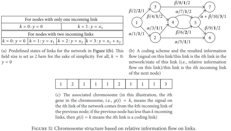
4.1. Chromosome Structure. The chromosome structures of

the GAs in [2,7,8] are based on the use of a binary matrix to record the active states of links, and such structures make it easy to apply graph theoretic methods to ascertain whether the target rate is or is not achievable by a given chromosome. A chromosome in [2, 7, 8] does not have full information concerning a specific network protocol and coding scheme and may associate with different specific network protocols and coding schemes. Although this means to some extent random linear coding can be employed, it may be difficult to determine the exact information flow on links. The lack of exact information flow on links will make it difficult not only to calculate the actually achieved rate at sinks, but also to integrate useful NCP-specific heuristic rules into the algorithms. Therefore, in this paper we construct chromosomes based on a permutation representation, in order to record exact information flow on links.

A permutation representation is often used when GAs are being applied to combinatorial problems (actually, the NCP is a combinatorial problem), because it can usually construct chromosomes straightforwardly based on their physical meanings. However, such a representation is often confronted by feasibility problems; that is, a chromosome may become infeasible in terms of its physical meaning dur-ing evolutionary operations. Sometimes some evolutionary operators have to be modified significantly or even discarded

in order to resolve such problems. For the NCP, a straight-forward permutation representation is to use the absolute information flow on links to construct chromosomes, but this representation will cause serious feasibility problems during evolutionary operations, because the set of feasible signals from which a link can choose cannot be predetermined and varies over time according to the signals on other links. This means that any change in the signal on a link caused by evolutionary operations could make the unchanged signals on some other links infeasible.

Fortunately, the permutation representation in [10] is free of feasibility problems without sacrificing any of the merits of permutation representations. Instead of the absolute information flow on links, a chromosome in [10] records the relative information flow, that is, an integer𝑘, whose meaning is a certain predefined combination of signals on incoming links of a node. For instance,Figure 10shows an illustration of how to predefine𝑘. InFigure 10, a table is set up to define all possible signal combinations at a node with three incoming links, and the field size is𝑁_𝑊 = 3. A different number of incoming links require a different predefined table for𝑘, as illustrated inFigure 11.

Let ℎ𝑒𝑎𝑑(𝑖) denote the serial number of the starting

node of link 𝑖. It is assumed that the source has as many incoming links as there are signals to be sent, and each signal is associated with one and only one of such assumed links. Let gene𝑖, that is,𝑔(𝑖), be associated with link𝑖.Then𝑔(𝑖) =

𝑘, 𝑘 = 0, 1, . . . , 𝑁_𝑊𝑛In(ℎ𝑒𝑎𝑑(𝑖)), where𝑛_In(ℎ𝑒𝑎𝑑(𝑖))is the number

of incoming links from nodeℎ𝑒𝑎𝑑(𝑖). In other words, for an outgoing link, for example, link 𝑖, the number of possible combinations (including no coding) is𝑁_𝑊𝑛In(ℎ𝑒𝑎𝑑(𝑖)). The exact combination that a value of𝑘stands for needs be predefined. Hereafter, the value of𝑔(𝑖)is called thestateof link𝑖. Then the set of possiblestatesfor link𝑖is

Θ_𝑆(𝑖) = {0, 1, . . . , 𝑁𝑛In(ℎ𝑒𝑎𝑑(𝑖))

𝑊 } . (13)

Therefore, the size of the solution space of the GA is

𝑛SP=∏𝑛𝑙

𝑖=1

For nodes with only one incoming link

For nodes with two incoming links

k = 0: y = 0

k = 0: y = 0

k = 1: y = x1

k = 1: y = x1 k = 2: y = x2 k = 3: y = x1+ x2

(a) Predefined states of links for the network inFigure 1(b). This field size is set as 2 here for the sake of simplicity. For all,𝑘 = 0:

𝑦 = 0

𝛼/1/1/1

𝛽/2/2/1

𝛼/3/1/1

𝛼/5/1/1 𝛽/4/1/2

𝛽/8/1/2

𝛼/7/1/2

𝛽/9/1/2 𝛼 + 𝛽/10/3/1

𝛽/6/2/1 1

2 3

4 5

6 7

(b) A coding scheme and the resulted information flow (signal on this link/this link is theith link in the network/state of this link (i.e., relative information flow on this link)/this link is theith incoming link of the next node)

1 2 1 1 1 2 1 1 1 3

(c) The associated chromosome (in this illustration, theith gene in the chromosome, i.e.,𝑔(𝑖) = 𝑘, means the signal on theith link of the network comes from thekth incoming link of the previous node; if the previous node has less thankincoming links, then𝑔(𝑖) = 𝑘means theith link is a coding link)

Figure 11: Chromosome structure based on relative information flow on links.

Unlike the absolute information flow on the links,Θ_𝑆(𝑖) only depends on the network topology and the number of signals that are to be sent, which are both fixed during a GA run. Therefore, as long as 𝑔(𝑖) remains within Θ_𝑆(𝑖) during the evolutionary operation, there will be no feasibility problem. As will be discussed in the following subsection, this condition is very easily fulfilled. On the other hand, the absolute information flow on links can be derived in a straightforward way from a chromosome of the new GA. The simple illustration inFigure 11indicates how to use relative information flow on links to construct a chromosome.

The chromosome described above is a vector with a size of𝑛_𝑙. One may also use a𝑛_𝑙×max(𝑛_In(𝑖))matrix to record, for each link, the weights applied to its incoming links. Such a matrix representation will need no predefined tables. In this study, we choose the vector representation because (i) it has a lower memory demand, particularly in the case of large-scale networks,and (ii) it is more efficient in terms of algorithm execution (the matrix representation requires to generate𝑛_In(ℎ𝑒𝑎𝑑(𝑖))random numbers to determine the relative information flow on link 𝑖, whilst the vector rep-resentation needs only one random number). However, for networks where a node may have many incoming links, the predefined tables for the vector representation will become enormously huge if the field size is also large. For instance, assuming max(𝑛_In(𝑖)) = 10and𝑁_𝑊 = 10, then the largest predefined table will have 1010entries for𝑦. In this case, we can transform the network into an equivalent network which has a relatively small max(𝑛_In(𝑖)). Actually, we can always transform a network into a new one with max(𝑛_In(𝑖)) = 2, as illustrated in Figure 12, and then even if 𝑁_𝑊 = 100, the largest predefined table only needs1002 = 104 entries for𝑦. The transformed network will have more links than the original network, which means, according to (14), that the entire search space will increase, which will particularly become of concern in the case of large-scale networks if no problem partitioning method is used. Fortunately, with the

x1 _x2 x3 x1 x2 x3

y1 y2 y3 y1 y2 y3

Figure 12: Transform a network into a new network with max(𝑛_In(𝑖)) = 2.

proposed SRHC method to decompose large-scale networks, the search space during a spatial receding horizon can easily be restricted to a manageable size, no matter how large the original network scale is.

It should be noted that the search space given by (13) and (14) is much larger than those in previous studies. For instance, the search space size for link𝑖is2𝑛In(ℎ𝑒𝑎𝑑(𝑖)) _{in [2],}

4.2. Evolutionary Operators. The mutation operator in this paper is designed as follows. A chromosome is chosen for mutation with probability𝑝_𝑚. Then a gene associated with a potential coding link needs to be chosen randomly. Suppose the𝑖th gene, that is,𝑔(𝑖), is chosen, whose associated link is the𝑖th link in the network. Then the set of possible states for link𝑖is given byΘ_𝑆(𝑖) as defined in (13). Mutation will randomly choose a value from the setΘ_𝑆(𝑖) − {𝑔(𝑖)}and then reset𝑔(𝑖)to the new value. SinceΘ_𝑆(𝑖)only depends on the network topology, the above mutation operation is free of feasibility problems.

This paper adopts uniform crossover, which is highly efficient in not only identifying, inheriting, and protecting common genes, but also in terms of recombining noncom-mon genes [17,27]. Simply speaking, in uniform crossover, each gene of an offspring chromosome inherits the associated gene from its two parent chromosomes with a 50% chance. Thanks to the permutation representation, the𝑖th genes of all chromosomes share the same set of possible states for link

𝑖, and, therefore, uniform crossover will cause no feasibility problems. Regarding the choice of two parent chromosomes, any chromosome in an old generation may be chosen as the first parent chromosome at a fixed probability of𝑝_𝑐, and then a different chromosome may be chosen as the second parent chromosome at a probability proportional to its fitness. In this way, every chromosome stands the same chance to become the first parent, while a fitter chromosome stands a better chance to cross over with most other chromosomes.

4.3. Heuristic Rules. It is well known that heuristic rules,

particularly problem-specific rules, often play an important role in successful applications of GAs. What kinds of rules to introduce and how to integrate them into algorithms effectively are challenging tasks and usually need to be taken into account in the GA design stage. The permutation representation discussed inSection 4.1makes it very easy to integrate the following NCP-specific rules.

Rule 1. All evolutionary operations only apply to potential

coding nodes and links.

Rule 2. When initializing the first generation, a certain

proportion of chromosomes will allow coding on all potential coding nodes, and for a potential coding node which has multiple outgoing links, choose at least one link randomly as a coding link. This rule can help to find a solution to achieve the target rate, if it is achievable, at all sinks.

Rule 3. Furthermore, in the initialization of the first

gen-eration, another proportion of chromosomes will allow no coding at all. This rule can help to explore the possibility of maximizing the rate actually achieved at the minimum cost of resources.

Rule 4. In either initialization or evolutionary operations, the

states of incoming links of a potential coding node should be determined in such a way that the node will receive as many different signals as possible. In other words, the signals to a potential coding node should be diversified as much

as possible. This rule will allow as many choices as possible for network protocols and coding schemes and therefore can help to diversify a generation. It should be noted that it is the proposed permutation representation that makes it possible to integrate this rule into the algorithm, because the information flow on links associated with a chromosome can be easily checked out to see whether the signals to potential coding nodes are effectively diversified.

Rule 5. For a potential coding node with multiple outgoing

links, there should be a high probability that the outgoing links have different states. This rule also takes advantage of the proposed permutation representation and can help to diversify a generation.

It should be noted that Rules4and5cannot be used by the methods reported in [2,7–9], because the application of Rules

4and5demands the availability of the exact information flow on links, which is guaranteed by the chromosome structure adopted in this paper. As will be revealed by the simulation results, Rules4and5can significantly improve the quality of chromosomes.

4.4. SRHC Related Modifications in GA. In order to properly

integrate the above GA-related designs into the SRHC for the NCP, two modifications are necessary. One is related to the chromosome structure, and the other to the mutation opera-tion. Hereafter for distinguishing purposes, a GA designed according to the above three subsections is referred to as GlobalGA, because no problem partitioning method is used, whilst a GA with the SRHC-related modifications discussed in this subsection is called SRHCGA. The SRHCGA can also be interpreted as the combination of the SRHC with GA, or an SRHC method with GA as optimizer.

As discussed in Section 2, in the SRHCGA, the opti-mization within a spatial receding horizon not only needs to calculate the subsolutions to the subproblems covered by the spatial receding horizon, but also has to choose the subsolutions for the subproblems in decided spatial steps. In the case of applying the SRHCGA to the NCP, besides assigning relative signals to the undecided links covered by the current spatial receding horizon, the optimization within the horizon will also choose a combination of relative signals for all decided links, and all candidate combinations are saved in a pool which is updated as the spatial horizon recedes. To be able to make such a choice for decided links, we need an additional special gene in the chromosome structure to record which candidate combination in the pool is chosen. This can be easily done by modifying the chromosome structure in Section 4.1 as follows. Suppose there are 𝑁SP candidate combinations in the current pool for decided links and 𝑁ULSRHC undecided links in the current spatial receding horizon. Then the modified chromosome structure

has(𝑁ULSRHC+ 1)genes in total. The first gene records which

candidate combination in the pool is chosen for decided links, that is,𝑔(1) = 𝑚, 𝑚 ∈ {1, . . . , 𝑁SP}, means that the mth

candidate combination saved in the pool has been chosen to set up the relative signals on decide links. The following

Link

layer1

Link

layer2

Link

layer3

Link

layer4

Current spatial receding horizon

A decided link

A link under optimization An undecided link out of the current spatial horizon

∙The definition of relative signals is given

in Figure 11(a)

∙In this illustration, it is assumed there are two candidate combinations of relative signals in the pool for the decided links,

1(𝛼 + 𝛽)and link2(𝛽). 4(𝛽)

5(𝛼 + 𝛽) ₉

8

x y

1(𝛽)

2(𝛼 + 𝛽) 6(𝛼 + 2𝛽) 7(𝛼 + 𝛽)

3(𝛽) 1

3

4

7

2 6

5

1(𝛼) and link2(𝛽); combination2: link

that is, link1and link2. Combination1: link

(a) A coding solution under the SRHC

2 1 1 1 3 1

the pool is chosen for the decided links.

assigned to link3to link7, respectively. g(1) records which combination of relative signals in

g(2) tog(6) record which relative signals are

(b) The associated chromosome

Figure 13: An illustration of the modified chromosome structure for SRHC.

the relative signals assigned to the undecided links covered by the spatial horizon, and their definition is exactly the same as described inSection 4.1. All candidate combinations in the pool for decided links are predetermined by the optimization of the previous spatial receding horizon and then are fixed during the optimization of the current spatial horizon. Therefore, the new 𝑔(1) will cause no feasibility problem, just like other genes which record relative signals.

Figure 13gives an illustration of the modified chromosome structure for SRHC.

The second SRHC-related modification is made to the mutation operation given inSection 4.2. Actually, the modifi-cation is minor: the search space for the new𝑔(1)is not given by (13), and𝑔(1)always mutates within{1, . . . , 𝑁SP} − 𝑔(1).

5. Experimental Results

In this section, we will firstly test whether the GlobalGA, which employs no problem partitioning method, is effective to resolve the NCP. Then, we will investigate the performance of the proposed SRHC scheme by comparing the SRHCGA with the GlobalGA. There are two sets of networks, see

Table 1for details, which are taken from [2] for comparative purposes. The networks in Set I are actually generated by the algorithm in [28], which constructs connected acyclic

directed graphs uniformly at random. There are two networks used for simulations in Set I: one network, denoted as Case I-1, has 20 nodes, 80 links, 12 sinks, and rate 4, and the other network, denoted as Case I-2, has 40 nodes, 120 links, 12 sinks, and rate 3. The networks in Set II are constructed by cascading a number of copies of network (b) inFigure 1such that the source of each subsequent copy of network (b) in

Figure 1is replaced with an earlier copy’s sink. Set I has 4 networks, which uses fixed-depth binary trees containing 3, 7, 15, and 31 copies of network (b) inFigure 1, respectively. These 4 networks in Set II are referred to as Case II-1 to Case II-4 in this section. These 4 networks have a maximum multicast rate of 2, which is achievable without coding; that is, the optimal solutions have no coding links.

5.1. Tests on GlobalGA. Here the GlobalGA developed in this

Table 1: Networks used in different test cases.

Copy the networkFigure 1(b)or generated by [28] Nodes Links Sinks Target rate

Case I-1 Generated by [28] 20 80 12 4

Case I-2 Generated by [28] 40 120 12 3

Case II-1 3 copies ofFigure 1(b) 19 30 4 2

Case II-2 7 copies ofFigure 1(b) 43 70 8 2

Case II-3 15 copies ofFigure 1(b) 91 150 16 2

Case II-4 31 copies ofFigure 1(b) 187 300 32 2

Table 2: Comparative results with existing methods (number of coding links).

Case I-1 Case I-2 Case II-1 Case II-2 Case II-3 Case II-4

Best Ave. Best Ave. Best Ave. Best Ave. Best Ave. Best Ave.

Minimal 1 0 1.35 0 1.85 3 3.00 7 7.00 15 15.00 31 31.00

Minimal 2 0 1.85 0 1.90 0 2.15 2 4.70 7 11.60 28 52.80

GA [2] 0 1.20 0 1.05 0 0.65 0 2.15 3 5.35 12 17.20

GlobalGA1 0 1.20 0 0.80 0 0.00 0 0.00 0 0.80 0 6.30

GlobalGA2 0 1.15 0 0.70 0 0.00 0 0.00 0 0.30 0 5.00

GlobalGA3 0 0.00 0 0.00 0 0.00 0 0.00 0 0.00 0 0.00

three versions of the GlobalGA are used in the experi-ments: the first version, denoted as GlobalGA1, only employs Rules1 and 2, the second version, denoted as GlobalGA2, uses one more rule, that is, Rule 3, than GlobalGA1, and the third version, denoted as GlobalGA3, adopts Rule 1to

Rule 5. The reason why GlobalGA1 is included is because it employs exactly the same heuristic rules as used in GA[2]]; therefore, any difference in performance between GlobalGA1 and GA[2]should mainly result from the basic designs, for example, chromosome structures and associated operations, used in [2] and those used in this paper. The reason for including GlobalGA2 is because there is no difficulty in applying Rule 3 to GA[2]. Since Rule 3 can improve the performance of GlobalGA2, one can expect thatRule 3, once applied, might also benefit GA[2]. As mentioned inSection 4, it is because of the permutation representation that the integration of Rules 4 and 5 becomes possible; therefore, GlobalGA3 will reveal the extent to which the GlobalGA reported in this paper is advantageous.

To make a fair comparison, GlobalGA1 to GlobalGA3 have the same population size (150) and upper bound (300) for the number of generations for evolution as GA[2]does. Then 20 random runs of each algorithm are conducted, and the average results are listed in Tables2and3reveal more details about the performance of GlobalGA1 to GlobalGA3. For the sake of simplicity, in most parts of the simulation

𝑤(𝑖, 𝑗, ℎ) = 0or 1 in (2), that is, the field size𝑁_𝑊 = 2,

unless specified otherwise. From these results one can make the following observations.

(i)Table 2 shows that, in the cases of Set I, that is, Case I-1 and Case I-2, all the methods perform simi-larly. In more precise terms, the GlobalGAs reported in this paper, that is, GlobalGA1, GlobalGA2, and GlobalGA3, return slightly lower average numbers of coding links than the existing methods. However, since all methods can find the optimal (i.e., no coding

required), or almost optimal solutions to both the cases in Set I, we cannot claim that our algorithm has a significant advantage compared with existing algorithms. Analysis of the network topologies in Set I suggests that these networks have too many links; for one network,𝑛_𝑙 = 4𝑛_𝑛, and for the other,𝑛_𝑙 =

3𝑛_𝑛. In the Graph Drawing Community, graphs (i.e., networks) having𝑛_𝑙 = 4𝑛_𝑛links are actually consid-ered to be dense [28]. In such a network with dense links, it is easy to achieve a relatively small target rate without network coding. Compared with Set I, all the networks in Set II have𝑛_𝑙< 2𝑛_𝑛. Therefore, although the target rates in Set II are smaller than those in Set I, it is probably more difficult to find a no-coding solution to achieve the smaller target rates in Set II. Actually, in the Set II cases, that is, Case II-1 to Case II-4, the results of a comparison of these methods show significant differences, which may suggest that the networks in Set II are more suitable for testing different methods. Therefore, hereafter, we will only focus on analyzing the results of Case 1 to Case II-4.

(ii)Table 2 also shows that, in Case 1 to Case II-4, GlobalGA1, GlobalGA2, and GlobalGA3 clearly outperform the existing algorithms, that is, Mini-mal 1, MiniMini-mal 2, and GA[2]. Unlike the existing algorithms, which can hardly find the theoretically optimal solutions, particularly in complicated cases such as Case II-3 and Case II-4, all three new GlobalGAs are capable of finding the theoretically optimal solutions in all 4 cases of Set II.

Table 3: Details of the results of the new GlobalGAs.

(Average results of 20 runs) Case I-1 Case I-2 Case II-1 Case II-2 Case II-3 Case II-4 Final max fitness

GlobalGA1 149.65 190.00 240.00 230.00 181.67 40.21

GlobalGA2 171.54 195.66 240.00 240.00 195.64 59.09

GlobalGA3 280.00 260.00 240.00 240.00 240.00 240.00

How many generations to achieve final max fitness

GlobalGA1 245.50 239.60 2.35 9.40 242.40 300.00

GlobalGA2 210.75 221.00 1.05 5.80 171.90 300.00

GlobalGA3 64.40 39.10 1.00 2.20 11.45 56.70

Average minimal coding links

GlobalGA1 1.20 0.80 0.00 0.00 0.80 6.30

GlobalGA2 1.15 0.70 0.00 0.00 0.30 5.00

GlobalGA3 0.00 0.00 0.00 0.00 0.00 0.00

Maximum minimal coding links

GlobalGA1 4 3 0 1 3 22

GlobalGA2 3 1 0 0 2 12

GlobalGA3 0 0 0 0 0 0

Minimum actually achieved rate at sinks

GlobalGA1 3 3 2 2 1 1

GlobalGA2 3 3 2 2 2 1

GlobalGA3 4 3 2 2 2 2

designs of the GlobalGA1 here, for example, the new NCP model, the new chromosome structure, and the associated operations, are more suitable for the NCP than the GA designs in [2].

(iv) On average, GlobalGA2 achieves a better perfor-mance than GlobalGA1 does. Since GlobalGA2 has one more heuristic rule, that is,Rule 3, than Glob-alGA1 has, it is reasonable to assume that the improve-ment in performance of GlobalGA2 is mainly due to

Rule 3. AsRule 3can also apply to GA[2], one may assume that the performance of GA[2]would also be improved if it employedRule 3.

(v) It should be noted that, according to the fitness function given by (4) to (5) with𝛼₁ = 𝛼₂ = 10, 𝛼₃=

1,𝛼₄= 0, 𝛼₅= 200, and𝛼₆= 0, the theoretical

max-imum fitness is 240 for Case II-1 to Case II-4.Table 3

shows that GlobalGA3 always achieves this maximum fitness within 300 generations of evolution. From this table, one can see that GlobalGA3 converges much more quickly than GlobalGA1 and GlobalGA2, and it finds much better solutions than GlobalGA1 and GlobalGA2. Actually, GlobalGA3 always finds the theoretical optimal solutions. Since the only difference between GlobalGA3 and GlobalGA2 is the integration of Rules 4 and 5 into GlobalGA3, it is reasonable to conclude that it is the impact of these two additional rules that plays a significant role in improving the performance of the algorithm. It should be noted that these two rules, that is, Rules4

and5, are not designed only for the particular net-works used in the experiments but developed without

reference to any specific network topology, making them generally applicable regardless of topology.

(vi) The theoretical optimal solutions in all cases require no coding, whilst Rule 3 initializes some chromo-somes without coding. Therefore, couldRule 3 acci-dently introduce such theoretical optimal solutions into the gene pool right from the start, and then bias the GlobalGA2 and GlobalGA3 results? It should be pointed out that the no-coding solutions are not equal to the optimal solutions without coding. Actually, most no-coding solutions cannot achieve the theoretical maximum throughput. In other words, although the gene pool already includes some no-coding solutions due toRule 3, it is very unlikely that such no-coding solutions can be guaranteed to be theoretical optimal solutions, and therefore they still need to evolve. For instance,Table 3 clearly shows that, on average, even GlobalGA3 needs to evolve tens of generations to find the theoretical optimal solutions. This implies that, most of the time,Rule 3

cannot introduce any theoretical optimal solution at all.

Table 4: Computational efficiencies of different GlobalGAs based on Case II-4.

(Ave. results of 20

exp.) GlobalGA1 GlobalGA2

GlobalGA3 with a𝑁_R4R5of

1 2 3 4 5 6 7 8 9 10

Final max fitness 40.21 59.09 240.00 240.00 240.00 240.00 240.00 240.00 240.00 240.00 240.00 240.00 Number of coding

links 6.30 5.00 0.00 0.00 0.00 0.00 0.00 0.00 0.00 0.00 0.00 0.00

Generations to

converge 300.00 300.00 56.70 28.40 15.60 11.10 4.30 3.90 3.40 3.00 3.00 2.70

Computational time of one generation (sec.)

1.39 1.38 2.92 3.42 4.16 4.85 5.78 6.48 7.09 7.28 7.82 8.72

Total

computational time (sec.)

415.70 414.57 168.31 96.78 60.87 49.91 24.91 25.36 24.18 22.00 23.45 23.83

gene of a chromosome. In the following experiments, we will allow GlobalGA3 to apply Rules4and5to modify up to𝑁R4R5

genes of a chromosome, where𝑁R4R5 = 1, . . . , 10. All other

algorithm-related parameters remain the same as in previous experiments. The results are given inTable 4. FromTable 4, the following observations can be made.

(i) GlobalGA3 can always find the theoretical optimal solutions, while GlobalGA1 and GlobalGA2 often struggle to do so. This proves that Rules4and5are the cause of the advantages.

(ii) A GlobalGA3 with a larger𝑁_R4R5 needs fewer gen-erations to converge to the optimal solutions. It is reasonable to suggest that Rules4and5play a crucial role in improving the performance of GlobalGA3: applying Rules 4and 5 for more times will lead to better performance.

(iii) However, applying Rules 4 and 5 causes additional computational burden; therefore, the computational time consumed by a generation of GlobalGA3 is larger than those of GlobalGA1 and GlobalGA2, and such computational time goes up as𝑁R4R5increases.

(iv) Fortunately, when we combine the computational time consumed by a generation and the genera-tions needed to converge to the optimal solugenera-tions, it becomes clear that the total computational time consumed by GlobalGA3 to find the optimal solutions is actually smaller than those of GlobalGA1 and GlobalGA2.

(v) Considering the influence of 𝑁R₄R5 on the total

computational time of GlobalGA3, a balance should be made to set up𝑁R₄R5, because the least total

com-putational time occurs neither with a small𝑁_R4R5, nor with a large𝑁_R4R5, but with a medium𝑁_R4R5. In the case of Case II-4, the best value for𝑁_R4R5is 8, which results in GlobalGA3 being able to find the optimal solutions at the fastest speed.

Hence it may be concluded that GlobalGA3 outperforms GlobalGA1 and GlobalGA2 in terms of not only solution quality, but also in terms of computational efficiency. This

shows that the introduction of Rules 4 and 5 is very advantageous and hence justifies the use of the permutation representation.

As is well known, a large enough field size plays a crucial role in achieving the maximum possible throughput. Equation (13) shows that, in the case of our new GAs, the search space size for a single outgoing link will grow exponentially with the field size. Therefore, the focus of the following experiments is to explore and examine the influence of field size on the performance of our new GAs. Five field sizes, that is,𝑁_𝑊 = 2, 4, 6, 8, and 10, are used in GlobalGA1, GlobalGA2, and GlobalGA3. Here 𝑁R4R5 is

set as 8 for GlobalGA3, as Table 4shows it gives the best performance. Based on those networks in Set II ofTable 1, some key average results are given inTable 5, from which, the following observations can be made.

(i) The field size has a significant influence on the perfor-mance of GlobalGA1 and GlobalGA2. In the case of Case II-1, the simplest network of all, GlobalGA1 and GlobalGA2 with different field size can always find the optimal solutions, but it takes more time when a larger𝑁_𝑊is adopted. In the case of Case II-2 and Case II-3, GlobalGA1 and GlobalGA2 may still find the optimal solutions when𝑁_𝑊is small, but the solution quality reduces quickly as𝑁_𝑊increases. In Case II-4, the most complex network of all, both algorithms struggle and usually can only find feasible solutions, regardless of the value ofN_𝑊.

(ii) In all test cases, in terms of either solution quality or computational time, GlobalGA3 has a very robust performance against the change of𝑁_𝑊. Actually, for a given network, GlobalGA3 can always find the optimal solution with similar computational time, no matter what value𝑁_𝑊has.