Creating building energy prediction models with
convolutional recurrent neural networks
Mauk Muller
University of Twente P.O. Box 217, 7500AE EnschedeThe Netherlands
[email protected]
ABSTRACT
Being able to create accurate building energy predictions models can allow for more efficient energy production and save resources. Creating accurate building energy predic-tion models is a difficult problem, there are many external factors that can influence it, for example the behaviour of people, the weather and electric vehicles. To tackle this problem we create building energy prediction models with new techniques in machine learning. We will investigate the multi-input and multi-output inferencing approach, then investigate this approach in combination with con-volutional operations. We will investigate the Attention Mechanism to attempt to further enhance the model. The empirical results are promising. This leads us to new in-sights into how to build more accurate building prediction models with these techniques.
Keywords
recurrent neural networks, gated recurrent unit, convo-lutional neural networks, attention mechanism, building energy prediction
1.
INTRODUCTION
Electricity is the foundation of our current civilized soci-ety. A growing population, the enhancement of building services and systems (like Heating, Ventilation and Air Conditioning (HVAC)) and an increase of time spent in-side buildings have increased building energy consump-tion. Residential and commercial building energy con-sumption lies between 20-40% [28]. Because of this it is useful to be able to predict future energy usage of ings. Being able to predict energy consumption from build-ings can allow producers to plan and adapt their produc-tion to the actual need, which can save resources, ensure a sufficient amount is produced and increase reliability within a grid.
There are many reasons why it’s difficult to accurately predict energy usage. First of all there’s the human el-ement. Humans control all appliances within a building, when they are in use and to what intensity. The behaviour of people is difficult to predict and this can cause large fluctuations in energy usage without much or any prior
Permission to make digital or hard copies of all or part of this work for personal or classroom use is granted without fee provided that copies are not made or distributed for profit or commercial advantage and that copies bear this notice and the full citation on the first page. To copy oth-erwise, or republish, to post on servers or to redistribute to lists, requires prior specific permission and/or a fee.
31thTwente Student Conference on ITJuly. 5th, 2019, Enschede, The Netherlands.
Copyright2019, University of Twente, Faculty of Electrical Engineer-ing, Mathematics and Computer Science.
indication from sensors or energy usage patterns. Another factor is the weather. Weather in itself is hard to predict and has a direct impact on both building energy generation and consumption. Generation is impacted by e.g. photovoltaic generation from solar panels. Consump-tion is impacted by e.g. the temperature, which leads to increased consumption from HVAC systems.
The increase in usage of Electric Vehicles (EV) also has an impact on energy consumption patterns. The amount of EVs increased by 64% from 2017 to 2018 [21]. EVs can cause voltage deviations when charging and increase peak loads, too large voltage deviations cause reliability prob-lems which should be avoided to ensure energy demand is satisfied [13]. EVs can even be used as a battery for a building, being able to use energy stored in an EV instead of energy from the grid when prices peak.
The list of reasons mentioned are a non exhaustive and definitely not complete list of reasons which give an indi-cation that building accurate energy models is difficult. The building energy prediction problem can be viewed as a Multivariate Time Series (MTS) problem. MTS re-quires models to learn both temporal dependencies and relational dependencies between variables, which means complex models are necessary to recognize these compli-cated patterns. In this research, our aim is to build more accurate building energy prediction models using state-of-the-art machine learning techniques.
1.1
Problem Formulation
The building energy prediction problem is a supervised learning task. To formally describe the problem, leti∈
N be the index of available instances, t ∈ N to denote
time,Rd ad-dimensional feature space andt−n :t−1
the temporal window of observations recorded in the n
timesteps beforet. Given a data set{x(i), y(i)},∀i, where
x(i)∈
Rd×(t−n:t−1)is ad(n−1) dimensional input
collect-ing information from the temporal window, andy(ti)∈R d
is a multidimensional output vector over the space of the real-valued outputs. Define p(X), where X = {x(i)},∀i
and wherep is a predictive function, resulting in ˆyt(i) ∈
Rd, which is a multidimensional output vector over the
space of the predicted outputs. DetermineD(Y,Yˆ), with
Y ={y(i)},∀iand ˆY ={p(x(i))},∀irepresenting the
real-valued outputs and predicted outputs respectively, andD
representing a distance function between the real-valued and predicted outputs of the model. We must find apfor whichD(Y,Yˆ) is minimized.
2.
BACKGROUND
neural networks will be elaborated upon, then sequence to sequence inferencing and the attention mechanism.
2.1
Convolutional Neural Networks
When building an artificial neural network (ANN) one must select features to use as input for it. Selecting the most relevant features from raw data, or an extensive set of features can be difficult and might also cause some de-pendencies or relationships between variables to not be captured by the ANN, as they are being left out.
This is where Convolutional Neural Networks (CNN) can aid. CNNs can automate feature learning from raw inputs in a systematic way [31] and has the potential to outper-form NNs in which features are selected manually [27]. The CNN architecture is based on the work of Yann Le-Cun [24]. A high level view of a CNN can be seen in Figure 1. A CNN takes an input and performs a con-volutional step. First a filter is used to produce a fea-ture map. It does this by taking strides of sizen, which moves the filternsteps over the input every stride. This filter contains values which perform element wise multi-plication and places the result in a feature map. The pro-duced feature map then goes through a rectified linear unit (ReLU) function. ReLu is an activitation function introduced by Hahnloser et al. [17], which is described by
[image:2.595.312.535.313.476.2]f(x) = max(0, x). ReLu mutates the values in the fea-ture map element wise. Lastly, the CNN can pool the produced values from the feature map, which reduces its dimensionality. Pooling strides with a filter over the pro-duced feature map and extracts the information that is deemed most relevant by the CNN. This process can be performed multiple times and in the end generates a result with high level features that can be used as an input for a neural network.
Figure 1. High level structure of a CNN
2.2
Recurrent Neural Networks
A Recurrent Neural Network (RNN), based on a paper by David Rumelhart from 1986 [29], is an ANN which, unlike the ”vanilla” ANN, preserves a state in which it can keep track of previously learnt information. This gives RNNs a significant advantage over ANNs, as an RNN has more potential to learn temporal dependencies.
One problem that the RNN has though is the vanishing or exploding gradient problem. There are variants of RNNs which are made to deal with these issues, one variant is Long Short-Term Memory (LSTM), proposed by Hochre-iter & Schmidhuber in 1997 [19]. Another variant is the Gated Recurrent Unit (GRU) proposed by Cho et al. in 2014 [10]. Both of these have proven themselves to be the most effective method of dealing with this problem [16]. In a paper by Chung et al. [12], the performance of the GRU and LSTM are comparable. In terms of computa-tion time the GRU is better than the LSTM, as the GRU only keeps track of one single state while an LSTM keeps track of two different states, which is why we will be using
the GRU in this paper.
2.3
Sequence to Sequence
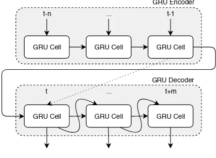
Multi-input and multi-output (MIMO) inferencing can be implemented by making use of a sequence to sequence (seq2seq) structure. In seq2seq, the model exists out of two parts, the encoder and the decoder. The encoder is an RNN which encodes an input sequence into a fixed-length vector, which is called a context vector. This vector is the cell state computed after iterating over the whole input sequence, fromt−n untilt−1, wheren is the length of the input. After the input is encoded into a context vec-tor, the decoder receives it as an initial state, each output step can then be computed [30]. During inferencing, the output of the prediction at the previous timestep is fed into the next GRU cell as input, when predicting the first step however, the real-valued output oft−1 is fed intot. During training, instead of feeding the computed output at timestept+xintot+x+ 1, the real-valued output can be given, this is called guided training. Seq2seq is known for its success in natural language processing, but can also be applied to time series (TS) [7]. A diagram of seq2seq can be seen in Figure 2.
GRU Cell GRU Cell GRU Cell
GRU Encoder
GRU Cell GRU Cell GRU Cell
GRU Decoder
t-n ... t-1
t ... t+m
Figure 2. Structure of a sequence to sequence model
2.4
Attention Mechanism
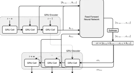
The Attention Mechanism (AM) is an enhancement to the encoder-decoder structure, it was originally proposed by Bahdanau et al. [6] in the context of Neural Machine Translation (NMT). An inherent problem with seq2seq models is that the context vector produced by the en-coder is of a fixed-length, which limits such structures in learning and remembering relevant information in longer sequences, as the amount of information increases as the sequence increases in size, but the size of context vector does not. The performance of seq2seq models suffers sig-nificantly with the length of sequences in the context of NMT [9]. AM was proposed to address this problem. AM works as follows: instead of the context vector be-ing passed only once at the start of decodbe-ing, a unique context vectorcvt is calculated at every time step t. All
the intermediate hidden states from the encoder are used for this [h1, ...ht−1]. A separate ANN receives all
inter-mediate internal states of the encoder and the internal state of the decoder from the previous time step as an input and calculates a score for each of the intermediate state [s1, ...st−1]. Afterwards, the scores are normalized
[image:2.595.65.273.440.509.2]a single decoding step is calculated by multiplying each attention weight with its corresponding state and sum-ming all the resulting vectors together. A diagram of an encoder-decoder structure with attention can be seen in Figure 3.
GRU Cell GRU Cell GRU Cell GRU Encoder
GRU Cell GRU Cell GRU Cell GRU Decoder
− ... − 1
+ ...
Feed Forward Neural Network
ℎ−1
[ℎ−, . . . ,ℎ−1]
[−, . . . , −1]
Softmax [−, . . . , −1]
= [−∗ℎ−, . . . , −1∗ℎ−1]
+
ℎ+
Figure 3. Structure of seq2seq model with Atten-tion
3.
RELATED WORK
In this section we will cover prior research and other work related to the topic of building energy prediction and ma-chine learning. In the end we will mention the possible impact this research can have in the area of creating more accurate building energy prediction models.
3.1
Neural Networks
In 1991, Kreider [23] did research into the viability of ANNs for buildingn energy prediction when the ANN was still relatively new. They found that the ANN could pre-dict future energy usage with good accuracy.
A paper by Yang et al. [32] analyzes the accuracy that a vanilla ANN has for short-term load forecasting compared to RNNs. The papers also compares the ANN and RNNs to several most commonly used methods for energy pre-diction. These are support vector regression (SVR) [8], decision trees (DT) [18], autoregressive integrated moving average model (ARIMA) [5] and random forest (RF) [20]. This research concluded that the NNs outperformed all the baseline models, with the RNN being the most effective in short-term load forecasting.
3.2
RNN Variations and Inferencing
Quite some research has already been done into the appli-cation of RNNs for building energy prediction. In a paper by Fan et al. [15], many different strategies of implement-ing RNNs for TS in the context of energy prediction were investigated. This research compares the ”vanilla” RNN, GRU and LSTM with each other for three different in-ferencing methods. These inin-ferencing methods being the recursive approach, the direct approach and the MIMO ap-proach, the latter approach being achieved with seq2seq. The study concludes that the GRU and LSTM outperform the ”vanilla” RNN, but have comparable performance to one another. The GRU however did have faster compu-tation times. This research also concluded that the direct approach outperforms the recursive and MIMO approach. However, the MIMO approach showed promising results.
3.3
Convolutional Neural Networks
CNNs are used in combination with RNNs in a paper by Fan et al. [15]. They concluded that the CNNs did not necessarily impact accuracy but can significantly re-duce the overall training time. A paper by Maggiolo and
Spanakis [26] however, investigates the use of a multi-scale CNN (MS-CNN). They show that the combination of a CNN and RNN can be very effective. They concluded that a feature extractor was more effective than a simple recurrent encoding in the case of MTS.
3.4
Contribution
This research focuses on creating building energy predic-tion models with RNNs using MIMO inferencing, which is a state-of-the-art inferencing approach that was intro-duced in 2014 by Sutskever et al. [30], which will be achieved with seq2seq. To improve these models even further, an-other state-of-the-art technique is implemented, AM, which was introduced by Bahdanau et al. [6] as an enhancement to existing seq2seq structures. Lastly, 1d-convolutions are used to investigate its potential impact on accuracy, but most importantly, its impact on computation time. All of these techniques are then analyzed on four different ag-gregation levels, in order to determine what impact these techniques can have on the accuracy, when there is a dif-ferent frequency of sudden fluctuations within the data.
4.
RESEARCH QUESTIONS
In this research the following research questions will be answered. RQ1 will be answered first, but before RQ1 is answered, the three subpoints will be investigated. After RQ1, RQ2 can be answered.
RQ1To what extent can we build energy prediction mod-els using RNNs?
RQ1.1Can we implement a seq2seq for making energy predictions?
RQ1.2Can we implement convolutional operations for our seq2seq model?
RQ1.3Can we implement AM for our seq2seq model?
RQ2 How do these machine learning techniques impact the performance of the models?
5.
METHODOLOGY
5.1
Data
The data used for this research is from the Pecan Street Inc. database [3]. There are two categories of data col-lected. The first category contains the building energy consumption data, which is collected on 15-minute inter-vals. For this category, data from 121 buildings was col-lected, in total spanning two years, from 2014-2015. All buildings are located in Austin, Texas, and mostly consist of residential buildings, containing single-family homes. An excerpt of the aggregated data from the 121 buildings can be seen in Figure 4.
The average energy usage on a day of all buildings can be seen in Figure 5.
Figure 4. Example of total building energy use for one day for 121 buildings.
Figure 5. Average energy pattern throughout a day of 121 buildings
hour, the missing datapoints for the 15-minute intervals are interpolated. In total, ten meteorological variables are considered, these are summarized in the Table 1.
Additionally, three more features, which describe the time of the observations, are added, i.g. month, weekday and hour. In order to represent the cyclic nature of time, each of these features is converted into two variables, these two variables represent the sine and cosine of the time feature, calculated as in Equation 1 and 2.
sin(t) =sin(2π·t/T) (1)
cos(t) =cos(2π·t/T) (2) WhereT is the total amount of time units.
In order to prepare the data, NumPy[1] and Pandas[2] are used. The data is split in half to create the testing and training sets. The entirety of 2014 is used for the training set and the entirety of 2015 is used for the testing set. From the collected data, four different datasets are created with different building aggregation levels, i.g. 1, 25, 50 and 75. Each dataset is then merged with the meteorological data, where the meteorological data is interpolated to fill the 15 minute resolution.
[image:4.595.59.281.272.437.2]Meteorological variables Range Mean Temperature [20.7-102.9] 68.1 Dew point [2.8-77.3] 56.3 Humidity [0.11-0.99] 0.70 Visibility [0.3-10.0] 9.3 Apparent temperature [9.1-107.7] 68.4 Pressure [996.7-1042.8] 1016.6 Wind speed [0.00-23.55] 5.64 Cloud cover [0.00-1.00] 0.36 Precipitation intensity [0.000-0.568] 0.004 Precipitation probability [0.00-1.00] 0.06
Table 1. Summary of meteorological variables
After these preparatory steps the data is normalized. The mean (µ) and standard deviation (σ) of each feature is calculated and the data is normalized by means of feature standardization. Feature standardization is described as in Equation 3.
x0= x−µ
σ (3)
Where x is the original value, and x0 is the computed standardized value.
5.2
Proposed network structures
Each proposed network has an input layer that receives 96 timesteps, amounting to an input sequence with a length of 24 hours, and 83 features, representing the energy, weather and time features as described in the previous section. The networks output 96 timesteps as well, making predictions on a 24-hour prediction horizon.
Five different structures are evaluated. As a baseline, a simple ANN is used. The ANN has three dense layers, the amount of hidden units per layer being 1024, 256 and 96 respectively.
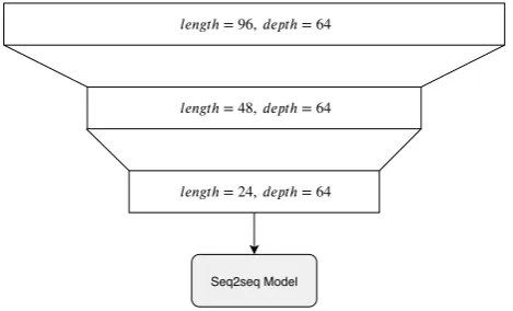
There are four flavours of seq2seq models that were evalu-ated in this research. The first is a seq2seq model without any additions. The state size is 128 (as is with all the other seq2seq models). Next a seq2seq model is built with 1-dimensional convolutions as an addition. Two convo-lutional layers are used, both reducing the length of the given sequence to half of its original size. The convolu-tional layers make use of 64 filters. A representation of the convolutional layers can be seen in Figure 6.
ℎ = 96, ℎ = 64
ℎ = 48, ℎ = 64
ℎ = 24, ℎ = 64
Seq2seq Model
Figure 6. Structure of a seq2seq model with con-volutions
[image:4.595.308.543.560.702.2]For the seq2seq models, guided training is used. However, to ensure the models don’t become overly reliant on the previous output, some noise is added to the inputs of the decoder. The noise generated is Gaussian noise, with a standard deviation of 0.2.
5.3
Training
To build and train the models, Keras [11] is used with Tensorflow [4] as the backend. All of the code can be found on github1. Some parameters were selected to train the models with. In order to make a fair comparison, each model is trained with the same parameters. Each model makes use of the Adam optimizer [22] and they are trained with a learning rate of 0.00045. Each model is trained for a maximum of 300 epochs, with 50 steps per epoch and a batch size of 128. An early-stopping mechanism was implemented with a patience of 20, to prevent the network from overfitting. Meaning that if there is no improvement over the validation data for 20 iterations, the training will terminate. The loss function used is mean squared error (MSE).
5.4
Performance evaluation
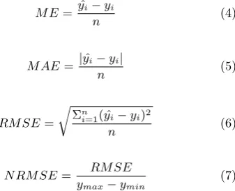
For the performance evaluation we look at two aspects, i.g. the prediction accuracy and computation time. To evaluate the accuracy of the models, we look at two differ-ent aspects. The first aspect is the performance over the whole prediction horizon. The second aspect is the per-formance at each timestep. To measure the perper-formance over the whole prediction horizon we use five different ac-curacy metrics. First of all, we use the normalized root mean squared error (NRMSE), this allows us to express the error of the model in a percentage. Additionally we will also look at the mean error (ME) and the standard deviation (SD), in order to evaluate if a model predicts too high or too low on average and how variable its outcomes are. Lastly, we look at the mean absolute error (MAE) and the root mean squared error (RMSE). All models are compared for all mentioned aggregations.
The second aspect is measured by evaluating the models with their RMSE at each timestep. The equations for the accuracy metrics can be found in Equations 4-7, in which
yis the real-valued output and ˆyis the predicted output.
M E=yˆi−yi
n (4)
M AE= |yˆi−yi|
n (5)
RM SE=
r
Σn
i=1( ˆyi−yi)2
n (6)
N RM SE= RM SE
ymax−ymin
(7)
The performance over the whole prediction horizon and the performance at each timestep is evaluated on the same selection of sequences from the testing data. This data is selected such that each possible starting point in a day appears as much as any other starting point.
Lastly, in order to evaluate the computation time, we take the mean and standard deviation of the time it takes to complete an epoch in seconds and compare these results.
1https://github.com/MaukWM/energy_prediction
[image:5.595.311.537.484.649.2]6.
RESULTS
Table 2 shows the accuracy of each proposed network with the metrics mentioned in in previous section. For the seq2seq models, the ”-1dconv” addition indicates the model included one dimensional convolutions. The ”-a” addition indicates the model included attention. In the table, mod-els are grouped by aggregation level. For each metric, the model with the best performance in that metric is high-lighted. The accuracies reported in the table are calcu-lated with a 24-hour (96-step) ahead prediction on the testing set. For an aggregation level of 1, the ANN out-performs the seq2seq models. But at higher aggregation levels (i.g. 25, 50 and 75) the ANN is outperformed by the seq2seq models.
In general, attention does not seem to add much to in-crease the performance of the model, being better in some cases but not all. At an aggregation level of 25, the seq2seq model with attention and 1d-convolutions is the best per-forming model. For an aggregation level of 75, attention actually seems to be detrimental to the model, greatly im-pacting its accuracy compared to seq2seq models without attention.
Overall, for the higher aggregation levels (i.g. 50 and 75), the seq2seq models without attention outperform all of the other models in most metrics. For the seq2seq models without attention, 1d-convolutions don’t seem to add any significant impact to the accuracy, this is the case for any aggregation levels.
The ME of each model at almost all aggregation levels is negative, indicating that most models predict a lower energy use than what it is in actuality. This can be a consequence of the models, but can also be a consequence of the testing data (e.g. higher peaks in 2015 because of external factors, like temperature, or increase in use of EVs).
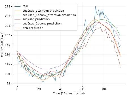
[image:5.595.115.284.526.663.2]An example of a building energy prediction for an aggre-gation level of 25 can be seen in Figure 7. More examples can be found for other aggregation levels in Appendix B
Figure 7. Example of predictions for an aggrega-tion level of 25
As can be seen from the example predictions, the models can predict the trend relatively well, but most fluctua-tions remain unpredicted. For an aggregation level of 1, the models don’t fully predict peaks, as the data is very chaotic. However, in general the models can slightly follow trends of peaks.
Agg Model RMSE NRMSE ME SD MAE
1 ANN 1.10 4.52% -0.02 1.10 0.68
s2s 1.18 4.85% 0.02 1.18 0.72
s2s-1d 1.16 4.78% -0.07 1.16 0.69
s2s-a 1.16 4.80% -0.04 1.16 0.71
s2s-1dconv-a 1.16 4.77% -0.12 1.15 0.68
25 ANN 7.15 6.70% -1.21 7.05 5.33
s2s 6.96 6.52% -0.65 6.93 5.25
s2s-1d 7.17 6.71% -1.05 7.09 5.34
s2s-a 7.28 6.82% -1.59 7.10 5.41
s2s-1dconv-a 6.91 6.47% -0.56 6.89 5.13
50 ANN 11.76 6.06% -3.18 11.33 8.69
s2s 11.20 5.77% -1.75 11.06 8.45
s2s-1d 11.43 5.88% -1.93 11.26 8.41
s2s-a 11.64 6.00% -1.04 11.59 8.68
s2s-1dconv-a 11.76 6.06% -1.21 11.70 8.71
75 ANN 18.77 6.75% -4.58 18.20 13.95
s2s 15.66 5.63% -2.84 15.40 11.51
s2s-1d 15.16 5.45% -3.65 14.72 11.12
s2s-a 23.24 8.36% -5.37 22.61 17.72
[image:6.595.57.541.53.305.2]s2s-1dconv-a 21.51 7.73% -4.68 20.99 16.45
Table 2. Accuracy of predictions for each approach
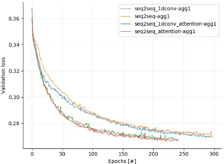
[image:6.595.58.281.476.639.2]attention were on par with the seq2seq models without attention in terms of performance. However, the seq2seq models with attention did converge faster than the seq2seq models without attention, as can be seen in Figure 8. This did not occur for other aggregation levels. In Appendix C other graphs can be found for the validation loss after ev-ery epoch. These graphs exclude the validation loss of the ANN, as the ANN increases the scale by a large factor, making the validation losses for the seq2seq models un-readable. The trends in the graphs stop early because of the implemented early-stopping mechanism.
Figure 8. Validation loss for seq2seq models for an aggregation level of 1
When observing the NRMSE at each aggregation level, the error declines the higher the aggregation level becomes (considering the best models at each aggregation level). Interestingly enough, an aggregation level of 1 seems to get the best performance, when expressed with NRMSE. This can be caused by consistent low levels of energy con-sumption throughout the day, when there is little to no activity. Models are able to predict this trend relatively
well, which results in a very low RMSE, with most of the error coming from short and sudden peaks.
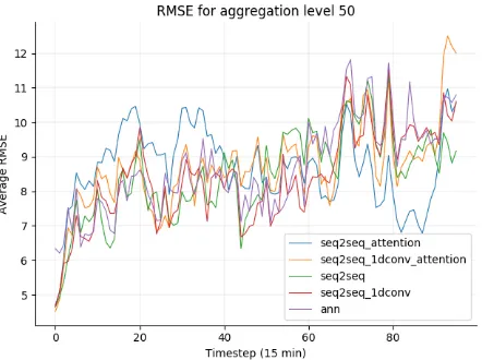
In Appendix A there are four graphs, which show the aver-age RMSE per step for each aggregation level. In general, for each aggregation level, there is a trend of error accu-mulation overtime. These graphs add to the result from Table 2. It is clear from Figure 12 that the seq2seq mod-els without attention, for aggregation level 75, accumulate the error at a lesser rate than the seq2seq models with attention. Interestingly enough, this error accumulation spikes from timesteps 20-40, after which it decreases. In Table 3, the average training time per epoch can be seen for each model in seconds.
[image:6.595.368.487.497.562.2]Model mean(µ) std(σ) ANN 4.20 0.26 s2s 11.84 0.43 s2s-1d 8.08 0.16 s2s-a 76.73 1.57 s2s-1d-a 23.23 0.26
Table 3. Training time per epoch in seconds
The ANN is the fastest model to train, while the seq2seq models require much more time to complete an epoch. This is because in a seq2seq model, each intermediate state must be calculated consecutively, removing the possibility to perform calculations concurrently. The models with attention implemented require a lot more time per epoch. The seq2seq models with 1d-convolutions require less time to train per epoch. Convolutions can be computed in par-allel, thus shortening the sequence that must be computed consecutively. This makes 1d-convolutions an effective ad-dition to reduce time required per epoch, without having a negative impact on the model.
6.1
Discussion
trained longer. For this research a maximum of 20 it-erations was chosen as the cut-off point. In Figure 18 (Appendix C), it can be observed that the validation loss for the seq2seq models with attention, on an aggregation level of 75, starts to increase around epoch 15. At epoch 25 the validation loss stops rising and stabilizes, these mod-els could potentially have improved more but due to the chosen early-stopping policy the models had no chance to improve. Tweaking this number and allowing the models to train longer could result in better models.
To produce the results, only one run was done with each model. This does not always produce reliable results, es-pecially when using an early-stopping policy. The initial-ization of the model can have influence on the speed and the level at which it converges.
Currently, all predictions were done on a 24-hour predic-tion horizon. With seq2seq inferencing however, longer forecasts can be made without having to alter the model in any way. It is possible to make longer predictions with a model trained for 24-hour predictions, this however, is unlikely to produce good results the larger the predic-tion horizon becomes. The model trained to make 24-hour ahead predictions can be used as a starting point to continue training on longer prediction horizons. Without having to change the structure, the model does not have to start all over when training for new predictions horizons.
7.
CONCLUSION
In this paper, four neural network based methods are pro-posed for multi-step day-ahead building energy prediction, and furthermore benchmarked with the well known ANN method. All proposed method are tested using real-world data with a 15 minute resolution. Independent of the building aggregative level, the evaluation shows very good results with all models achieving less than 9% error. On high aggregation levels (i.g. 50 and 75) some of the best performing models achieve less than 6% error. In addi-tion, a deeper look into the convergence capabilities of the models provide us with more insides into the computa-tional requirements of the proposed models.
More specifically, this research investigates the MIMO in-ferencing approach for recurrent models on creating build-ing energy prediction models. Additionally 1d-convolutions and the Attention Mechanism are investigated, to see if these can improve the performance of the models. The models were assessed on four different aggregation levels, i.g. 1, 25, 50 and 75. The MIMO approach seems to be more effective for higher levels of aggregation than a standard ANN, achieving a better performance than the ANN on the three highest aggregation levels. The Atten-tion Mechanism did not seem to improve the accuracy of the seq2seq models at any aggregation level, and was even detrimental to the performance at a high aggregation level of 75. This might indicate that a recurrent model already has enough capacity to learn the temporal dependencies that exist within the building energy prediction problem. However, the Attention Mechanism shows promise at low aggregation levels, as the seq2seq models with attention converged faster than the seq2seq models without atten-tion. Additionally, it is shown that 1d-convolutions are an effective way of reducing the time required to train a seq2seq model per epoch, without having a negative im-pact on the model. This method of reducing training time per epoch is not limited to a model with MIMO infer-encing, but can be applied to any inferencing technique that requires consecutive computations (e.g. the recursive approach or the direct approach).
7.1
Recommendations/Future work
For future work there are many aspects that can still be investigated or improved. Some possible additions that could improve the speed of convergence and reduce over-fitting are regularization, dropout, or batch normalization, of which the latter can now also by applied to RNNs with techniques proposed by Cooijmans et al. [14] or Lei Ba et al. [25].
Other aspects that could be researched are different pre-diction horizons and different resolutions of data. Our results also suggest that the Attention Mechanism may be very useful for building energy prediction with lower resolution (e.g. 1 min, 5 min), where the energy pattern has a larger number of fluctuations (a higher level of non-linearity and uncertainty).
Another way to possibly improve the models is to investi-gate the impact of different recurrent cells for the accuracy of seq2seq models (e.g. ”vanilla” RNN, LSTM).
Another part of the models that can be optimized is the state size. Currently, a state size of 128 is used, but the models could have a better performance with a different state size.
Since MIMO inferencing is used, the seq2seq models can consume and produce sequences of any length. For fu-ture research, it could be valuable to investigate the per-formance of different models on different input and out-put sequence lengths, on which the models have not been trained, to see if this can increase performance without having to train models on lengthy sequences.
For future research it can be valuable to investigate to what extent 1d-convolutions can be used. For example, investigating to what extent the input sequence can be reduced without impacting accuracy. Possibly also inves-tigating the viability of reducing input sequences with 1d-convolutions with other inferencing techniques.
8.
ACKNOWLEDGEMENTS
First, I would like to thank my supervisor, Elena Mocanu, for her valuable feedback, supervision, and also for provid-ing me with readprovid-ings and other materials, greatly helpprovid-ing me to write this research paper. Secondly, I would like to thank Gerben Meijer for his support and advice through-out the course of this research.
9.
REFERENCES
[1] Numpy.http://www.numpy.org/. Software available from numpy.org.
[2] Pandas.https://pandas.pydata.org/. Software available at pandas.pydata.org.
[3] Pecan street inc. dataport.
https://www.pecanstreet.org/. [Online]. [4] M. Abadi et al. TensorFlow: Large-scale machine
learning on heterogeneous systems, 2015. Software available from tensorflow.org.
[5] M. S. Al-Musaylh, R. C. Deo, J. F. Adamowski, and Y. Li. Short-term electricity demand forecasting with mars, svr and arima models using aggregated demand data in queensland, australia.Advanced Engineering Informatics, 35:1–16, 2018.
[6] D. Bahdanau, K. Cho, and Y. Bengio. Neural machine translation by jointly learning to align and translate.arXiv preprint arXiv:1409.0473, 2014. [7] G. Bontempi. Long term time series prediction with
[8] E. Ceperic, V. Ceperic, and A. Baric. A strategy for short-term load forecasting by support vector regression machines.IEEE Transactions on Power Systems, 28(4):4356–4364, 2013.
[9] K. Cho, B. Van Merri¨enboer, D. Bahdanau, and Y. Bengio. On the properties of neural machine translation: Encoder-decoder approaches.arXiv preprint arXiv:1409.1259, 2014.
[10] K. Cho, B. Van Merri¨enboer, C. Gulcehre, D. Bahdanau, F. Bougares, H. Schwenk, and Y. Bengio. Learning phrase representations using rnn encoder-decoder for statistical machine translation.arXiv preprint arXiv:1406.1078, 2014. [11] F. Chollet et al. Keras.https://keras.io, 2015. [12] J. Chung, C. Gulcehre, K. Cho, and Y. Bengio.
Empirical evaluation of gated recurrent neural networks on sequence modeling.arXiv preprint arXiv:1412.3555, 2014.
[13] K. Clement-Nyns, E. Haesen, and J. Driesen. The impact of charging plug-in hybrid electric vehicles on a residential distribution grid.IEEE Transactions on power systems, 25(1):371–380, 2010.
[14] T. Cooijmans, N. Ballas, C. Laurent, ¸C. G¨ul¸cehre, and A. Courville. Recurrent batch normalization.
arXiv preprint arXiv:1603.09025, 2016.
[15] C. Fan, J. Wang, W. Gang, and S. Li. Assessment of deep recurrent neural network-based strategies for short-term building energy predictions.Applied Energy, 236:700–710, 2019.
[16] I. Goodfellow, Y. Bengio, and A. Courville.Deep learning. MIT press, 2016.
[17] R. H. Hahnloser, R. Sarpeshkar, M. A. Mahowald, R. J. Douglas, and H. S. Seung. Digital selection and analogue amplification coexist in a cortex-inspired silicon circuit.Nature, 405(6789):947, 2000. [18] A. Hambali, M. Akinyemi, and N. JYusuf. Electric
power load forecast using decision tree algorithms.
Comput. Inf. Syst. Dev. Informatics Allied Res. J., 7(4):29–42, 2016.
[19] S. Hochreiter and J. Schmidhuber. Long short-term memory.Neural computation, 9(8):1735–1780, 1997. [20] J. Huo, T. Shi, and J. Chang. Comparison of
random forest and svm for electrical short-term load forecast with different data sources. In2016 7th IEEE International Conference on Software Engineering and Service Science (ICSESS), pages 1077–1080. IEEE, 2016.
[21] R. Irle. Global ev sales for 2018 - final results.
http://www.ev-volumes.com/news/
global-ev-sales-for-2018/, 2019. [Online; accessed May 2, 2019].
[22] D. P. Kingma and J. Ba. Adam: A method for stochastic optimization.arXiv preprint arXiv:1412.6980, 2014.
[23] J. Kreider. Artificial neural networks demonstration for automated generation of energy use predictors for commercial buildings.Ashirae Transactions, 97(1):775–779, 1991.
[24] Y. LeCun, L. Bottou, Y. Bengio, P. Haffner, et al. Gradient-based learning applied to document recognition.Proceedings of the IEEE, 86(11):2278–2324, 1998.
[25] J. Lei Ba, J. R. Kiros, and G. E. Hinton. Layer normalization.arXiv preprint arXiv:1607.06450, 2016.
[26] M. Maggiolo and G. Spanakis. Autoregressive
convolutional recurrent neural network for univariate and multivariate time series prediction.
arXiv preprint arXiv:1903.02540, 2019.
[27] D. Palaz, R. Collobert, et al. Analysis of cnn-based speech recognition system using raw speech as input. Technical report, Idiap, 2015.
[28] L. P´erez-Lombard, J. Ortiz, and C. Pout. A review on buildings energy consumption information.
Energy and buildings, 40(3):394–398, 2008. [29] D. E. Rumelhart, G. E. Hinton, R. J. Williams,
et al. Learning representations by back-propagating errors.Cognitive modeling, 5(3):1, 1988.
[30] I. Sutskever, O. Vinyals, and Q. V. Le. Sequence to sequence learning with neural networks. InAdvances in neural information processing systems, pages 3104–3112, 2014.
[31] J. Yang, M. N. Nguyen, P. P. San, X. L. Li, and S. Krishnaswamy. Deep convolutional neural networks on multichannel time series for human activity recognition. InTwenty-Fourth International Joint Conference on Artificial Intelligence, 2015. [32] L. Yang and H. Yang. Analysis of different neural
Appendices
[image:9.595.314.535.55.222.2]A.
AVERAGE RMSE PER TIMESTEP
[image:9.595.60.280.107.273.2]Figure 9. Average RMSE per timestep for an ag-gregation level of 1
Figure 10. Average RMSE per timestep for an
aggregation level of 25
Figure 11. Average RMSE per timestep for an
[image:9.595.314.536.321.484.2]aggregation level of 50
Figure 12. Average RMSE per timestep for an
aggregation level of 75
B.
EXAMPLE PREDICTIONS
Figure 13. Example of predictions for an aggrega-tion level of 1
[image:9.595.60.280.339.503.2] [image:9.595.313.537.567.735.2] [image:9.595.60.281.568.733.2]Figure 15. Example of predictions for an aggrega-tion level of 75
C.
VALIDATION LOSSES
[image:10.595.312.536.57.222.2]Figure 16. Validation loss for seq2seq models for an aggregation level of 25
[image:10.595.59.280.317.483.2]Figure 17. Validation loss for seq2seq models for an aggregation level of 50
[image:10.595.57.282.568.733.2]