warwick.ac.uk/lib-publications
Original citation:Pollicott, Mark and Vytnova, P.. (2015) Estimating singularity dimension. Mathematical Proceedings of the Cambridge Philosophical Society, 158 (2). pp. 223-238
Permanent WRAP URL:
http://wrap.warwick.ac.uk/79584
Copyright and reuse:
The Warwick Research Archive Portal (WRAP) makes this work by researchers of the University of Warwick available open access under the following conditions. Copyright © and all moral rights to the version of the paper presented here belong to the individual author(s) and/or other copyright owners. To the extent reasonable and practicable the material made available in WRAP has been checked for eligibility before being made available.
Copies of full items can be used for personal research or study, educational, or not-for profit purposes without prior permission or charge. Provided that the authors, title and full bibliographic details are credited, a hyperlink and/or URL is given for the original metadata page and the content is not changed in any way.
Publisher’s statement:
© 2015 Cambridge University Press.
http://dx.doi.org/10.1017/S030500411400053X
A note on versions:
The version presented here may differ from the published version or, version of record, if you wish to cite this item you are advised to consult the publisher’s version. Please see the ‘permanent WRAP url’ above for details on accessing the published version and note that access may require a subscription
Estimating Singularity Dimension
M. Pollicott and P. Vytnova
University of Warwick
∗Abstract
In this article we address an interesting question on the computation of the dimen-sion of self-affine sets in Euclidean space. A well known result of Falconer showed that under mild assumptions the Hausdorff dimension of typical self-affine sets is equal to its Singularity dimension. Heuter and Lalley subsequently presented a smaller open family of non-trivial examples for which there is an equality of these two dimensions. In this article we analyse the size of this family and present an efficient algorithm for estimating the dimension.
1
Introduction
Despite the prominent role played by Hausdorff dimension in both analysis and dy-namical systems, there remain very few non-trivial examples for which the value of dimension can be explicitly stated, or even effectively computed. There has been some success in the case of conformal iterated function schemes [7] and [4], but considerably less in the case of non-conformal maps.
On the other hand there is a very elegant result of Falconer which shows that the Hausdorff dimension of the limit set for a typical finite set of (non-conformal) affine contractions is equal to the singularity dimension, whose presentation is more suggestive of allowing estimation of the value. However, even this doesn’t necessarily lend itself to numerical evaluation. In this note we want to consider a particular setting, introduced by Hueter and Lalley, where they showed that the singularity dimension is always equal to the Hausdorff dimension. In this case we shall describe a very effective method for its rapid numerical evaluation.
We begin by recalling the general setting in which we will be working.
Notation 1.1. Let A1,· · ·, Ak ∈ GL(2,R) be 2×2 invertible matrices and assume
that kA1k,· · ·,kAkk< 12. Given vectors b1,· · ·, bk ∈ R2 we can consider affine maps
Ti :R2 →R2 defined by Ti(x) =Aix+bi (i= 1,· · ·, k).
We next give a basic definition.
Definition 1.2. The limit set Λ ⊂ R2 is the unique smallest closed non-empty set
such that Λ =T1Λ∪ · · · ∪TkΛ.
1 INTRODUCTION
Falconer introduced the notion of the singularity dimension dimS(Λ), which is
typ-ically equal to the Hausdorff dimension, but while having a better implicit characteri-zation is still remarkably difficult to estimate numerically.
Notation 1.3. If n≥1 and i= (i1,· · ·, in)∈ {1,· · ·, k}n, then we write |i|=n. We
can then associate to i the product of matrices Ai =Ai1Ai2· · ·Ain.
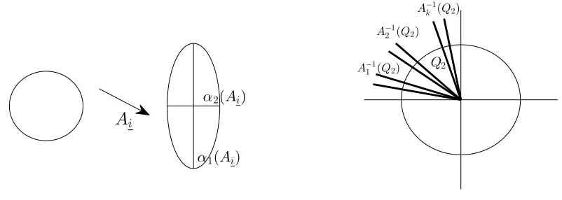
We can associate to the 2×2 matrixAi the two singular values α1(Ai)≥α2(Ai).
These are the major and minor axes of the ellipse which is the image of the unit circle underAi. Equivalently, these are the eigenvalues of the 2×2-matrix
q
A∗iAi [1].
Definition 1.4. We denote
φs(Ai) =
(
α1(Ai)s if 0< s≤1
α1(Ai)α2(Ai)1−s if 1≤s <2.
This leads to the following definition of singularity dimension due to Falconer.
Definition 1.5. We define the singularity dimension by
dimS(Λ) : = inf
s >0 :
∞
X
n=1
X
|i|=n
φs(Ai)<+∞
.
We now recall the following fundamental theorem of Falconer.
Theorem 1.6(Falconer [1]). Assume thatkA1k,· · · ,kAkk< 12. Then for a.e. (b1,· · · , bk)∈
R2k, we have dimH(Λ) = dimS(Λ).
In fact, Falconer proved the result under some slightly more restrictive assumptions, which were removed by Solomyak [11]. The significance of this result is that the formula holds quite generally: for any contractions with Euclidean norm less than 12; and almost all translational parts. On the other hand, except in very special cases it is not always easy to give explicit examples to which the formula applies. Heuter and Lalley showed that under more restrictive hypotheses on the maps it is possible to remove the almost everywhere hypothesis.
Let Q2={(x, y) : x≤0, y ≥0} denote the closed second quadrant
Hypotheses 1.7 (Heuter–Lalley conditions). We want to assume the following tech-nical conditions:
1. kAik<1 for i= 1,· · · , k;
2. α1(Ai)2 < α2(Ai) for i= 1,· · ·, k;
3. A−11Q2,· · · , Ak−1Q2 are pairwise disjoint subsets of int(Q2);
4. there is a bounded open set V such that TiV are disjoint, i= 1,· · · , k.
Conditions (1)–(3) depend only on the Ai, but condition (4) also depends on the
bi. (An additional simplifying assumption would be thatA1,· · ·, Ak have positive
de-terminants.) Condition (1) is a weaker contraction hypothesis than in Theorem 1.6. Condition (2) is a bunching condition; condition (3) a separation condition. Condi-tion (4) is a closed set condiCondi-tion. Next, we recall the result of Heuter–Lalley.
Theorem 1.8 (Heuter–Lalley [3]). Under Hypotheses 1.7 we have that
1 INTRODUCTION
α1(Ai) α2(Ai)
A
iA−1
1 (Q2)
A−1
2 (Q2)
A−1 k (Q2)
[image:4.612.104.505.90.233.2]Q2
Figure 1: The singularities of the matrix Ai and a few images of the second quadrant.
However, it remains to address the question of effectively estimating the dimension. Our main result is the following
Theorem 1.9 (Main Theorem). Under Hypotheses 1.7 there exists 0 < θ < 1 such that we can define a sequencedn using the2n+1 singularities{α1(Ai) : |i| ≤n}so that
|dimS(Λ)−dn|=O
θn2
for n≥1.
In particular, we see that the rate of convergence of then’th approximation to the dimension is super exponential, whereas the number of terms needed to compute is exponential.
Example 1.10. Heuter and Lalley proposed the matrices
A1 =
1
30 1 120 1 30
1 60
, A2 =
1
30 1 40 1 30
1 30
, A3 =
1
40 1 30 1 60
1 30
.
It is easy to show that for suitable translations Heuter–Lalley conditions hold. More-over, we estimate that the dimension of the limit set is
dimS(Λ) = 0.375797704495199. . .
using products of the length 5, so we need to calculate only 35 = 243 matrices overall.
It can be difficult to find explicit examples of matrices satisfying the Heuter–Lalley conditions (Hypotheses 1.7 ). It is an interesting question to ask how likely it is that a family randomly chosen matricesA1, . . . , Ak satisfy them. We will discuss this in the
next section.
In §2 we consider how restrictive hypothesis 1.7 are. In particular, we consider the probability that ak-tuple of matrices chosen at random with respect to a natural measure has these properties. In §3 we relate to the matrices projective maps, which allows us to use dynamical techniques. In §4 we use this formulation to describe the singularity dimension in terms of thermodynamic formalism. In §5 we describe the main mechanism in the proof, the determinant of the transfer operator and in §6 we complete the proof of the main theorem 1.9. Finally, in §7 we present examples illustrating the rapid convergence in the main theorem.
2 THE LIKELIHOOD OF THE HYPOTHESES
2
The likelihood of the hypotheses
In this section we address the following question: What is the probability thatkmatrices chosen randomly satisfy conditions (1)–(3) of Hypotheses 1.7? In fact, we will see, both empirically and rigorously, that these conditions can be difficult to satisfy, particularly when the number of matrices k is large. On the one hand, if the singular values of two or more of the matrices are sufficiently large then the image of the positive quadrant will be a large sector and part 3 of Hypotheses 1.7 may be impossible to satisfy. We will quantify this in this section. On the other hand, if the singular values of the matrices are all small, it is relatively easy to estimate the probability that a
k-tuple of such matrices satisfy Hypotheses 1.7. In particular, in this case the images of the positive quadrant are very narrow sectors and we could consider the product of their independent distributions. It remains to understand the general case, which we can approach by estimating the number of k-tuples where the singular values have a common lower bound τ, say. We will present formulae for the density of the k-tuples which satisfy the hypotheses, and consider their asymptotic behaviour as the lower bound on the singular values tends to zero. In particular, we will show that there is a simple asymptotic formula (Proposition 2.7) which fits with the empirical results for
k= 1,2.
We begin by presenting a natural parametrization of matrices which is useful for both interpreting Hypotheses 1.7 (1)–(3) and quantifying the probability they are sat-isfied.
Using the Singular Value Decomposition for matrices we can write the inverse of each matrix as
A−i 1 =Rθ1(Ai)
1/α1(Ai) 0
0 1/α2(Ai)
Rθ2(Ai)
whereRθ is rotation by an angleθ. Providedθ2(Ai)∈(0,π2)∪(π,32π) = :I2,ithe image
of Rθ2(Q2) contains the real axis. More precisely, the image cone Rθ2(Q2) is bounded
by lines containing the vectors
−sinθ2(Ai)
cosθ2(Ai)
and
−cosθ2(Ai)
−sinθ2(Ai)
.
The action of the diagonal matrix then squeezes the coneRθ2(Ai)(Q2) inside itself. The
new cone is bounded by lines containing the vectors
−sinθ2(Ai)/α1(Ai)
cosθ2(Ai)/α2(Ai)
and
−cosθ2(Ai)/α1(Ai)
sinθ2(Ai)/α2(Ai)
.
In particular, these lines make angles with the horizontal axes equal to
φ1 := tan−1
α2(Ai)
α1(Ai)
tanθ2(Ai)
and φ2 := tan−1
α2(Ai)
α1(Ai)
cotθ2(Ai)
,
respectively, and the angle for the image cone is given by φ=φ1+φ2. Therefore we
may write
tanφ= α2(Ai)
α1(Ai)
·tanθ2(Ai) + cotθ2(Ai)
1−α2(Ai)
α1(Ai)
2 . (1)
Finally, the map Rθ1(Ai) maps this cone back into the second quadrant Q2 under the
condition thatθ1∈[π2, π]∪[32π,2π] = : I1,i.
2 THE LIKELIHOOD OF THE HYPOTHESES
Lemma 2.1. Given kmatrices such that preimages of Q2 are disjoint, at least one of
them satisfies
α2(Ai)
α1(Ai)
≤
p
1 + tan2(π/2k)−1
tan(π/2k) .
Proof. This is an explicit computation. By (1) the image of Q2 under any A−i 1 is a
cone with angleφthat satisfies
tanφ≥ α2(Ai)
α1(Ai)
· 2
1−α2(Ai)
α1(Ai)
2.
In particular, if there arekdisjoint cones then we require that for at least one choice 1≤
i≤k we have that
tanπ 2k
≥tanφ≥ α2(Ai)
α1(Ai)
· 2
1−α2(Ai)
α1(Ai)
2,
which implies the result.
Example 2.2. For example, in order to have k= 2 matrices with disjoint preimages, we need one of them to satisfy α2(Ai)
α1(Ai) ≤
√
2−1.
We now turn our attention to the likelihood that the hypotheses hold. We assume that parameters defining matricesA−i 1 are uniformly distributed on the corresponding intervals:
Xi: =
n
(α1, α2, θ1, θ2)⊂(0,1)2×I1,i×I2,i
o
. (2)
The probability space is defined by X: =
k
Q
i=1
Xi, where we assume a uniform
distri-bution.
We observe that if α1 1, the contraction is strong and the image of Q2 under A−i 1 is a very narrow cone. Thus, at least quantatively, the probability that k ma-trices satisfy Hypotheses 1.7 is high. We are therefore interested in the probability thatk matrices chosen at random satisfy Hypotheses 1.7 when the singular values are assumed not to be too small. In particular, we want to add an additional condition on singularities 0 < τ ≤α2 ≤α1 < 1 and study the probability that Hypotheses 1.7
(1)–(3) hold true as a function of τ.
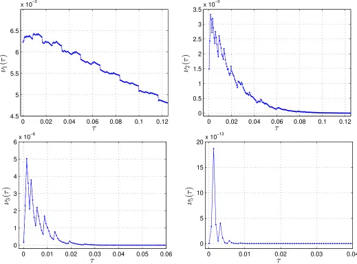
Definition 2.3. We denote by νk(τ) the emprically observed proportion of k-tuples
of matrices satisfying the hypotheses, whereas we denote by Pk(τ) the theoretically
predicted value.
The graphs in Fig. 1 below show the proportionνk(τ) of families ofkmatrices that
satisfy Hypotheses 1.7 among all possible families of k matrices. They are obtained by a routine straightforward computer calculation. More precisely, we take 200 values of τ between 0 and 0.125, and for every τ we consider 50 values of angles θ1 ∈ I1,i,
θ2 ∈ I2,i and 30 values of singularities α1, α2 on the interval (τ,1). Afterwards, we
consider all possible matrices and calculate ν1(τ), the proportion of matrices that
satisfy Hypotheses 1.7 (1)–(3). Then we look for pairs, triples, quartets and quintets. We would like to explain the shape of these empirically observed plots by rigorously estimating the asymptotic behaviour of νk(τ) as τ → 0 and to find the probability
2 THE LIKELIHOOD OF THE HYPOTHESES
0 0.02 0.04 0.06 0.08 0.1 0.12 4.5
5 5.5 6 6.5
x 10−3
τ
ν
1(
τ
)
0 0.02 0.04 0.06 0.08 0.1 0.12 0
0.5 1 1.5 2 2.5 3 3.5
x 10−3
τ
ν
2(
τ
)
0 0.01 0.02 0.03 0.04 0.05 0.06
0 1 2 3 4 5 6
x 10−6
τ
ν
3(
τ
)
0 0.01 0.02 0.03 0.04
0 5 10 15 20
x 10−13
τ
ν
5(
τ
[image:7.612.41.560.76.460.2])
Figure 2: There are plots of the proportion of (a) Heuter–Lalley matrices A; (b) Heuter–
Lalley pairs of matrices (A1, A2); (c) Heuter–Lalley triplets of matrices (A1, A2, A3); and (d)
Heuter–Lalley quintets of matrices (A1,. . . , A5) with singularitiesα1> α2> τ.
Hypotheses (1.7). We start with P1(τ). Let φ(θ1, θ2, α1, α2) be the angle of the cone A−1(Q2). Then
P1(τ) =
Z π
2
0
π
2 −φ
ρφ(x)dx (3)
where ρφ(x) is the probability density function for φ. The following lemma gives us
the density of the distribution for tan(φ).
Lemma 2.4. The random variable tanφ is distributed with density
ρtanφ(x, τ) =
Z x/2
2√τ 1−τ
1
√
2π
y
xpx2−4y2
τ2
u2(y)+ u2(y)
4
u0(y)dy, (4)
where u(x) = √
2 THE LIKELIHOOD OF THE HYPOTHESES
Proof. We can write tanφas a product of independent variables using (1)
tanφ= 2 sin(2θ2)
· α1α2
α2 1−α22
.
To simplify the calculations, we introduce ˜α: = α1α2
α2 1−α22
and ˜θ: = sin(22θ
2). We can
now use standard formulae for the density of the product distribution to approach the density of tanφ. We obtain the density ρθ˜(x) by straightforward calculation.
ρθ˜(x) =
( 1
2π
1
x√x2−4, ifx >2;
0, otherwise.
To calculate the density of ˜α we introduce new a functionu(x) = √
1+4x2−1
2x . Then the
probability P( ˜α < x) is given by the area in the (α1, α2)-plane bounded by the lines α2 =τ,α2=u(x)α1, and parabolaα2=α21. Hence by definition
ρ e
α(x) = lim →0
1
(P(αe≤x)−P(αe≤x+)) = (
τ2
u2(x)+
u2(x) 4
u0(x) ifx >
√
τ
1−τ,
0 otherwise .
Convolvingρθ˜and ρα˜ together, we conclude
ρtan(φ)(x, τ) =
Z
R
1
y·ρθ˜
x
y
ρα˜(y)dy=
Z x/2
√
τ 1−τ
1
√
2π
y
xpx2−4y2
τ2
u2(y)+ u2(y)
4
u0(y)dy,
providedx > 2
√
τ
1−τ.
As a corollary to Lemma 2.4 we have the following asymptotic expansion for
ρtanφ(x, τ) in powers of τ1/2.
Corollary 2.5. There is a power series expansion
ρtanφ(x, τ) =
∞ P j=0
aj(x)τj/2 if x > 2
√
τ
1−τ,
0 otherwise;
which converges uniformly for any x > 2
√
τ
1−τ, and all aj(x) are analytic on the same
domain.
Proof. It suffices to observe that the integrand, and thus its anti-derivative, is analytic at 0 as a function ofx.
Combining 2.1 with 2.4 we get an upper bound for τk: = inf{τ :Pk(x, τ) = 0}:
Corollary 2.6.
τk≤
2 + tan2(π/2k)−2p1 + tan2(π/2k)
tan2(π/2k)
Heuristically, as kincreases we see that at least one of the matrices in the k-tuple must correspond to a small value of α. In particular, this imposes conditions which suggest this is a relatively rare event.
We now use corollary 2.5 to show thatP(τ) has an asymptotic formula in terms of
3 PROJECTIVE MAPS
Lemma 2.7. The probability P(τ) that A(Q2) ⊂ Q2, kAk ≤ 1, and α1(A)2 < α2(A)
subject to α1(A), α2(A) ≥τ > 0 can be expanded as a power series in
√
τ (where the coefficients for√τ and τ vanish).
Proof. The probability that the imageA(Q2) lies back in the quadrantQ2 is
Z π
2
0
π
2 −x
ρφ(x, τ)dx=
Z ∞
0
π
2 −tan
−1(x)ρ
tanφ(x, τ)dx
=
Z ∞
2√τ 1−τ
π
2 −tan
−1(x)ρ
tanφ(x, τ)dx.
We observe that for small τ > 0 the integrand is analytic at x = 2, with radius of convergence 2. In particular, it is analytic at the value of the lower value in the range of integration. Therefore we can expand it in a power series inxatx= 2, and integrate term by term. This gives the result.
Similarly, the probability P2(τ) that the images of two sectors are in the quadrant
is given by
P2(τ) =
2
π
Z π/2
0
Z y
0
(y−x1)ρφ(x1, τ)dx1
Z π2−y
0
π
2 −y−x2
ρφ(x2, τ)dx2
!
dy
can be expanded as a power series in √τ. (We make sure that two sectors are disjoint by putting one of them between the real axis and a ray (0, y) and another one between (0, y) and the imaginary axis). This brings us to an asymptotic expansion for Pk(τ).
Continuing inductively one can show that the probability Pk(τ) that k images of
the quadrant are disjoint takes the following form:
Proposition 2.8. The probabilityPk(τ) to havek matrices satisfying Hypotheses 1.7
(1)–(3) and with singularities at least τ, may be expanded as a power series in√τ.
In view of Proposition 2.8 we can attempt to fit polynomials in √τ to the plots in Figure 2. In Figure 2 we illustrate this for the representative cases of single matrix and triples of matrices.
In summary, the proportion ofk-tuples of matrices satisfying Hypotheses 1.7 is sen-sitive to the restrictions on the singular values (2.6). We can explicitly computePk(τ)
and compare these with the numerical estimates νk(τ). In the case that we allow a
lower bound on the singular values to tend to zero, we get asymptotic estimatesPk(τ)
(in Proposition 2.8).
3
Projective maps
We can introduce a dynamical viewpoint by looking at the projective action of the matrices on RP1. This technique is classical in the study of the ergodic theory of
random matrix products, but will prove to be particularly useful in the present context. The idea is that the linear action of the matrices on R2 induces a map on the real
projective space RP1. We recall that RP1 corresponds to R2− {(0,0)}/ ∼ where we
use define the equivalence relationv∼w if there existsλ∈R− {0}such thatλv=w. Equivalently, we can identifyRP1 with the unit circle inR2 with the antipodal points
identified. It is well known that one can naturally parameterise RP1 locally by using
3 PROJECTIVE MAPS
0 0.02 0.04 0.06 0.08 0.1 0.12 4.5
5 5.5 6 6.5
x 10−3
τ
P1(τ) ν1(τ)
0 0.01 0.02 0.03 0.04 0.05 0.06
0 1 2 3 4 5 6
x 10−6
τ
[image:10.612.66.549.71.253.2]P3(τ) ν3(τ)
Figure 3: The first and the third plots from Figure 1 with approximating polynomial curves
of degree 6 in √τ superimposed.
Let us write each matrix Ai in the form
Ai =
ai bi
ci di
,
whereai, bi, ci, di∈R, then we can associate the linear maps ˇAi :R2 →R2 given by
ˇ
Ai(x, y) = (aix+biy, cix+diy).
The assumption of positivity of the matrices ensures that the first quadrant Q1 =
{(x, y)∈R2:x, y≥0} is preserved by the linear maps. Consider the one dimensional
simplex ∆ = {(x,1−x) : 0 ≤ x ≤ 1} then the linear maps naturally give rise to projective maps Abi : ∆→∆ given by
b
Ai(x,1−x) =
aix+bi(1−x)
aix+bi(1−x) +cix+di(1−x)
, cix+di(1−x)
aix+bi(1−x) +cix+di(1−x)
.
In particular, the first component is a linear fractional mapAi: [0,1]→[0,1] given by
Ai(x) =
(ai−bi)x+bi
(ai+ci−bi−di)x+ (bi+di)
.
Each of these maps is merely the same action on (part of) RP1 viewed using different
coordinates. The strict positivity of the matrices ensures that the images Ai([0,1]) lie
inside the open interval (0,1). Although the fact will not be necessary in our analysis, this is sufficient to ensure that these maps are contracting with respect to a suitable metric. Given the product of 2×2 matrices Ai we can denote its eigenvalues by
λ1(Ai) ≥ λ2(Ai) and then we can write its determinant as their product det(Ai) =
λ1(Ai)λ2(Ai). The rest of this section is devoted to relating the fixed point of the
projective mapAi to the eigenvalues of the matrix Ai.
4 SINGULARITY DIMENSION AND TRANSFER OPERATORS
Lemma 3.1. If vi = (xi,1−xi) is an eigenvector for Ai then xi is a fixed point for
Ai. Moreover, we can write the derivative by
DAi(xi) =
det(Ai)
λ1(Ai)2
.
Proof. This could be deduced indirectly from equation (41) of [3]. However, it can also be seen easily directly by a simple geometric argument. Consider a small -ball
B(vi, ) around vi in R2. The ratio of the areas of the original ball B(vi, ) to its
image Ai(B(vi, )) under the linear map Ai :R2 → R2 is detAi. On the other hand,
we see that Ai maps vi to Ai(vi) = λ1(Ai)vi. Thus, since the point vi is fixed by
Ai a consideration of the area of Ai(B(vi, )) shows the contraction in the projective
distance in a neighbourhood of this fixed point must be approximately
det(Ai)
λ1(Ai)2
.
Lettingtend to zero gives the result.
The next lemma shows that the largest singular value and the largest eigenvalue are of a comparable size.
Lemma 3.2. We can estimate:
α1(Ai)λ1(Ai)
i.e., there exists C≥1 such that C1λ1(Ai)≤α1(Ai)≤Cλ1(Ai), for all strings i.
Proof. This is suggested by comparing equations (23) and (29) in [3]. However, it can be seen directly by considering cones±Q1 associated to the first and third quadrant. It
is immediate to see that the action of the positive matrices is such that the direction of the longest axes of the ellipse image of the unit disk must lie in the image comeAi(Q1).
Moreover, this also contains the eigenvector associated to the largest eigenvalue. One then sees easily the result by considering the contracting maps associated to the pro-jective versions.
4
Singularity dimension and transfer operators
The use of positive matrices and the contracting nature of their projective action has been used by several authors in different contexts, including [9], [8]. This has the advantage that it places us in the context of an expanding real analytic map and thus allows us to employ in§5 the powerful theory of nuclear transfer operators associated to this setting.
In the present context, the hypotheses imply that 0<dimS(Λ)<1. Thus we have
by definition that φs(Ai) =α1(Ai)s and
dimS(Λ) = inf
s >0 : ∞
X
n=1
X
|i|=n
α1(Ai)s<+∞
.
4 SINGULARITY DIMENSION AND TRANSFER OPERATORS
Definition 4.1. Let P :R→R be defined by
P(s) := lim
n→+∞ 1
nlog
X
|i|=n
α1(Ai)s
.
The function P(s) can be viewed as a generalisation of the more familiar pressure function in thermodynamical formalism, which has proved so useful in analysing the Hausdorff dimension of conformal attractors. The mapP :R→Ris a homeomorphism
and its significance is that the singularity dimension dimS(Λ) is then given by the
following result:
Proposition 4.2 ([3], corollary 4.4). The value δ = dimS(Λ) satisfies P(δ) = 0.
By the estimates in the previous section we can see that this is equivalent to the following.
Lemma 4.3. We can write
P(t) := lim
n→+∞ 1
nlog
X
|i|=n
Ψn(i)t
where for convenience we denote Ψn(i) :=
det(Ai)
DAi(xi)
12
.
Proof. By Lemma 3.1 we have that λ1(Ai) =
det(Ai)
DAi(xi)
1/2
and by Lemma 3.2 (1) we have thatα1(Ai)λ1(Ai). The result then follows by taking limits.
We want to relate the pressure to a transfer operator on the Banach space of bounded analytic functions. As with the classical theory of Thermodynamical Formal-ism, the value P(s) will be characterised in terms of the maximal positive eigenvalue of a corresponding linear operator. We first introduce a suitable Banach space upon which the operator acts.
Definition 4.4. Let [0,1]⊂U ⊂C be an open neighbourhood of the unit interval. Let
B ⊂ Cω(U) be the Banach space of bounded analytic functions on U, with respect to the supremum norm kwk= supz∈U|w(z)|.
We could equally well work with the Banach space of square integral analytic func-tions on U, but we use this particular space to be consistent with [10].
We can next associate the bounded operator which we will use to characteriseP(t).
Definition 4.5. Given s ∈ C, we can consider the transfer operator Ls : B → B
defined by
Lsw(z) =
k
X
i=1
ψi(z)sw(Aiz)
where ψi(z) =
detAi
DAi(Aiz)
1/2
.
The above operator is well defined provided the open set U is chosen sufficiently small that the closures of its images are contained inU (i.e.,Ai(U)⊂U fori= 1,· · ·, k)
and also sufficiently small that ψ0, ψ1 : U → C and analytic (i.e., the square root is
applied away from the negative real axis).
5 TRACES AND DETERMINANTS
Lemma 4.6. If t∈R then eP(t) is the spectral radius ofLt.
Proof. Observe that from the definitions, we have that for any finite stringi= (i0, i1,· · ·, in−1)
we have that Ψn(i) = n−1
Q
j=0
ψij(Ai0· · ·Ain−1xi). The result then follows from [10].
5
Traces and Determinants
In this section we will recall some classical results on operators. In many other appli-cations of transfer operators, it is sufficient to consider the transfer operator acting on the Banach space of H¨older continuous functions. In that context, the operators are quasi-compact. However, for our purposes it is important that we are considering a small Banach space of analytic functions for which the transfer operators have smaller spectrum.
We begin with a general definition due to Grothendieck [2] and apply these to the particular case of the transfer operator Lt.
Definition 5.1. We say that an operatorT :B→B on a Banach space is nuclear if: 1. There exist vectors vn∈B with kvnk= 1;
2. There exist linear functionals ln∈B∗ with kl∗nk= 1;
3. There exists an absolutely summable sequence λn∈C,
such that we can write T(v) = ∞
P
n=1
λnvnln(v), for all v∈B.
Such nuclear operators are automatically compact operates and thus consequently have only countably many non-zero eigenvalues, whose only possible accumulation value is 0. In particular, nuclear operators are trace class and we can define their traces in terms of the sum of their eigenvalues. For our present purposes we can also assume that (λn)∞n=1 ∈lp for all p >0.
We recall some properties of these operators that can be easily deduced from more general results of Ruelle [10] (and we refer the reader to Appendices A, B and C of [6] for a useful summary). These are contained in the next two propositions [2].
Proposition 5.2 (Grothendieck, Ruelle). For each t > 0 the operators Lt :B → B
are nuclear and we can explicitly write the trace of the n’th power Ln t as:
trace(Lnt) = X |i|=n
(Ψn(i))t
1−DAi(xi)
for each n≥1.
The proof of this explicit form for the trace trace(Ln
t) is quite explicit. It involves
calculating the eigenvalues, and thus traces, of each of the composition operators as-sociated to the individual contractions Ai and then summing.
We next introduce a family of complex functionsD(z, t) of the complex variablez∈
C, parameterized by a real variablet∈R.
Definition 5.3. We can define the determinant
D(z, t) := exp −
∞
X
n=1 zn
ntrace(L
n t)
!
,
6 PROOF OF THEOREM 1.9
Finally, we recall the following useful result on the analytic domain and expansion of D(z, t).
Proposition 5.4 (Grothendieck, Ruelle). The functionD(z, t) is entire inC2.
More-over, there exists 0< θ <1 such that
D(z, t) = 1 + ∞
X
k=1
ak(t)zk
where |ak(t)|=O(θk
2
).
In order to exploit the nuclearity of the transfer operators it is crucial that we work with the Banach space of analytic functions rather than, say, the more familiar setting of H¨older continuous or continuously differentiable functions. In particular, it is a crucial (but trivial) observation that an analytic function in B remains analytic under composition with the linear mapsAi. This is a simple observation based on such
maps being linear fractional maps, which arises automatically from their construction.
Remark 5.5. We recall that the constant 0< θ <1 is related to the minimal contraction of the Ai, fori= 1,· · · , n. In particular, it can be readily estimated.
6
Proof of Theorem 1.9
The proof of Theorem 1.9 depends on the results in the previous section. The use of determinants to compute Hausdorff dimension appeared in [4] in the context of general hyperbolic repellers (e.g. hyperbolic Julia sets and limit sets of suitable Fuchasian groups). The general principle is the same here, although the application is somewhat different. Let us setz= 1 and then denotingη(t) :=D(1, t) and using Proposition 5.4 we can expand
η(t) :=D(1, t) = ∞
X
k=1 ak(t)
where|ak(t)|=O(θk
2
). The significance of this function is the following simple result.
Lemma 6.1. The value δ = dimS(Λ) is the abscissa of convergence of η(s) (i.e., the
least value for whichη(s) converges to an analytic function for Re(s)> δ)
Proof. By definition, the convergence (or divergence) of the function η(t), for t ∈
R, depends on the growth of the terms trace(Lnt), whose explicit form is given in
Proposition 5.4. However, we can then deduce from Definition 4.1 that for t > 0 the series converges (since the terms tend to zero exponentially fast) and for t < 0 the series diverges (since the terms grow exponentially fast). Finally, the lemma follows by Proposition 4.2.
Next, we can write ηN(t) for the truncation of this series of the form:
ηN(t) := N
X
k=1 ak(t)
for N ≥ 1. Let δN > 0 denote the smallest zero, i.e., ηN(δN) = 0. Thus since for
each t we have |ηN(t)−η(t)| = O(θN
2
) and δ is a simple zero for η(t) we deduce thatδ−δN =O(θN
2
7 THE NUMERICAL ALGORITHM
Remark 6.2. The value of 0< θ <1 in the bound |ηN(t)−η(t)|=O(θN
2
) depends on the hyperbolicity of the projective maps associated to the matrices. It is not simply a bound on the derivatives, since it also reflects the complexification of the maps, but it can be assumed close to this value. The implied constant can also be effectively estimated.
7
The Numerical Algorithm
It remains to show empirically that this method gives an efficient way to estimate δ. In this section we present a basic numerical algorithm resulting from theorem 1.9 and illustrate its efficiency using two examples 7.2 and 7.3.
Consider matrices
Ai =
ai bi
ci di
and i= 1, . . . , k
satisfying the hypotheses (1) – (3) of Hypotheses 1.7.
Step 1. For each n≥1 we can consider a stringi= (i0,· · · , in−1)∈ {1,· · ·, k}n. We
associate the product matrix
Ai =Ai0Ai1· · ·Ain−1(xi) =
ai bi
ci di
,
say, and the linear fractional mapsAi : [0,1]→[0,1] given by
Ai(x) =
(ai−bi)x+bi
(ai+ci−bi−di)x+ (bi+di)
.
Step 2. We can then associate to each string i= (i0,· · · , in−1)∈ {1,· · · , k}n:
1. the determinant detAi;
2. the unique fixed pointAi(xi) =xi;
3. the derivative DAi(xi) of the map at the fixed point;
4. the weight
Φn(i, t) =
det(Ai)
DAi(xi)
!t/2
1 1−DAi(xi)
.
Step 3. We can write
DN(z, t) := exp
−
N
X
n=1 zn
n
X
|i|=n
Φn(i, t)
and expanding the exponential as exp(y) = 1 +y+y2/2 +· · ·+yN/N! +O(yN+1) with
y =−
∞
X
n=1 zn
n
X
|i|=n
7 THE NUMERICAL ALGORITHM
we rewrite this as
DN(z, t) = 1 + N
X
k=1
ak(t)zk+O(zN+1).
Step 4. Settingz= 1 we can define
ηN(t) := 1 + N
X
k=1 ak(t).
LetδN >0 be the smallest positive solution to ηN(δN) = 0.
Remark 7.1 (Comparing with the matrix approach). A more standard approach is to associate to eachN a matrix whose entries are approximations to the derivatives raised to the powertN. In particular, for eachN ≥1 we can solve for tN >0 such that
X
|i|=n
DAi(xi)tN = 1,
say. It then follows, as in [7] that tN → dimH(Λ) at an exponential rate, i.e., there
exists 0< θ <1 such that dimH(Λ) =tN +O(θN).
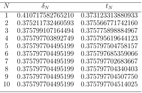
Example 7.2. With the matrices considered in Example 1.10, one can consider the approximations to the dimension using determinants (Theorem 1.9) and compare it with the matrix approximation method (Remark 7.1).
N δN tN
1 0.410717582765210 0.373123313880933
2 0.375211732460593 0.375566771742160
3 0.375799107164494 0.375775898884967
4 0.375797703892749 0.375795619644123
5 0.375797704495199 0.375797504758157
6 0.375797704495199 0.375797685359066
7 0.375797704495199 0.375797702683667
8 0.375797704495199 0.375797704340403
9 0.375797704495199 0.375797704507750
[image:16.612.186.428.394.552.2]10 0.375797704495199 0.375797704514025
Table 1: Approximations for Example 7.2
In particular, we see that for N = 5 the determinant method gives a solution
δ = 0.375797704495199· · ·
which is accurate to15 decimal places. However, even whenN = 10the matrix method is only accurate to9 decimal places.
Example 7.3. With the matrices
A1=
1 26
3 1 2 1
, A2 =
1 26
5 3 5 6
and A3=
1 26
4 5 2 9
7 THE NUMERICAL ALGORITHM
N δN tN
1 0.609325221387553 0.514374159566069
2 0.502335263611167 0.508602279690240
3 0.507406976235507 0.507597431583781
4 0.507371544351918 0.507413527612153
5 0.507371616545424 0.507379412950468
6 0.507371616478486 0.507373067887602
7 0.507371616478486 0.507371886819237
8 0.507371616478486 0.507371666879226
9 0.507371616478486 0.507371625895939
[image:17.612.187.426.71.223.2]10 0.507371616478486 0.507371618256548
Table 2: Approximations for Example 7.3
we can consider the approximations to the dimension using determinants, and compare it with the matrix approximation method.
In particular, we see that for N = 6 the determinant method gives a solution
δ = 0.507371616478486· · ·
which is accurate to15 decimal places. However, even whenN = 10the matrix method is only accurate to8 decimal places.
To construct examples satisfying Hypotheses 1.7, part (1) is easy to check. For part (3), we can first consider inverse matrices
A−i 1=
ci −ai
−di bi
withai, bi, ci, di >0, fori= 1,· · · , k, since then we have thatAi(Q2)⊂Q2. If we also
assume that det(A−i 1) > 0 , then in order to have these images disjoint it suffices to arrange that ai+1
bi+1 >
ci
di. Part (2) can be confirmed by explicit computation. Part (4)
can be satisfied for any choice of matrices.
Remark 7.4. A nonlinear extension of the work of Hueter and Lalley was stated by Luzia [5]. Letf1,· · · , fk :R2 →R2 be C2 diffeomorphisms such that:
1. supx∈R2kDxfik<1 for i= 1,· · · , k;
2. there is a convex bounded open set U such that f1(U), . . . , fk(U) are pairwise
disjoint subsets ofU;
3. Dxfi(P) ⊂int(P) for every x ∈U, where P is the union of the closed first and
third quadrants; and
4. kDxfivk3/|det(Dxfi)|<1 for every x∈U andv∈P withkvk= 1;
We can consider the function Φ :{1, . . . , k}N →R defined by Φ(i) = logkD
π(i)fi1|Vk
wherei= (i1, i2, i3,· · ·) and
π(i) = lim
n→+∞(fi2 ◦ · · · ◦fin)(U) and V =V(i) is a line given by
V = lim
n→+∞Dfi1◦···◦finπ(i)(fi1◦ · · · ◦fin)P
Then we have dimSJ = dimHJ = s, where s is the unique root of the equation
REFERENCES REFERENCES
References
[1] K. Falconer, The Hausdorff dimension of self-affine fractals, Math. Camb. Phil. Soc.,103 (1988), 339–350
[2] A. Grothendieck, Produits tensoriels topologiques et espaces nucleaires, Mem. Amer. Math. Soc., 16 (1955), 1–140.
[3] I. Heuter and S. Lalley, Falconer’s formula for the Hausdorff dimension of a self-affine set inR2,Ergod. Th. and Dynam. Sys., 15 (1995), 77–97.
[4] O. Jenkinson and M. Pollicott, Calculating Hausdorff dimensions of Julia sets and Kleinian limit sets,Amer. J. Math., 124 (2002), 495–545.
[5] N. Luzia, Hausdorff dimension for an open class of repellers in R2, Nonlinearity,
19 (2006), 2895–2908.
[6] D. Mayer, The Ruelle-Araki Transfer Operator in Classical Statistical Mechanics, Lecture Notes in Physics, 123, Springer, Berlin, 1980.
[7] C. McMullen, Hausdorff dimension and conformal dynamics. III. Computation of dimension, Amer. J. Math., 120 (1998), 691–721.
[8] Yu. Peres, Domains of analytic continuation for the top Lyapunov exponent An-nales de l’institut Henri Poincar´e (B) Probabilit´es et Statistiques (1992) Vol. 28(1), 131–148.
[9] M. Pollicott, Maximal Lyapunov exponents for random matrix products, Invent. Math., Volume 181 (2010), 209–226.
[10] D. Ruelle, Zeta-functions for expanding maps and Anosov flows, Invent. Math., 34 (1976), 231–242.