3D DEM investigation of granular column collapse : evaluation of debris motion and its destructive power

http://wrap.warwick.ac.uk

Original citation:

Utili, Stefano, Zhao, Tao and Houlsby, G. T.. (2015) 3D DEM investigation of granular

column collapse : evaluation of debris motion and its destructive power. Engineering

geology, 186. pp. 3-16.

Permanent WRAP url:

http://wrap.warwick.ac.uk/71250

Copyright and reuse:

The Warwick Research Archive Portal (WRAP) makes this work of researchers of the

University of Warwick available open access under the following conditions.

This article is made available under the Creative Commons Attribution 4.0 International

license (CC BY 4.0) and may be reused according to the conditions of the license. For

more details see:

http://creativecommons.org/licenses/by/4.0/

A note on versions:

The version presented in WRAP is the published version, or, version of record, and may

be cited as it appears here.

3D DEM investigation of granular column collapse: Evaluation of debris

motion and its destructive power

S. Utili

, T. Zhao

⁎

, G.T. Houlsby

School of Engineering, University of Warwick, Coventry CV4 7AL, UK

b_{Department of Engineering Science, University of Oxford, Oxford OX1 3PJ, UK}

a b s t r a c t

a r t i c l e i n f o

Article history:

Accepted 22 August 2014 Available online 3 September 2014

Keywords:

Granularflow DEM Landslides Runout distance Destructive power Hazard mitigation

This paper presents a numerical investigation of the behaviour of dry granularflows generated by the collapse of prismatic columns via 3D Distinct Element Method (DEM) simulations in plane strain conditions. Firstly, by means of dimensional analysis, the governing parameters of the problem are identified, and variables are clustered into dimensionless independent and dependent groups.

Secondly, the results of the DEM simulations are illustrated. Different regimes of granular motion were observed depending on the initial column aspect ratio. The profiles observed at different times for columns of various aspect ratios show to be in good agreement with available experimental results.

Thirdly, a detailed analysis of the way energy is dissipated by the granularflows was performed. It emerges that most of the energy of the columns is dissipated by inter-particle friction, with frictional dissipation increasing with the column aspect ratio. Also, the translational and rotational components of the kinetic energy of the

flows, associated to particle rotational and translational motions respectively, were monitored during the run-out process. It is found that the rotational component is negligible in comparison with the translational one; hence in order to calculate the destructive power of a granularflow slide, only the translational contribution of the kinetic energy is relevant.

Finally, a methodology is presented to calculate theflux of kinetic energy over time carried by the granularflow through any vertical section of interest. This can be related to the energy released by landslide induced granular

flows impacting against engineering structures under the simplifying assumption of neglecting all structure-flow interactions. This represents thefirst step towards achieving a computational tool quantitatively predicting the destructive power of a givenflow at any location of interest along its path. This can be useful for the design of en-gineering works for natural hazard mitigation. To this end, also the distribution of the linear momentum of the

flow over depth was calculated. It emerges that the distribution is initially bilinear, due to the presence of an up-permost layer of particles in an agitated loose state, but after some time becomes linear.

This type of analysis showcases the potential of the Distinct Element Method to investigate the phenomenology of dry granularflows and to gather unique information currently unachievable by experimentation.

© 2014 Elsevier B.V. All rights reserved.

1. Introduction

Long run-out granularflows (e.g. rock and debris avalanches) can travel distances several times larger than the initial size of their source topography, sweeping away populated areas located far away from the landslide source (Crosta et al., 2005; Carrara et al., 2008). Many theories and assumptions have been proposed in the attempt to explain the apparent high mobility of granular material, including the air cush-ion trapped at the base of moving mass (Shreve, 1968), basal rock melt-ing (Goren and Aharonov, 2007; De Blasio and Elverhøi, 2008), sand

fluidization (Hungr and Evans, 2004), destabilization of loose granular material at the failure plane (Iverson et al., 2011), acousticfluidization (Melosh, 1979; Collins and Melosh, 2003) or grain segregation-induced friction decrease (Phillips et al., 2006; Linares-Guerrero et al., 2007). How-ever, no experimental evidence has been found to validate these theories and assumptions so far.

It has been recognised that debrisflows and dry granularflows may behave similarly: for instance, they can sustain shear stresses with very slow deformation due to lasting, frictional grain contacts, and they can

flow rapidly, sustaining inelastic grain collisions (Iverson, 1997). Thus, research has mainly focused on small scale laboratory experiments and numerical simulations of dry granular materials (Kerswell, 2005; Saucedo et al., 2005; Mangeney et al., 2007, 2010; Roche et al., 2011). Although these studies make important simplifications of the problem, ⁎ Corresponding author.

E-mail address:[email protected](T. Zhao).

http://dx.doi.org/10.1016/j.enggeo.2014.08.018

0013-7952/© 2014 Elsevier B.V. All rights reserved.

Contents lists available atScienceDirect

Engineering Geology

they are useful in elucidating the mechanical behaviour of granular

flows under simple, well controlled conditions (Crosta et al., 2009). With regard to the numerical simulations, the Distinct Element Method (DEM) (Cundall and Strack, 1979) has been widely used to sim-ulate dry granular avalanches (Cleary and Campbell, 1993; Staron and Hinch, 2005; Lacaze et al., 2008; Utili and Nova, 2008; Utili and Crosta, 2011a,b). The application of DEM to the simulation of granular_flows, asfirst proposed byCleary and Campbell (1993)in 2D, proved to be use-ful to enhance our understanding of the behaviour of dry granularflows. In the last two decades, it has become increasingly popular to shed light on fundamental mechanical characteristics of landslides (Staron and Hinch, 2007; Tang et al., 2009). As stated byZenit (2005), the use of DEM to simulate landslides is very powerful, since all the numerical data are accessible at any stage of the simulation, including quantities which are difficult, or impossible, to be obtained directly from laborato-ry experiments, such as the distribution of energy and momentum in-side the granularflow and their variation over time and space.

In this paper, we illustrate the results of 3D DEM analyses in plane strain conditions of granularflows originated by the quick release

of prismatic granular steps. The paper is organised as follows: in

Section 2the DEM contact model is illustrated; inSection 3a dimen-sional analysis of the problem is carried out; then inSection 4the nu-merical results obtained are presented. The evolution of the granular column profile over time for various column aspect ratios and inter-granular friction is presented together with the illustration of theflux of the kinetic energy and of the linear momentum of the granular sys-tem through vertical planes located at various distances from the initial position of the column and the distribution of linear momentum within the granularflow. Finally, inSection 5, conclusions on the capability of the DEM to model granularflows are illustrated.

2. DEM model and input parameters

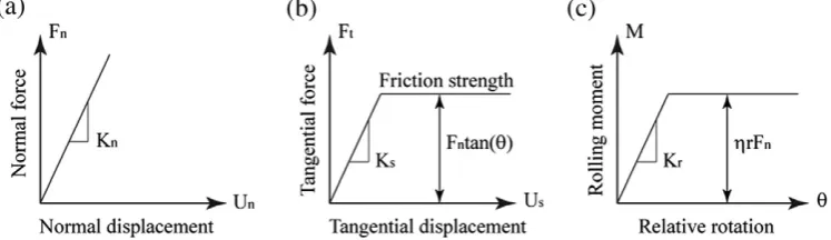
The DEM open source code ESyS-Particle (Weatherley et al., 2011) was employed to run the simulations here presented. Preliminary runs of granular column collapse tests were run employing non-linear elasticity according to the Mindlin no-slip solution (Johnson, 1985) and linear-elastic contacts. No significant difference was found between these analyses. Hence, since linear elastic contacts require less computa-tional time, linear elasticity was adopted. Accordingly, the normal contact force at the contact plane is linearly proportional to the relative normal displacement between two particles (seeFig. 1(a)), expressed as:

Fn¼KnUn ð1Þ

in whichKnis the normal contact stiffness andUnis the normal relative

displacement between two spheres in contact. The response along the tangential direction (seeFig. 1(b)) is calculated incrementally, as:

Fnt ¼F n−1

t þKsdUs ð2Þ

in whichFtnandFtn−1are the tangential forces calculated at the current

and previous simulation time steps;Ksis the shear stiffness, anddUsis

the incremental tangential displacement. The maximum tangential force is limited by the Mohr–Coulomb criterion (seeFigure 1(b)).

A moment–relative rotation law is also present. Here, the rolling law was employed with the only aim of accounting for the shape effect of non-spherical particles. The law accounts for moments arising from the fact that the line of action of the normal contact force in the case of non-spherical particles no longer passes through the centre of mass of the particles and hence generates rotational moments (Belheine

Fig. 1.Particle contact model in DEM (afterBelheine et al. (2009)).

Fig. 2.Particle size distribution of landslides occurred in Northern Apennines (Italy) (after

Casagli et al. (2003)) and rock avalanches in the Alps (Italy) (afterCrosta et al. (2007)). The particle size distribution adopted in the numerical simulations is plotted as the red curve.

Table 1

Parameters of the granularflow simulations.

DEM parameters Value DEM parameters Value

Particle diameter,D(mm) SeeFigure 2 Damping coefficient,α 0.0/0.3 Initial porosity,n 0.43 Coefficient of rolling stiffness,β 1.0 Density,ρ(kg/m3_{) 2650 Coefficient of plastic moment,η 0.1}

Normal stiffness,Kn(N/m) 3 × 107 Simulation parameters Value

Shear stiffness,Ks(N/m) 2.7 × 107 Gravitational acceleration,g(m/s2) −9.81/−981

et al. (2009)). Without this law, unrealistically low angles of repose would be obtained for the granular assembly. In the model adopted, the magnitude of the elastic rolling moment (Me) is proportional to

the relative rotational angle (seeFigure 1(c)), and is calculated in-crementally as:

Mne¼M n−1

e þkrΔθr ð3Þ

whereMenandMen−1are rolling moment values calculated at the

cur-rent and previous simulation time steps;kr=βKsr2is the rolling

stiff-ness, with β being the coefficient of rolling stiffness, rbeing the average particle radius;Δθris the relative rotational angle between

two particles in one iteration step. The maximum rolling moment that can be exchanged is defined as:

Mplastic¼ηrj jFn ð4Þ

in whichηis the so-called coefficient of plastic moment.

The particle size distribution (PSD) is one of the most important fac-tors controlling landslide initiation and soil permeability. The PSD of granularflows varies hugely at different locations (see for instance

Casagli et al. (2003)). In addition, the grain size distribution may vary significantly within the same landslide mass at different depths (Crosta et al., 2007).Fig. 2shows examples of particle size distributions from 7 cases of landslides in the Northern Apennines (Casagli et al., 2003) and 6 cases of rock avalanches in Val Pola in the Alps (Crosta

et al., 2007). It can be observed that the grain size ranges from

0.001 mm to 1000 mm, with a large percentage offine and medium sized grains and a small amount of coarse grains. Large discrepancies can be observed between the various site investigations.

According toFig. 2, grains with diameters ranging from 0.1 to 10 mm were widely observed in different locations. However, in DEM simula-tions, due to computational limitasimula-tions, we used a much narrower par-ticle size distribution with the ratio of maximum to minimum parpar-ticle sizes equal to 2, as shown in the red curve inFig. 2. The input parameters are listed inTable 1.

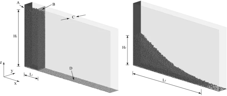
In this study, we carried out numerical experiments of granular columns analogous to the columns of the experimental investigation ofLube et al. (2005). Initially particles were generated within a pris-matic space bounded by two rigid and frictionless walls (A and B in

Figure 3(a)), a rough base (D inFigure 3(a)), and a periodic boundary in the out-of-plane direction (C inFigure 3(a)) to impose plane strain conditions. The horizontal base (D) of the domain (seeFigure 3(a)), is made of particles of the same PSD as the granular column that were keptfixed at all times to simulate a non-erodible base of the same roughness as theflowing material. To generate the granular column,

first particles were randomly created in space (with the grain position allocated according to standard algorithms of random number genera-tion), then they were left to settle under gravity until a dense column was obtained. In all the simulations, the granularflow was initiated by the instantaneous removal of wall B.

Once theflow has stopped, thefinal run-out length (Lf) and deposit

height (Hf) can be measured (seeFigure 3(b)). The presence of single Fig. 3.Model configuration: (a) initial sample; (b)final deposit (A:fixed smooth back wall; B: movable front gate; C: periodic boundary; D:fixed coarsefloor; Li: initial column length; Hi:

initial column height; Lf: runout length; Hf: deposit height).

Table 2

Parameters of the granularflow problem.

Parameter Symbol Unit of measure Independent parameters Initial column length Li [L]

Initial column height Hi [L]

Particle diameter D [L] Particle density ρs [ML−3]

Gravitational acceleration g [LT−2_]

porosity n [–]

Normal stiffness Kn [MT−2]

Shear stiffness Ks [MT−2]

Particle friction angle ϕμ [–]

Coefficient of rolling stiffness β [–] Coefficient of plastic moment η [–] Dependent parameters Final deposit length Lf [L]

Final deposit height Hf [L]

Flow velocity Vf [LT−1]

Granular sliding time t [T]

particles detached from the front of the granular mass sometimes makes the calculation of Lfa non-straightforward exercise. Zenit (2005)calculatesLfconsidering only particles remaining in contact

with each other, disregarding individual loose particles detached from the deposit mass centre. In this study, in order to track the position of the front in a way consistent amongst the various simulations (the number of loose single particles moving ahead of the front depends on the aspect ratio), we implemented an algorithm which identifies the front as the boundary between 99% and 1% of theflow mass, i.e. 1% of the mass is travelling ahead of the boundary. This guarantees that the front is not confused with the position of loose single particles jumping ahead theflow.

3. Dimensional analysis

The physical parameters ruling the motion and the depositional morphology of the granular column include (Zhao et al., 2012): grain properties, geometrical properties of the domain,flow velocity and duration time. InTable 2, all the parameters are listed together with their units expressed in terms of fundamental dimensions, i.e. mass (M), length (L) and time (T). Depending on their role in the simulation, parameters can be categorised as either independent or dependent. We considered the grain properties and the domain

geometry as independent input parameters andfinal runout dis-tance (Lf), deposit height (Hf),flow velocity (vf) andflow duration

time (t) as the dependent ones.

The governing parameters of the mechanical laws ruling particle in-teractions are the normal and shear particle contact stiffness (Kn,Ks),

particle friction (_ϕμ) and the coefficients of rolling resistance (β,η).

Also porosity has a significant influence on the mechanical behaviour of granularflows (Craig, 1997). However, since the primary purpose of this study is to explore the capability of DEM in modelling granular

flows, the influence of porosity has not been considered here. The rela-tionship between the independent and dependent quantities can be expressed by a general functional relationship of the form:

Lf;Hf;vf;t

¼f Li;Hi;D; ρs;g; Kn; Ks;n;ϕμ

ð5Þ

Performing dimensional analysis (Palmer, 2008), and taking out porosity which is the same in all the tests carried out (all columns were generated with the same initial porosity), Eq.(5)can be rewritten as:

L

½ ;_½ H_;½ V_;½ T

ð Þ ¼f a _;ε;½ S_{; ϕμ ð}6_Þ

where [L] = (Lf−Li)/Liis the normalised run-out distance; [H] =Hf/

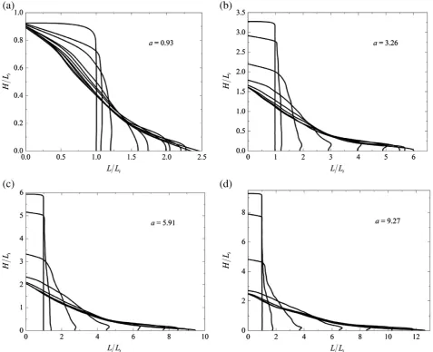
Fig. 5.The evolution of sample profiles for different granular columns (profiles are traced at successive time steps (Δt= ffiffiffiffiffiffiffiffiffiffiHi=g

p

Liis the normalised maximumfinal deposit height;½ ¼V vf=

ffiffiffiffiffiffiffiffi

gHi

p

is the normalisedflow velocity (vfcan be chosen in a variety of ways, one of which is the velocity of propagation of theflow front,i.e. vf=dL/dt);½T ¼t= ffiffiffiffiffiffiffiffiffiffiHi=g

p

is the normalisedflow duration time; a= Hi/Liis the initial column aspect ratio;ε=ρsgHi/(Kn/D) is

a characteristic compressive strain of the granular column and [S] =Hi/Dis the model-to-particle size ratio. Note that [–] indicates

a dimensionless variable.

4. Numerical results

4.1. Calibration of the angle of repose

In studies on non-cohesive granularflows, the material internal fric-tion angle (ϕ) is often approximated by the angle of repose. In simple terms, it can be said that a slope with an angle over the horizontal larger than the angle of repose is unstable, whereas it is stable if the opposite holds true. Typical values for the angle of repose range from 25° for

flows made of smooth spherical particles to 40° for rough angular parti-cles (Carrigy, 1970; Pohlman et al., 2006). Here, we assumed as baseline reference value, an angle of repose of 31° which is representative of coarse quartz sand (Lube et al. (2005)).

With regard to the calibration of the DEM parameters, concerning the rolling stiffness,β, inModenese (2013)it is shown that its influence on the angle of repose is negligible, so it was not investigated here. Then, two contact parameters remain to be determined: the intergranular friction angle,ϕμ, and the coefficient of rolling resistance,η. InZhao (2014), it is shown that some arbitrariness exists since the same angle of repose can be obtained from several combinations of them. Here, we opted to choose an intergranular friction angle ofϕμ= 30°, which

is a typical value for quartz sand grains, and to calibrateηagainst the angle of repose observed when theflow comes to a stop. InFig. 4, the angles of repose obtained for various values ofηare shown. ForηN0, a linear relationship betweenηand the angle of repose exists. For η= 0, an unrealistically low angle of repose is obtained. This is a well-known result reported in Calvetti and Nova (2004), Pöschel and Buchholtz (1993)andRothenburg and Bathurst (1992)). In all the sub-sequent analyses, a value ofη= 0.1, corresponding to an angle of repose for theflow of 31°, was adopted.

4.2. Kinematics of motion

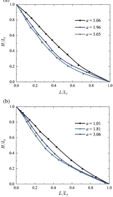
Depending on the initial aspect ratio of the granular column, differ-ent depositional morphologies are obtained (seeFigure 5). As it can be expected, the upper surface of the granularflow gradually lowers until the angle of repose is reached. Our results confirm that theflow profiles at various times and thefinal deposit depend strongly on the initial as-pect ratio (Lube et al., 2005). This highlights the need for presenting profiles in dimensionless form. To this end, thefinal profiles of the gran-ular assembly, normalised by thefinal runout distance and the deposit height, were plotted inFig. 6together with the experimental profiles obtained byLube et al. (2005). The profiles from our 3D DEM analyses exhibit a good agreement with the experimental results for all the as-pect ratios analysed.

A key feature of the DEM is the possibility of obtaining data on the motion of single particles (e.g. trajectories, velocities, etc.) inside the granularflow, allowing performing a detailed analysis of the potential heterogeneities in theflow. For instance, from our analyses, it emerges that in granular columns with small aspect ratios (e.g.a= 0.93), only a small portion of material is involved in the motion. To compare the kinematicfields obtained from columns of different aspect ratios, it is convenient to plot the measured velocities in dimensionless form. To this end, we definepffiffiffiffiffiffiffiffigHias the characteristic velocity of the system. This represents the maximum velocity that a single particle in free-fall from a height corresponding to the centre of the column (Hi/2) reaches

at the end of the fall. InFig. 7(a), particles with velocities smaller than 1% of the characteristic velocity are plotted in grey, whilst particles moving at higher velocities are plotted in red. From thefigure, it can be noted that failure of the granular assembly occurs approximately along a plane, identified by a dashed line in the figure. According to the Rankine's theory of earth pressure (Rankine (1857), assuming that the failure of the granular column occurs when conditions of active thrust are in place, the inclination of the failure plane to the horizontal (θf)

can be estimated as:

θf ¼45∘þϕ=2 ð7Þ

whereϕis the internal friction angle of the granular material. From

Fig. 7(b), it emerges that the inclination angle of the active failure plane is approximately 61° for all the aspect ratios tested. This value is very close to the theoretical value predicted by Eq.(7), which is 60.7°.

4.3. Influence of the column aspect ratio

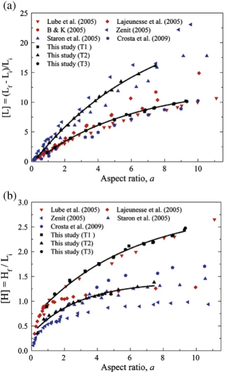
For rock avalanches and granularflows, the assessment of thefinal run-out distance is of primary importance, as it determines the extent

Fig. 6.Final normalised profiles of the granular column deposit: (a) 3D DEM results;

of the regions affected by the avalanche or landslide. InFig. 8(a), our simulations have been compared with previous numerical simulations (Staron and Hinch, 2005; Zenit, 2005; Crosta et al., 2009) and experi-mental observations (Balmforth and Kerswell, 2005; Lajeunesse et al., 2005; Lube et al., 2005) from the literature. We performed three sets of simulations: T1 and T2 refer to simulations run for the same values ofε (ranging from 6.5 × 10−7_{to 6.5 × 10}−6_{), but withη= 0.1 andη= 0} respectively, whilst T3 refers to simulations run forεranging from 6.5 × 10−5_{to 6.5 × 10}−4_{andη= 0.1. Some of the T1 and T2 simulations} were run with gravitational acceleration scaled up 100 times andKn=

3 × 107N/m, whereas some others with unscaled gravity but particles 100 times softer, i.e.Kn= 3 × 105N/m. In fact, in light of dimensional

analysis, scaling can be introduced by scaling either the value of gravita-tional acceleration or particle stiffness. The fact that the obtained results are aligned in consistent trends inFig. 8can be seen as a verification of the correctness of the performed dimensional analysis. Comparison be-tween T1 and T2 simulations allows examining the influence of particle shape on run-out, whereas comparison between T1 and T3 allows exam-ining the influence ofε. The values of the independent variables employed in our simulations are reported inTable 3in terms of the dimensionless groups identified in Eq.(6). In the table, the values of the parameters employed in other tests reported from the literature inFigs. 8 and 9for comparison purposes are listed as well. InFig. 8(a), it can be observed

that thefinal normalised run-out distance obtained from our simulations matches well from a qualitative viewpoint both the experimental obser-vations ofLube et al. (2005)from tests run in plane strain conditions, and the 2D FEM numerical analyses ofCrosta et al. (2009). Also it emerges that if rolling resistance is not employed (simulations T2), unrealistically large run-out distances are obtained since particle angularity tends to re-duce run-out. In other words, aflow of spherical particles is more prone to sliding than aflow of particles of any non-spherical shape. Equally, if 2D DEM simulations are employed (Staron and Hinch, 2005; Zenit, 2005), unrealistically long run outs are obtained. Presumably, this is due to the fact that the 2D kinematics of particle interaction is too different from the real 3D kinematics. Comparison between the simulation series T1 and T3 shows that the characteristic strain of a granular column,ε, has no influence on the observedflow behaviour, at least for the range of values here employed. In conclusion, simulations T1 and T3 show that if particle shape is accounted for, albeit by means of a very crude approxi-mation (i.e. employing a moment–relative rotation law with spherical particles which avoids simulating the real non-spherical geometry of the particles), the obtained run-out andfinal heights of the simulated

flows are in good agreement with the available experimental data. Now let us look at how the front of theflow propagates over time. In

Fig. 9, the position of the front is plotted against time for various column aspect ratios. According to previous literature (Lube et al., 2005; Crosta

et al., 2009), time has been normalised bypffiffiffiffiffiffiffiffiffiffiHi=g, which can be thought of as the time taken by a single particle in free fall to travel from the centre of the column to the base. Looking at thefigure, four typical distinct regimes can be identi_fied: an initial transient acceleration (A), a constant velocityflow (B), a gradual deceleration (C) and afinal static deposition (D). It emerges that in terms of DEM simulations, only 3D

analyses accounting for the effect of particle shape provide results that are in agreement with experiments.

4.4. Analysis of the energy contributions in theflow

The potential energy of the column at any time is:

Ep¼X N

i¼1

mighi ð8Þ

wheremiandhiare the mass and height of a single particlei, respectively,

andNis the total number of particles of the column. The kinetic energy of the system at any time is calculated as:

Ek¼ 1 2

XN

i¼1 mivi

2 þIiωi

2

ð9Þ

where viandωiare the translational and angular velocities respectively of

a generic particlei, andIis its moment of inertia (for a spherical particle I= 2mR2_/5).

A part of potential energy gets dissipated rather than being transformed into kinetic energy, due to unelastic particle collisions (e.g. unelastic particle rebounds and frictional sliding). In light of the principle of energy conservation, the energy dissipated in theflow at any given time can be calculated as:

Ediss¼E0−Ep−Ek ð10Þ

whereE0is the total energy of the system, which can be calculated from

the initial potential energy of the column before particles start to move, as:

E0¼MgHi=2 ð11Þ

whereM¼∑N i¼1

mi.

At the particle level, energy is mainly dissipated via frictional sliding at particle contacts and viscous damping along both the normal and tan-gential directions of contacts when damping is present, but also by the relative rotation between particles once the plastic limit of the rolling moment is reached (seeFigure 1(c)). InFig. 10, the entire temporal evolution of the energy components of theflows, from start of column collapse until end of motion, is plotted. After the instantaneous removal of the confining gate atT= 0, particles start to fall downwards, with po-tential energy being progressively transformed into kinetic energy. The kinetic energy exhibits a peak at aroundT= 1.0 (see the dashed line in thefigure), when both the rate of potential energy loss and the rate of cumulative energy dissipation (see the slopes of the curves in the

figure) reach their maximum values. After this time, both potential and kinetic energy decrease. The_flow comes to a stop at aboutT= 4.0. Considering now columns of different aspect ratios, the dissipated Fig. 8.Relationship between aspect ratio and (a) normalised run-out distance and (b)final

deposit height. The red symbols are experimental results; blue symbols are numerical re-sults, while the numerical results of this study are coloured black.

Table 3

Properties for experimental and numerical tests.

– Test type a ε [S] ϕ(°)

Lube et al. (2005) Experiments in plane strain [0.5, 20] [4.7, 140] × 10−9

[9, 1000] [29.5, 32]

Lajeunesse et al. (2005) Experiments in plane strain [0.2, 12] [1.2, 8.7] × 10−8

[100, 300] [21.5, 22.5]

Balmforth and Kerswell (2005) Experiments in plane strain [0.5, 40] [5.2, 420] × 10−9 _{[12, 1000] [22.5, 26.5]}

Crosta et al. (2009) 2D FEM simulations [0.6, 20] – – [20, 40]

Zenit (2005) 2D DEM simulations [0.1, 10] [2.1, 13.1] × 10−5

[28, 173] 30

Staron (2005) 2D DEM simulations [0.2, 17] – [14, 369] 20

This study (T1)a

3D DEM simulations in plane strain [1, 10] [6.5, 65] × 10−7

[25, 250] 31.7 This study (T2)b

3D DEM simulations in plane strain [1, 10] [6.5, 65] × 10−7

[25, 250] 26.1 This study (T3)a

3D DEM simulations in plane strain [1, 10] [6.5, 65] × 10−5

[25, 250] 31.7

a

Numerical simulation using rolling resistance model (β= 1.0,η= 0.1).

b

energy in terms of percentage of the initial total energy of the columns has been plotted against their aspect ratio inFig. 11. From our simulations, it emerges that the higher the aspect ratio, the larger the proportion of en-ergy dissipated during theflow.

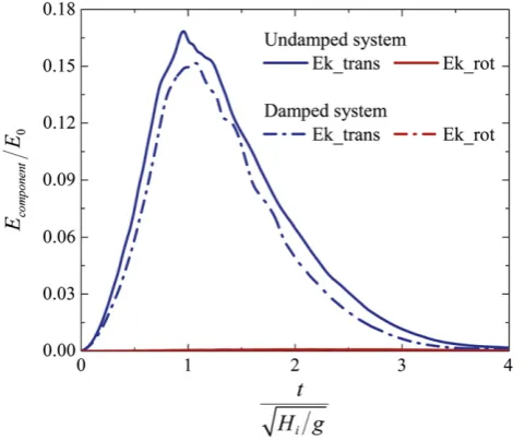
Then, we investigated how much of the kinetic energy of theflow is due to the translation of particles and how much is due to their rota-tions. InFig. 12, the two sources of kinetic energy are plotted separately against time. Unfortunately, viscous damping coefficients strongly de-pend on the type of material making the granularflow. Furthermore, a reliable experimental determination of damping coefficients for granu-larflows is currently not yet available. Therefore, we decided to run two cases only of simulations: one without viscous damping and the other one with a viscous damping coef_ficient of 0.3, in order to obtain a rough indication of the potential influence of viscous damping on the variables of interest but without trying to model any specific natural granular_flow. In the simulations with viscous damping, the damping coefficient of 0.3 was employed in both the normal and tangential direc-tions of particle contacts. This value corresponds to a coefficient of res-titution of around 0.5 (Tsuji et al., 1992). InFig. 12, it can be noted that the kinetic energy stemming from particle rotations remains

negligible at all times (i.e. less than 0.5% of the total kinetic energy) in both cases, with and without the presence of viscous damping. In light of thisfinding, in the next section, where we investigate the spatial dis-tribution of the momentum inside theflow, we have concentrated our attention on the linear momentum since we know the angular momen-tum to be negligible. Also, fromFig. 12, it emerges that the curves ob-tained forflows with and without damping, are similar. This implies that the presence of damping decreases the magnitude of the kinetic energy of the system, of the same proportion, throughout the duration of theflow.

4.5. Linear momentum

The evolution over time of the linear momentum of the_flow,! ¼p

∑N i¼1

mi!vi, is plotted inFig. 13, in the case of the presence of viscous

dissi-pation and in its absence. Given the imposition of periodic boundary conditions in theydirection, we expectpyto be negligible at all times,

as it is shown inFig. 13(a). This confirms the effective presence of plane strain conditions in thex–z plane for the simulated flows.

Fig. 9.Normalized granular spreading length versus normalized time from experimental and numerical tests.

Fig. 10.Variation of energy during granularflow (a = 3.26) (E0: initial total energy; Ep:

normalized potential energy; Ek: normalized kinetic energy; Ediss: normalized cumulative

energy dissipation).

Analogously to the energy analysis of theflow, it is convenient to nor-malise!p, for the sake of generality in presenting our results. To this end, we introduce a scalar quantity,p0, with:

p0≡M ffiffiffiffiffiffiffiffi

gHi

p

ð12Þ

This quantity can be thought of as an approximate average of the momentum of the_flow:p0≡M

ffiffiffiffiffiffiffiffi

gHi

p

¼MHi=

ffiffiffiffiffiffiffiffiffiffi

Hi=g

p

withHi=

ffiffiffiffiffiffiffiffiffiffi

Hi=g

p

being the characteristic velocity of theflow. InFig. 13(a), the compo-nents of the linear momentum along thex,yandzaxes, normalised byp0, are plotted against dimensionless time. A small difference

be-tween the curves for the case with and without damping is noted with damping having the effect of reducing the amount of momentum as it is expected. From thefigure, it emerges that the momentum in the vertical direction,pz, exhibits a higher peak than the momentum

in the direction offlow propagation,px. The two peaks occur at different

times. To better investigate which one is dominant and when, it is con-venient to make a relative comparison between the two components. To this end, the square of each component over the square of the magni-tude of the vector (!p) is plotted inFig. 13(b) and (c). The use of the squares allows for plotting the components as percent, sincepx2

p2 þ py2

p2 þ pz2

p2 ¼100%. From thefigure, it can be noted that at the beginning of theflow, the vertical component,pz, dominates due to the fact that

the motion of the particles is mainly gravity driven free fall. Then, during the propagation phase, the horizontal component,px, becomes

domi-nant, stabilising itself at around 90%. Finally, when theflow is coming to rest, a surge of vertical component appears. This is due to the presence of decelerating particles exhibiting bouncing in the verti-cal direction, especially near the flow forefront. In comparison withFig. 13(b), the start point of the chart inFig. 13(c) looks shifted ahead in time, since it takes some time for theflow front to start moving ahead after gate removal.

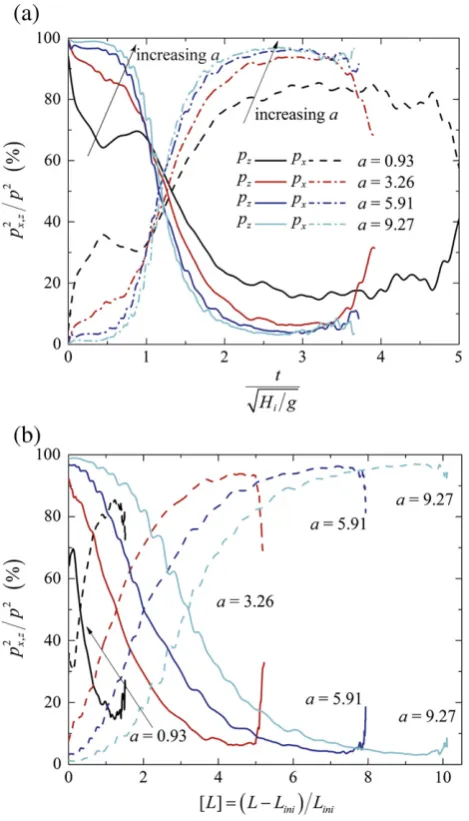
Let us now examine the influence of the column aspect ratio on lin-ear momentum. This is an important aspect in order to ascertain how general the observed trends on the linear momentum of theflow are. InFig. 14, the evolution of the vertical and horizontal components of the linear momentum is plotted (as percentage over the magnitude of the vector!p) against dimensionless time for columns of various aspect ratios. Similar trends amongst the curves can be noted. However, in the initial phase of theflow (forTb1.1), the vertical component of momen-tum increases with the aspect ratio and obviously the opposite is true for the horizontal one. Instead, afterT= 1.1, the vertical component

Fig. 12.Evolution of kinetic energy over time (a = 3.26) (Ek_transand Ek_rotare the

translational and rotational sources respectively of the kinetic energy of the system).

Fig. 13.Evolution of linear momentum over normalised time forflow with and without

damping: a) components of momentum normalised by p0; b) components of momentum

as a percentage of the total momentum against normalised time; c) components of momen-tum as a percentage of the total momenmomen-tum against normalised run-out;xis the direction of

of momentum decreases with the aspect ratio. A possible explanation for the observed aspect ratio dependent trend could be that the gravity driven free fall of particles, which gives rise to the particle vertical mo-tion, increases with the height of the column whereas the friction between particles, which opposes the horizontal motion of the par-ticles, is independent of the column aspect ratio. InFig. 14(b) the components of the momentum are plotted against run-out distance.

4.6. Flux of kinetic energy

To assess the vulnerability of existing structures hit by a granular

flow/avalanche and to design engineering works for the protection of existing structures, two quantities are of interest: energy and momen-tum. The kinetic energy of the particleflow can be seen as an upper bound on the destructive energy that could be unleashed on the struc-ture impacted by theflow. The amount of kinetic energy transferred from theflow to the structure depends on howflow and structure inter-act during the time the structure is impinter-acted by theflow. Hence, the amount of energy released by theflow on the structure is a function of the characteristics of bothflow and structure (for instance the relative

stiffness between the two). Also theflow–structure interaction is likely to change over time, for instance due to the development of irrecover-able (plastic) deformations in the structure. So, it is not possible to pre-dict the transfer of energy (and equally of momentum), unless a specific

flow and a structure of interest are modelled. Here, however, we pro-vide an analysis of the linear momentum and kinetic energy of the

flow, measured at various distances from the initial position of the col-umns, in order to identify an upper bound on the maximum energy that may be imparted to structures knocked by granularflows, under the simplifying assumption of disregarding the effects of any structure– flow interactions.

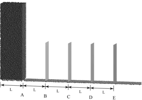
Considering an imaginary vertical section perpendicular to the di-rection of horizontal propagation of theflow (see the vertical plane depicted inFigure 15) theflow mass transiting through such a section is a function of time. This is nil until theflow front reaches the position, then it gradually increases, then decreases and eventually becomes nil again once theflow has come to a stop (seeFigure 15). In the following analysis,five locations along theflow path, shown inFig. 16, are consid-ered. Each location is identi_fied by a letter (seeFigure 16). A convenient measure of the maximum energy that can be transferred from theflow to the impacted structure is what we here call theflux of kinetic energy. This is evaluated as follows: for a given location of interest, the kinetic energy of the particles passing through the vertical plane oriented in the direction perpendicular to theflow is recorded during a specified time intervalΔtand their total kinetic energy,ΔE, is evaluated. The

flux of kinetic energy through the plane is given by the ratio,ΔE/Δt, a quantity with the dimensions of power. It is convenient to normalise this quantity, so that a comparison offluxes between columns of various sizes can be carried out. A simple way of doing so is by normalising both numerator,ΔE, and denominator,Δt. Thus, we define the normalised

flux, P, as:

P≡Δ_EE 0=

Δt

ffiffiffiffiffiffiffiffiffiffi

Hi=g

p ð13Þ

SubstitutingE0from Eq.(11)into Eq.(13)and rearranging, Eq.(13)

can be written as:

P¼Δ_ΔE_t 2 M ffiffiffiffiffiffiffiffiffiffig3_H

i

q ð14Þ

Eq.(14)makes clear that 2 M ffiffiffiffiffiffiffig3_H

i

p is the multiplying factor to normalise

the measuredfluxΔE/Δt. Theflux,P, represents the maximum energy that can be transferred from theflow to the impacted structure. In fact, if all the energy were to be transferred away from theflow, the

flow would be suddenly deprived of all its kinetic energy and therefore it would come to a stop, which is evidently an unrealistic scenario. In re-ality, only a portion of the energy of theflow is lost in the interaction with the structure that will cause theflow to slow down but not to stop. So,Pcan be thought of, as an upper bound on the maximum de-structive power that theflow may impart on the impacted structure. InFig. 17(a), theflux of kinetic energy at the selected locations is plotted versus dimensionless time. It can be noted that the section with highest

flux is B. Obviously thefluxes in the case damping is present are smaller than the case of undampedflow. An interestingfinding is the fact that the peak takes place at a different time, with the time of peak for the damped system shifting progressively ahead of the peak time for the undamped one. Also, the difference of value between the peaks for the damped and undamped systems increases with the distance of the sec-tion investigated from the column initial posisec-tion reaching up to 50% of the peak value for the undamped system.Fig. 17(b) illustrates the evo-lution of the height of the granular mass at different locations. From the

figure, it can be concluded that the further the location is away from the slope source region, the lower the height of thefinal granular mass is.

Fig. 14.Evolution of linear momentum over time for various aspect ratios (with viscous

Fig. 18illustrates the evolution of theflux of kinetic energy for differ-ent column aspect ratios. From thefigure, it can be observed that the po-sition of the section where theflux is highest depends on the aspect ratio. For instance, in the case of small aspect ratios (e.g.a= 0.93), theflux of destructive energy at location A is largest, with only a small amount of particles travelling to locations further down section B. For intermediate aspect ratios (e.g.a= 3.26, 5.91), the largestflux takes place at location B. For large aspect ratios (e.g.a= 9.27), the largest

flux occurs again at section A.

4.7. Distribution offlux of kinetic energy and linear momentum over depth

To be able to design protective structures as effectively as possible, the spatial distributions of kinetic energy and momentum over the depth of the considered sections are also needed. Considering section B, we have split the depth of theflow,h(t), into 5 parts and calculated theflux of kinetic energy through the section for each part so as to obtain a vertical profile of theflux of kinetic energy (seeFigure 19(a)). Looking at thefigure, it emerges that the profile of theflux is initially

Fig. 15.Schematic view of granularflows past a structure.

Fig. 16.Location of the sections where the granularflow is measured along the granular

flow path.

bilinear, with the maximum_flux at middle height of the column, then theflux evolves into a linear profile whose amplitude progressively reduces over time until becoming nil. The bilinear distribution points out to the presence of an uppermost layer of particles in an agitated loose state, which, after some time, consolidates so that a linear distri-bution is obtained. The presence of this layer of loose material is confirmed by the calculation of the profile of mass rate normalised by the totalflow mass in the section (seeFigure 19(c)).

A convenient measure of the maximum momentum that could be transferred by theflow to the impacted structure is theflux of linear momentum over time. Analogously to theflux of kinetic energy, we can evaluate the linear momentum of the particles passing through the vertical section of interest,Δp, during a specified time intervalΔt. Theflux of linear momentum through the whole section or parts of it, is given byΔp/Δt, a quantity with the dimensions of force (so we call itF). It is convenient to normalise this quantity so that comparison of

fluxes between columns of various sizes can be carried out. A simple way of doing this is by normalising both numerator and denominator. So, we define the normalised linear momentum of theflow in the unit of time as:

Fx_;y;z≡ Δpx;y;z

p0 =

Δt

ffiffiffiffiffiffiffiffiffiffi

Hi=g

p ð15Þ

withp0being an average linear momentum for theflow here defined in

Eq.(12). Substitutingp0from Eq.(12)and rearranging, Eq.(15)can also be written as:

Fx_;y;z¼ Δpx;y;z

Δt 1

Mg ð16Þ

Eq.(16)makes clear that 1/Mgis the multiplying factor to normalise the momentum going through the plane in the unit of time. In terms of the value of theflux of the momentum at various sections in time, similar

figures as those obtained for theflux of kinetic energy (Figures 17 and 18) are obtained which are not reported here for sake of brevity. To lo-cate critical sections and times of interest one of the twofluxes, either theflux of kinetic energy or of momentum, is enough. However, it is of interest to practitioners appointed with designing engineering works for the mitigation of theflow hazard, to know the value of the

flux of momentum over depth in order to have an idea of the distribu-tion of the pressure that can act on the structure. InFig. 19(b), the dis-tribution of the horizontal component of the linear momentum along the direction offlow propagation,Fx, over depth is plotted against

time. As it can be expected, the same shape of the profile as the profile of theflux of kinetic energy is found.

5. Conclusions

This paper presents a numerical investigation of the behaviour of dry granularflows generated by the collapse of prismatic columns via 3D Distinct Element Method (DEM) simulations under plane strain conditions. This type of analysis showcases the potential of the Distinct Element Method to investigate the phenomenology of dry granular

flows and to gather unique information currently unachievable by exper-imentation. By means of dimensional analysis, the governing parameters of the problem were identified. Then, the influence of key variables of the problem was analysed. The main results are summarised as below:

(1) Different regimes of granular motion have been observed, de-pending on the initial aspect ratios. The DEM results qualitatively match the FEM analyses byCrosta et al. (2009)and the experi-mental results byLube et al. (2005). The granular material slides along a plane which approximately corresponds to the active failure plane of the column in agreement with Rankine's theory. (2) Quantitative relationships between the column aspect ratio and normalised runout distance and deposit height were established. Using the rolling resistance model, i.e. assigning a moment–

relative rotation contact law, the DEM simulations give rise to runout distances and deposit height which match well the avail-able numerical and experimental results.

(3) A detailed analysis of how energy is dissipated by granular_flows was performed from which emerges that most of the energy of the columns is dissipated by inter-particle friction, with frictional dissipation increasing with the column aspect ratio. Also, the translational and rotational components of the kinetic energy of theflows, associated to particle rotational and translational mo-tions respectively, were monitored during the simulamo-tions. It is found that the rotational component is negligible in comparison with the translational one; hence in order to calculate the de-structive power of a granularflow slide, only the translational contribution of the kinetic energy is relevant.

(4) A methodology is presented to calculate theflux of kinetic energy over time carried by the granularflow through any vertical sec-tion of interest. This can be related to the energy released by landslide induced granularflows impacting against engineering structures under the simplifying assumption of neglecting all structure_–flow interactions. This represents the_first step to-wards achieving a computational tool quantitatively predicting the destructive power of a givenflow at any location of interest along its path. This could be useful for the design of engineering works for natural hazard mitigation. To this end, also the distri-bution of the linear momentum of theflow over depth was calcu-lated. It emerges that the distribution is initially bilinear, due to the presence of an uppermost layer of particles in an agitated loose state, but after some time becomes linear.

Acknowledgements

The second author has been supported by Marie Curie Actions-International Research Staff Exchange Scheme (IRSES): GEO-geohazards and geomechanics, Grant No. 294976.

References

Balmforth, N.J., Kerswell, R.R., 2005.Granular collapse in two dimensions. J. Fluid Mech. 538, 399–428.

Belheine, N., Plassiard, J.P., Donzé, F.V., Darve, F., Seridi, A., 2009.Numerical simulation of drained triaxial test using 3D discrete element modeling. Comput. Geotech. 36, 320–331.

Calvetti, F., Nova, R., 2004.Micromechanical approach to slope stability analysis. In: Darve, F., Vardoulakis, I. (Eds.), Degradations and Instabilities in Geomaterials. Springer, Vi-enna, pp. 235–254.

Fig. 19.Profile of kinetic energy, momentum and mass trough plane B at different times

(a = 3.26). (a) Profile of kinetic energyflux (b) Profile of normalised momentum. (Δpx

Carrara, A., Crosta, G., Frattini, P., 2008. Comparing models of debris-flow susceptibility in the alpine environment. Geomorphology 94, 353–378.http://dx.doi.org/10.1016/j. geomorph.2006.10.033.

Carrigy, M.A., 1970. Experiments on the angles of repose of granular materials. Sedimen-tology 14, 147–158.http://dx.doi.org/10.1111/j.1365-3091.1970.tb00189.x. Casagli, N., Ermini, L., Rosati, G., 2003. Determining grain size distribution of the material

composing landslide dams in the Northern Apennines: sampling and processing methods. Eng. Geol. 69, 83–97.http://dx.doi.org/10.1016/s0013-7952(02)00249-1. Cleary, P.W., Campbell, C.S., 1993.Self-lubrication for long runout landslides: examination

by computer simulation. J. Geophys. Res. Solid Earth 98, 21911–21924.

Collins, G.S., Melosh, H.J., 2003. Acousticfluidization and the extraordinary mobility of sturzstroms. J. Geophys. Res. Solid Earth 108, 1–14.http://dx.doi.org/10.1029/ 2003jb002465.

Craig, R.F., 1997.Soil mechanics. E & FN SPON, London and New York.

Crosta, G.B., Imposimato, S., Roddeman, D., Chiesa, S., Moia, F., 2005. Small fast-movingfl ow-like landslides in volcanic deposits: the 2001 Las Colinas Landslide (El Salvador). Eng. Geol. 79, 185–214.http://dx.doi.org/10.1016/j.enggeo.2005.01.014.

Crosta, G.B., Frattini, P., Fusi, N., 2007. Fragmentation in the Val Pola rock avalanche, Italian Alps. J. Geophys. Res. Earth Surf. 112.http://dx.doi.org/10.1029/2005jf000455F01006. Crosta, G.B., Imposimato, S., Roddeman, D., 2009. Numerical modeling of 2-D granular

step collapse on erodible and nonerodible surface. J. Geophys. Res. Earth Surf. 114, 1–19.http://dx.doi.org/10.1029/2008jf001186.

Cundall, P.A., Strack, O.D.L., 1979.A discrete numerical model for granular assemblies. Geotechnique 29, 47–65 (doi: citeulike-article-id:8653064).

De Blasio, F.V., Elverhøi, A., 2008.A model for frictional melt production beneath large rock avalanches. J. Geophys. Res. Earth Surf. 113 F02014.

Goren, L., Aharonov, E., 2007. Long runout landslides: the role of frictional heating and hydraulic diffusivity. Geophys. Res. Lett. 34.http://dx.doi.org/10.1029/2006gl028895

L07301.

Hungr, O., Evans, S.G., 2004.Entrainment of debris in rock avalanches: an analysis of a long run-out mechanism. Geol. Soc. Am. Bull. 116, 1240–1252.

Iverson, R.M., 1997.The physics of debrisflows. Rev. Geophys. 35, 245–296.

Iverson, R.M., Reid, M.E., Logan, M., LaHusen, R.G., Godt, J.W., Griswold, J.P., 2011.Positive feedback and momentum growth during debris-flow entrainment of wet bed sediment. Nat. Geosci. 4, 116–121.

Johnson, K.L., 1985.Contact Mechanics. Cambridge University Press, Cambridge.

Kerswell, R.R., 2005.Dam break with Coulomb friction: a model for granular slumping? Phys. Fluids 17, 1–16.

Lacaze, L., Phillips, J.C., Kerswell, R.R., 2008.Planar collapse of a granular column: experi-ments and discrete element simulations. Phys. Fluids 20, 1–12.

Lajeunesse, E., Monnier, J.B., Homsy, G.M., 2005.Granular slumping on a horizontal sur-face. Phys. Fluids 17, 1–15.

Linares-Guerrero, E., Goujon, C., Zenit, R., 2007.Increased mobility of bidisperse granular avalanches. J. Fluid Mech. 593, 475–504.

Lube, G., Huppert, H.E., Sparks, R.S., Freundt, A., 2005.Collapses of two-dimensional gran-ular columns. Phys. Rev. E. 72, 1–10.

Mangeney, A., Bouchut, F., Thomas, N., Vilotte, J.P., Bristeau, M.O., 2007.Numerical model-ing of self-channelmodel-ing granularflows and of their levee-channel deposits. J. Geophys. Res. 112.

Mangeney, A., Roche, O., Hungr, O., Mangold, N., Faccanoni, G., Lucas, A., 2010. Erosion and mobility in granular collapse over sloping beds. J. Geophys. Res. Earth Surf. 115.

http://dx.doi.org/10.1029/2009jf001462F03040.

Melosh, H.J., 1979. Acousticfluidization: a new geologic process? J. Geophys. Res. Solid Earth 84, 7513–7520.http://dx.doi.org/10.1029/JB084iB13p07513.

Modenese, C., 2013.Numerical Study of the Mechanical Properties of Lunar Soil by the Discrete Element Method. DPhil, University of Oxford (D.Phil Thesis).

Palmer, A.C., 2008.Dimensional Analysis and Intelligent Experimentation. World Scientific.

Phillips, J.C., Hogg, A.J., Kerswell, R.R., Thomas, N.H., 2006.Enhanced mobility of granular mixtures offine and coarse particles. Earth Planet. Sci. Lett. 246, 466–480.

Pohlman, N.A., Severson, B.L., Ottino, J.M., Lueptow, R.M., 2006.Surface roughness effects in granular matter: influence on angle of repose and the absence of segregation. Phys. Rev. E. 73, 031304.

Pöschel, T., Buchholtz, V.V., 1993.Static friction phenomena in granular materials: Coulomb law versus particle geometry. Phys. Rev. Lett. 71, 3963–3966.

Rankine, W.J.M., 1857. On the stability of loose earth. Philos. Trans. R. Soc. Lond. 147, 9–27.http://dx.doi.org/10.2307/108608.

Roche, O., Attali, M., Mangeney, A., Lucas, A., 2011. On the run-out distance of geophysical gravitationalflows: insight fromfluidized granular collapse experiments. Earth Planet. Sci. Lett. 311, 375–385.http://dx.doi.org/10.1016/j.epsl.2011.09.023.

Rothenburg, L., Bathurst, R.J., 1992.Micromechanical features of granular assemblies with planar elliptical particles. Geotechnique 42, 79–95.

Saucedo, R., Macías, J.L., Sheridan, M.F., Bursik, M.I., Komorowski, J.C., 2005.Modeling of pyroclasticflows of Colima Volcano, Mexico: implications for hazard assessment. J. Volcanol. Geotherm. Res. 139, 103–115.

Shreve, R.L., 1968.Leakage andfluidization in air-layer lubricated avalanches. Geol. Soc. Am. Bull. 79, 653–658.

Staron, L., Hinch, E.J., 2005.Study of the collapse of granular columns using DEM numer-ical simulation. J. Fluid Mech. 545, 1–27.

Staron, L., Hinch, E., 2007. The spreading of a granular mass: role of grain properties and initial conditions. Granul. Matter 9, 205–217. http://dx.doi.org/10.1007/s10035-006-0033-z.

Tang, C.L., Hu, J.C., Lin, M.L., Angelier, J., Lu, C.Y., Chan, Y.C., Chu, H.T., 2009. The Tsaoling landslide triggered by the Chi-Chi earthquake, Taiwan: insights from a discrete element simulation. Eng. Geol. 106, 1–19.http://dx.doi.org/10.1016/j.enggeo.2009. 02.011.

Tsuji, Y., Tanaka, T., Ishida, T., 1992.Lagrangian numerical-simulation of plugflow of cohesionless particles in a horizontal pipe. Powder Technol. 71, 239–250.

Utili, S., Crosta, G.B., 2011a. Modelling the evolution of natural slopes subject to weathering: Part I. Limit analysis approach. J. Geophys. Res. Earth Surf. 116, F01016.

http://dx.doi.org/10.1029/2009JF001557.

Utili, S., Crosta, G.B., 2011b. Modelling the evolution of natural slopes subject to weathering: Part II. Discrete element approach. J. Geophys. Res. Earth Surf. 116, F01017.http://dx.doi.org/10.1029/2009JF001559.

Utili, S., Nova, R., 2008.DEM analysis of bonded granular geomaterials. Int. J. Numer. Anal. Methods Geomech. 32 (17), 1997–2031.

Weatherley, D., Boros, V., Hancock, W., 2011.ESyS-Particle Tutorial and User's Guide Version 2.1. Earth Systems Science Computational Centre, The University of Queensland.

Zenit, R., 2005.Computer simulations of the collapse of a granular column. Phys. Fluids 17, 1–4.

Zhao, T., 2014.Investigation of Landslide-Induced Debris Flows by the DEM and CFD. DPhil, University of Oxford (D.Phil Thesis).