Dynamic Modelling with a Modified PID Controller of a Three Link Rigid Manipulator

(1)

Dynamic Modelling with a Modified PID Controller of a

Three Link Rigid Manipulator

Sherif G. Ahmad

Faculty of Engineering,

Mansura University,

Egypt

Ahmad S. Elbanna

Air Defense R & D,

Cairo, Egypt

Mohamad S. Elksas

Assistant Professor at

Computers & Systems

Engineering, Mansoura

University, Egypt

Fayez G. Areed

Professor at Computers

and

Systems Engineering,

Mansoura University,

Egypt

ABSTRACT

This paper presents the modelling of three links rigid manipulator (TRLM) deriving its dynamic equations depending on Lagrange/Euler (L-E) method, the manipulator design and implementation has a complexity, uncertainty and instability dynamic features which lead to a non-linear characteristics, so controlling the manipulator means controlling multi-body multi-input multi-output (MIMO) non-linear and coupled system, the second part of this paper introduce a precise modified Proportional Integral Derivative (PID) controller to control the manipulator under applying different scenarios for the reference signal according to manipulator applications.

Keywords

Dynamic modelling, Three link rigid manipulator, Lagrange-Euler, PID controller, Differential evolution

1. INTRODUCTION

Recently robots have been considered as an indispensable part of advanced manufacturing field with the ability of robots to accomplish hazardous and risky jobs for human. In robotics, there are two main subjects which are kinematics and dynamics. Within the science of kinematics one studies the position, the velocity, the acceleration and all higher order derivatives of the position variables. Kinematics itself is divided into Forward and Inverse kinematics [1, 2].

However, the relationship between these motions and the forces and torques that cause them constitutes the problem of dynamics [3, 4]. The dynamic model of a robot studies the relation between the joint actuator torques and the resulting motion.

There are two problems related to the dynamics of a manipulator; the first; given the trajectory point [position (𝜃), velocity (𝜃 ), and acceleration (Ӫ)] and we wish to calculate the required vector of joint torques (𝜏). In other words, computation of the vector 𝜏(𝑡) necessary to obtain a desired trajectory 𝑞 (t), 𝑞 (t), q(t) (q is the generalized joint coordinates), once the forces applied of the end-effector are known. This is the Inverse dynamic problem.

The second is to calculate how the mechanism will move under application of a set of joint torques, that is, given a torque vector 𝜏 calculate the resulting motion (position, velocity, acceleration) of the manipulator In other words, computation of the time evolution of 𝑞 (t) then of 𝑞 (t) and q(t), given the vector of generalized forces (torques) 𝜏(𝑡) applied to the joints and, in case, the external forces applied to the end-effector, and the initial conditions q(t = t0) 𝑞 (t = t0) and

this is Direct dynamic model [5]. An accurate dynamic model of a robot manipulator has many benefits; for the design of motion control system, analysis of mechanical design, and simulation of manipulator motion [6]. In other words, to achieve a proper control, a valid dynamic model must be obtained. In Kostic et al. [7] approach for modeling and identification of a high-performance robot control, they highlighted a procedure for obtaining kinematic and dynamic models of a robot for the control design. The procedure involves deduction of the robot’s kinematic and dynamic models, estimation of the model parameters experimentally, validation of the model and identification of the remaining robot dynamics, which should not be ignored if robustness and high-performance robot operation are required. There are many approaches for generating the dynamic equations of a mechanical system.

Two commonly methods are used for formulating the dynamics based on the specific geometric and inertial parameters of the robot, they are L-E formulation and the recursive Newton-Euler method [8]. Both are equivalent as both describe the dynamic behaviour of the robot motion, but are specifically useful for different purposes. We will use L-E method for our derivation which relies on the energy properties of mechanical systems to compute the equations of motion.

Serial linkage robot arms are a highly non-linear uncertain system with complicated interactions between each joint [9]. These interactions represent gravitational forces dependent on the position of the joint, effective inertia forces due to the acceleration of each joint where the deriving torque is acting reaction forces due to the accelerations of other joints, Coriolis forces generated by the velocities of the other joints and centrifugal forces generated by the angular velocity of each joint. Therefore, the robot arms are usually assumed as non-linear, uncertain, MIMO system.

The most used form of industrial controllers is the PID controller. Statistics shows that they constitute more than 90% of feedback controller used today. This is because it’s low cost, simple in structure and robust in performance over a wide range of operation conditions [10].

(2)

2. DYNAMICS OF THREE-LINKS

MANIPULATOR

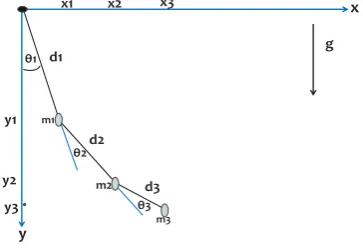
We consider the three-link robotic manipulator. The physical system is shown in fig. 1

Fig.1 Three Link Manipulator

The system consists of three masses connected by weightless bars. The bars have length d1, d2, d3. The masses are denoted by m1, m2, m3, respectively.

Let 𝜃1, 𝜃2, 𝜃3 denote the angles in which the first bar rotates about the origin and the second bar rotates about endpoint of the first bar.

The equations for the x-position and the y-position: X1 = d1 sin 𝜃1, Y1 = - d1 cos 𝜃1 (1) X2 = d1 sin 𝜃1 + d2 sin (𝜃1 + 𝜃2),

Y2 = - [d1 cos 𝜃1+d2 cos (𝜃1+𝜃2)] (2) X3 = d1 sin 𝜃1 + d2 sin (𝜃1 + 𝜃2) + d3 sin (𝜃1 + 𝜃2 +𝜃3)

Y3 = - [d1 cos 𝜃1 + d2 cos (𝜃1+𝜃2) + d3 cos (𝜃1+𝜃2+𝜃3)] (3)

The joint velocity of each link,

V12 = 𝑥 12+𝑦 12, V22 = 𝑥 22+𝑦 22, V32 = 𝑥 32+𝑦 32 (4) The Kinetic energy (K.E) of each link,

K

i

= ½ m

i

v

i2

(5)

i = 1, 2, 3 (no. of joints) The total K.E of all links;

K = K

1

+ K

2

+ K

3

(6)

The potential energy (P.E) of each link;

P

i

= - m

i

g Y

i

(7)

The total P.E of all links;

P = P

1

+ P

2

+ P

3

(8)

2.1 Lagrange-Euler Formulation

The L-E equations are obtained as [2]:

L = K – P

,

𝜏

i

= d/dt [

𝛿

L /

𝛿𝜃

i

] –

[𝛿𝐿

/

𝛿𝜃

i

]

(9)

Where:

K = Total kinetic energy of the robot arms system. P = Total potential energy of the robot arms system

𝜃i = Generalized coordinates of the robot arms.

𝜃 i = First time derivative of the generalized coordinate.

𝜏i = Generalized torques applied to the system at joint i

to drive link i.

By applying (9) to The Lagrange function of the robot arm yields the necessary generalized torque Ti for joint i actuator to drive the i-th link of the manipulator, for i = 1, 2, 3 which gives:

𝜏₁ = [(m₁ + m₂ + m₃) d₁₂ + (m₂ + m₃) d₂₂

+ m3 d32+ 2 (m2 + m3) d1 d2 cos 𝜃2+2 m3

d2 d3 cos 𝜃3+ 2 m3 d1 d2 cos (𝜃2 +

𝜃3)] Ӫ 1+[(m1+ m2) d22+ m3d32 + (m2+m3) d1 d2

cos𝜃₂ + 2 m₃ d₂ d₃ cos𝜃₃ + m₃ d₁ d₂

cos(𝜃₂+𝜃₃)] Ӫ₂_{+ [m}₃_d₃₂_+m₃_d₂_d₃_cos𝜃₃+m₃d₁

d2 d3 cos (𝜃2+𝜃3)] Ӫ3 - [(m2 + m3) d1 d2 sin

𝜃₂+ m₃ d₁ d₂ sin (𝜃₂ + 𝜃₃)] 𝜃 ₂₂ - [m₃ d₂ d₃

sin 𝜃₃ + m₃ d₁ d₂ sin (𝜃₂ + 𝜃₃)] 𝜃 ₃₂ -[2

(m2 + m3) d1 d2 sin 𝜃2 + 2 m3 d1 d2 sin

( 𝜃₂ + 𝜃₃)] 𝜃 ₁ 𝜃 ₂ - [2 m₃ d₂ d₃ sin 𝜃₃ + 2

m3 d1 d2 sin (𝜃2 + 𝜃3)] 𝜃 1 𝜃 3 - [2 m3 d2

d3 sin 𝜃3 + 2 m3 d1 d2 sin (𝜃2 + 𝜃3)] 𝜃 2

𝜃 ₃ + [(m₁ + m₂ + m₃) d₁ g sin 𝜃₁+ (m₂ +

m3) d2 g sin (𝜃2 + 𝜃1)+ m3 d3 g sin ( 𝜃1 +

𝜃₂ + 𝜃₃) (10)

𝜏

₂_{= [(m}₁_{+ m}₂_{) d}₂₂_{+ m}₃_d₃₂_{+ (m}₂_{+ m}₃₎

d1 d2 cos 𝜃2+ 2 m3

d2 d3 cos 𝜃3 + m3 d1 d2 cos (𝜃1 + 𝜃3)]

Ӫ₁_{+ [(m}₂_{+ m}₃_{) d}₂₂_{+ m}₃_d₃₂_{+ 2 m}₃_d₁_d₂

cos 𝜃₃] Ӫ₂_{+ [m}₃_d₃₂_{+ m}₃_d₂_d₃_cos𝜃₃]

Ӫ₃_{+ [(m}₂_{+ m}₃_{) d}₁_d₂_sin𝜃₂ + m₃ d₁ d₂

sin (𝜃₂ + 𝜃₃)] 𝜃 ₁₂ - [m₂ d₂ d₃ sin 𝜃₃] 𝜃 ₃₂ -

[2 m3 d2 d3 sin 𝜃3] 𝜃 1 𝜃 3 - [2 m3 d1 d2

sin 𝜃₃] 𝜃 ₂ 𝜃 ₃+ [(m₂ + m₃) d₁ g sin (𝜃₁ +

𝜃₂) + m₃ d₃ g sin (𝜃₁ + 𝜃₂ +𝜃₃)]

(11)

𝜏

₃_{= [m}₃_{+ d}₃₂_{+ m}₃_d₂_d₃_cos𝜃₃ + m₃ d₁

d2 cos (𝜃2 + 𝜃3)]

Ӫ₁_{+ [m}₃_d₃₂_{+ m}₃_d₂_d₃_cos𝜃₃] Ӫ₂_{+ m}₃ d32 Ӫ3+ [m3 d2 d3 sin 𝜃3 + m3 d1 d2 sin

(𝜃₂ + 𝜃₃)] 𝜃 ₁₂ + [m₃ d₁ d₂ sin 𝜃₃] 𝜃 ₂₂ - [2

m3 d2 d3 sin 𝜃3] 𝜃 1 𝜃 2 + m3 d3 g sin

( 𝜃+𝜃₂+ 𝜃₃) (12)

Let us rewrite the dynamic equations in the general form:

𝜏

i

=D

ii

𝜃

i

"Effective torque''

+D

ik

𝜃

k

+D

im

𝜃

m

"Coupling torque"

+D

iii

𝜃

i2

+D

ikk

𝜃

k2

+D

imm

𝜃

m2

"Centrifugal torque"

+ D

iik

𝜃

i

𝜃

k

+ D

iki

𝜃

k

𝜃

i

+D

iim

𝜃

i

𝜃

m+D

imi

𝜃

m

𝜃

i

"Coriolis torque"

+

D

ikm

𝜃

k

𝜃

m

+

D

imk

𝜃

m

𝜃

k

+D

i

"Gravity torque"

x

y

d1

d2 x1 x2

y1

y2 m2 _d3

θ1

θ2

Fig. (1) Three links robot manipulator

g x3

θ3

y3 m1

[image:2.595.76.258.132.257.2]

(3)

Unfortunately, the computation of these coefficients requires a large amount of arithmetic operations. Thus, the L-E equations are very difficult to utilize for real-time control purposes unless they are simplified [11].

These dynamic motion equations of a manipulator are coupled, nonlinear, and second order ordinary differential equations. The use of these equations to compute the joints torques from the given joint positions, velocities and accelerations for each trajectory set point in real time has been a computational bottleneck. In order to perform real-time control, a simplified robot arm dynamic model is proposed which ignores the Coriolis and centrifugal forces [12].

2.2 State Space Representation

The derivation of the dynamic model of a manipulator based on the L-E formulation is simple and systematic. The L-E equations of motion can be utilized to solve for the forward dynamics problem.

Next, we transform the dynamic equations (second order differential equation) into the state space representation [13]. The coupling inertias are neglected since they are very small compared with the effective joint inertia. It is noted that, the design of the variable structure controller does not require accurate mathematical dynamic model of the manipulator, thus the bounds of the model parameters are sufficient to construct the controller. This property is desirable since the complexity of the manipulator dynamics make the exact calculation of the dynamics infeasible if not impossible [5, 11].

Define the state variables as:

𝜃

1

= x

1

,

𝜃

1

= x

2

𝜃

2

= x

3

,

𝜃

2

= x

4

𝜃

3

= x

5

,

𝜃

3

= x

6

𝜃

1

=

𝑥

1

= x

2

Ӫ

1

=

𝑥

2

= [

𝜏

1

+D

122

x

42

+D

133

x

62

+D

112

x

2

x

4

+D

113

x

2

x

6

+D

123

x

4

x

6

–C

1

] / D

11

𝜃

2

=

𝑥

3

= x

4

Ӫ

2

=

𝑥

4

= [

𝜏

2

+ D

233

x

62

+ D

231

x

2

x

6

+ D

223

x

4

x

6

– D

211

x

22

– C

2

] / D

22

𝜃

3

=

𝑥

5

= x

6

Ӫ

3

=

𝑥

6

= [

𝜏

3

+ D

311

x

22

+ D

322

x

42

+ D

312

x

2

x

4

– C

3

] /

D

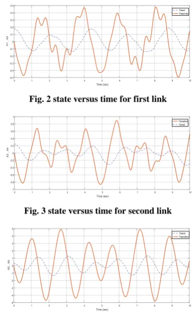
33

By applying Rung-Kutta forth order (ode-45) method with a sample rate (0.001) to solve the above equations, assuming the following parameters,

m1 = 1 kg, m2 = 0.8 kg, m3 = 3 kg, d1 = 1 m, d2 = 0.8 m, d3 = 0.6 m With initial conditions:

x (0) = [0.175, 0, 0.25, 0, 0.275, 0]

T

,

The torques 𝜏i are set to Zero,

[image:3.595.331.523.73.387.2]

That is there is no control on the links. These leads to the results shown in the figures 2, 3 and 4 below:

Fig. 2 state versus time for first link

Fig. 3 state versus time for second link

Fig. 4 State versus time for third link

As shown in the above figures, the system performance is oscillatory under no torques applied (without control). The velocity of the link decreases as it goes to the point of changing direction till it becomes zero at the point of changing direction then, it starts to increase again.

In general, the motion control problem consists of obtaining dynamic model of the manipulator and validates this model, then using this model to design a robust controller that achieves the desired response and performance that resists the environmental characteristics.

3 CONTROLLER DESIGN

The control problem for robot manipulators is the problem of determining the time history of joint inputs required to hold the system of three links in a particular position on X-Y plane or to cause the end-effector to execute a command motion. Having a robust controller gives us the ability to hold each link at a particular angle 𝜃i with respect to X-axis. Our algorithm used works by defining an error variable which is the difference between the desired position (target position) and the real position of the manipulator with the effect of the controller.

The general form of equations of motion can be written as

𝜏 = M (𝑞)𝑞 + V (𝑞, 𝑞 ) + G (𝑞)

(13)

Where, q is the generalized joint coordinates M (𝑞) is the mass matrix (inertia matrix) V (𝑞,𝑞 ) is the centrifugal & Coriolis forces G (𝑞) is the gravity forces

(4)

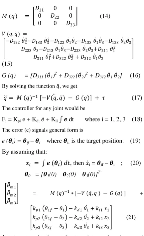
𝑀 (𝑞) =

𝐷

11

0

0 𝐷

₂₂

0

0 𝐷

₃₃

(14)

𝑉 (𝑞, 𝑞 ) =

−𝐷122 𝜃 22−𝐷133 𝜃 32−𝐷122 𝜃 1𝜃 2−𝐷133 𝜃 1𝜃 3−𝐷123 𝜃 2𝜃 3 𝐷233 𝜃 3−𝐷213 𝜃 1𝜃 3−𝐷223 𝜃 2𝜃 3+𝐷211 𝜃 12

𝐷311 𝜃 12+𝐷322 𝜃 22+ 𝐷312 𝜃 1𝜃 2

(15)

G (

𝑞

) = [D

311

(

𝜃

1

)

2

+ D

322

(

𝜃

2

)

2

+ D

312

𝜃

1

𝜃

2

]

(16)

By solving the function 𝑞 , we get

𝑞 = 𝑀 (𝑞)

−1

_{[−𝑉(𝑞, 𝑞 ) − 𝐺 (𝑞)] + 𝜏}

₍₁₇₎

The controller for any joint would be

F

i

= K

pi

e + K

di

𝑒

+ K

ii

𝒆

dt where i = 1, 2, 3 (18)

The error (e) signals general form is

e (

𝜽

i

) =

𝜽

if

–

𝜽

i

where

𝜽

if

is the target position. (19)

By assuming that:

𝑥

_𝑖

= 𝒆 (𝜽

𝒊

) 𝑑𝑡

, then

𝑥

i

=

𝜽

if

–

𝜽

i

; (20)

𝜽

0

= [

𝜽

1

(0)

𝜽

2

(0)

𝜽

3

(0)]

T

𝜃 𝑚1 𝜃 𝑚2 𝜃 𝑚3

= 𝑀 (𝑞)−1_{∗ [−𝑉 (𝑞 , 𝑞 ) − 𝐺 (𝑞) ]} ₊

𝑘𝑝1 𝜃1𝑓− 𝜃1 − 𝑘𝑑1 𝜃1 + 𝑘𝑖1 𝑥1 𝑘𝑝2 𝜃2𝑓− 𝜃2 − 𝑘𝑑2 𝜃2 + 𝑘𝑖2 𝑥2 𝑘𝑝3 𝜃3𝑓− 𝜃3 − 𝑘𝑑3 𝜃3 + 𝑘𝑖3 𝑥3

(21)

This is a second order non-linear system; we have to convert it to a first order system by using state space previously explained. By choosing a proper set of state variables, complex systems may be broughtto a more convenient form (state-space form), which only requires solving first order ODE’s in matrix form [14].

Defining the state variables as:

z

1

= x

1

,

𝜃

1

= z

4

,

𝜃

1

= z

7

,

𝜃

1

=

𝑧

7

z

2

= x

2

,

𝜃

2

= x

5

,

𝜃

2

= z

8

,

𝜃

2

=

𝑧

8

z

3

= x

3

,

𝜃

3

= x

6

,

𝜃

3

= z

9

,

𝜃

3

=

𝑧

9 The initial conditions are given by

Z

0

= [z

10

z

20

z

30

z

40

z

50

z

60

z

70

z

80

z

90

]

.

Now, we have a system of first order nonlinear differential equations.

3.1 PID Tuning methods

There are many methods for tuning PID parameters, Ziegler Nichols [15], Cohen-Coon [16] and Differential Evolution method [17]. PID tuning using Ziegler Nichols method is based on the frequency response of the closed-loop system. Another method for tuning PID parameters is the DE algorithm which is known to be another effective global optimizer. The performance of the DE depends on three main operations: mutation, generation (reproduction) and selection [18].

3.2 Simulation and results

By applying that:

θ

1f

= 90

o

, θ

2f

= 30

o

, and θ

3f

= 30

o

and

θ

1i

= 45

o

, θ

2i

= 90

o

, and θ

3i

= -90

o

The simulation results show that the PID controller gets the links of masses M1, M2 and M3 to the desired positions determined by the angles in a short time (less than 4 seconds) that shows also a rapid response for the system with no steady state error. As shown in the following figures 5, 6 and 7.

Fig. 5 (a) the time response of

θ

1 of mass M1, (b) the error of

θ

1

[image:4.595.51.281.64.441.2] [image:4.595.356.498.198.405.2]

(5)

Fig. 7 (a) the time response of

θ

3 of mass M3, (b) the error of

θ

3

The second part of the simulation procedures is a multi-step response which is achieved by comparing the response of [19] with our results. Figures 8, 9 and 10 show the closed-loop transient response of the controller. Our modified PID controller achieved the target positions for the masses M1, M2 and M3 which is determined by the target angles θ1f, θ2f and θ3f.

[image:5.595.99.239.70.290.2]

The rise time for θ1, θ2 and θ3 approximately equals (0.6, 0.6 and 0.6) seconds respectively with very small overshoots (0.2, 0.2 and 0.1 %) and with almost no steady state error. The comparison between figures 11, 12 in [19] and our modified controller figures 8, 9 and 10 showed that the transient response of our controller is more convenient than transient response of [19].

Fig. 8 Transient Response of

𝜽

1

[image:5.595.321.538.71.448.2]

𝜽

2

𝜽

3

𝜽

1 of[19]

Fig. 12 Transient Response of 𝜽2 of [19]

4. CONCLUSION

In this paper the dynamic equations of a TRLM were derived using L-E method. The system behaviours without control are shown. We also introduced a robust PID controller applying to the manipulator to control the position of its end-effector. The controller was tested within Matlab/Simulink environment. From the results, we can conclude that obtaining the correct dynamic model of a robot is a necessary step for its control. In other words, to achieve a proper control, a valid dynamic model must be obtained. The PID controller can control the position of manipulator well, but this is dependent on setting the values of PID parameters with proper values. As shown in the comparisons; we can get a better system response. As a future work, we would use neural PID controller instead of the conventional PID controller. Applying disturbance to the system showing the disturbance rejection of the controller it would give better accuracy.

5. APPENDIX. A

D

11

= (m

1

+ m

2

+ m

3

) d

12

+ (m

2

+ m

3

) d

22

+ m

3

d

32

+ 2 m

3

d

2

d

3

cos x

5

+ 2 (m

2

+ m

3

) d

1

d

2

cosx

3

+ 2 m

3

d

1

d

2

cos (x

3

+ x

5

)

D

122

= (m

2

+ m

3

) d

1

d

2

sin x

3

+ m

3

d

1

d

2

sin (x

3

+ x

5

)

D

133

= m

3

d

2

d

3

sin x

5

+ m

3

d

1

d

2

sin (x

3

+ x

5

)

D

112

= 2 (m

2

+ m

3

) d

1

d

2

sin x

3

+ 2 m

3

d

1

d

2

sin (x

3

+ x

5

)

[image:5.595.55.280.505.735.2]

(6)

D

123

= 2 m

3

d

2

d

3

sin x

5

+ 2 m

3

d

1

d

2

sin (x

3

+ x

5

)

C

1

= (m

1

+ m

2

+ m

3

) g d

1

sin x

1

+ (m

2

+ m

3

) g d

2

sin

(x

1

+ x

3

) + m

3

g d

3

sin (x

1

+ x

3

+ x

5

)

D

22

= (m

2

+ m

3

) d

22

+ m

3

d

32

+ 2 m

3

d

1

d

2

cos x

5

D

211

= (m

2

+ m

3

) d

1

d

2

sin x

3

+ m

3

d

1

d

2

sin (x

3

+ x

5

)

D

233

= m

3

d

2

d

3

sin x

5

D

213

= 2 m

3

d

2

d

3

sin x

5

D

223

= 2 m

3

d

1

d

2

sin x

5

C

2

= (m

2

+m

3

) d

2

g sin (x

1

x

3

) + m

3

d

3

g sin (x

1

+x

3

+ x

5

)

D

33

= m

3

d

32

D

311

= m

3

d

2

d

3

sin x

5

+ m

3

d

1

d

2

sin (x

3

+ x

5

)

D

322

= m

3

d

1

d

2

sin x

5

D

312

= 2 m

3

d

2

d

3

sin x

5

C

3

= m

3

d

3

g sin (x

1

+ x

5

+ x

3

)

6. REFERENCES

[1] M.W. Spong, S. Hutchinson, and M. Vidyasagar, 2005. 'Robot Dynamics & Control' Wiley John Wiley & sons Inc., ISBN: 978-0471649908.

[2] John J. Craig, 2005. 'Introduction to Robotics Mechanics and Control (third edition)' Pearson Prentice Hall, ISBN 9780201543612.

[3] Saeed B. Niku, 2013. ' Introduction to robotics Analysis, Control, Applications (Second Edition)' Beijing: Publishing House of Electronics Industry, ISBN: 978-0-470-60446-5.

[4] J. Swevers, W. Verdonck, and J.D. Schutter, 2007. ' Dynamic model identification for industrial robots' IEEE Control Systems Magazine, DOI 10.1007/978-1-4020-8915-2, pp. 58-71.

[5] J. Angeles, 2014. 'Fundamentals of Robotic Mechanical System: Theory, Methods, and Algorithms' ISBN 978-3-319-01851-5.

[6] L. Sciavicco and B. Siciliano, 2000. 'Modelling and Control of Robot Manipulators (Second Edition)', Springer ISBN 978-1-4471-0449-0.

[7] Kostic, D.; de Jager, B.; Steinbuch, M.; Hensen, R. 2004. 'Modeling and identification for high performance robot control: an RRR-robotic arm case study' IEEE Trans. Control Syst. Technol. 12(6), 904–919

[8] Krzysztof Kozlowski, 2012. 'Modelling and Identification in Robotics' Springer-London, ISBN-13: 9781447111399.

[9] Magdi. S. and A. Bahnsawi, 1994. ' Adaptive Model Following Controller for Robotic Manipulators' Int. J. Control. Vol.59, No.6, pp. ISSN: 1465-1483.

[10]K.H Ang, G. Chong and Y. Li, 2005. 'PID Control System Analysis, Design, and Technology' IEEE Transactions on Control Systems Technology, DOI: 10.1109/TCST.2005.847331, Vol. 13, No.4, pp. 559-576. [11]Jazar, R.N. 2010. 'Theory of Applied Robotics' Springer

US, Boston, doi:10.1007/978-1-4419-1750-8

[12]K.S. FU, R.C Gonzalez and C.S.G. Lee, 1987. ' Robotics: Control, Sensing, Vision, and Intelligence' McGraw-Hill Book Co., ISBN 10: 0070226253 ⁄ISBN 13: 9780070226258.

[13]Katsuhiko Ogata, 2009. ' Modern Control Engineering' Pearson; 5th edition ISBN-10: 0136156738, ISBN-13: 978-0136156734.

[14]Derek Rowell, 2002. 'State-Space Representation of LTI Systems'.

[15]J. G. Ziegler and N.B. Nichols, 1942. 'Optimum Settings for Automatic Controllers' Trans. ASME. 64(8): p. 759– 768.

[16]G. H. Cohen and G. A. Coon, 1953. 'Theoretical Consideration of Retarded Control' Trans. ASME. 75: p. 827–834.

[17]Arunachalam, V. 2008. 'Optimization using differential evolution' ISBN 978-0-7714-2690-2

[18]H. M. Al-Qahtani, Amin A. Mohammed, M. Sunar, 2016. 'Dynamics and Control of a Robotic Arm Having Four Links' Arab J Sci Eng DOI 10.1007/s13369-016-2324-y