Inter-Basin Water Transfer Projects and Climate Change:
The Role of Allocation Protocols in Economic Efficiency of
the Project. Case Study: Dez to Qomrood Inter-Basin
Water Transmission Project (Iran)
Reza Maknoon1, Masoud Kazem1, Maryam Hasanzadeh2
1Department of Civil & Environment Engineering,
AmirKabir University of Technology (Tehran Polytechnic), Tehran, Iran
2Department of Civil Engineering, Sharif University of Technology, Tehran, Iran
Email: [email protected], [email protected], [email protected]
Received July 8, 2012; revised August 11, 2012; accepted August 20, 2012
ABSTRACT
Nowadays, there is a growing emphasis on Inter-basin water transfer projects as costly activities with ambiguous effects on environment, society and economy. Since the concept of climate change was in its embryonic phase before 1990’s, the majority of these projects planned before that period have not considered the effect of long term variation of water resources. In all of these numerous operational and under-construction projects, an intelligent selection of the best water transmission protocol, can help the governments to optimize their expenditures on these projects ,and also can help wa-ter resources managers to face climate change effects wisely. In this paper as a case study, Dez to Qomrood inwa-ter-basin water transfer project is considered to evaluate the efficiency of three different protocols in long term. The effect of climate change has been forecasted via a wide range of GCMs (Global Circulation Model) in order to calculate the change of flow in the basin’s area with different climate scenarios. After these calculation, a water allocation model has been used to evaluate which of these three water transmission protocols (Proportional Allocation (PA), Fix Upstream allocation (FU), and Fix Downstream allocation (FD)) is the most efficient logic switch economically in a framework including both upstream and downstream stakeholders. As the final result, it can be inferred that Fix Downstream allo-cation (FD) protocol can supply more population especially with urban water for a fix expense and also is the most adapted protocol with future global change, at least in the first round of sustainability assessment.
Keywords: Water Transfer; Economic Efficiency; Climate Change; Water Transmission Protocols
1. Climate Change and Long Term Variation
of Rivers Flow: A Forbidden Factor
Owing to the rising tide of world population and living standards, we can claim that actually a regime of water shortage has been established in all around the world. It’s obvious that this regime is more severe in some areas. Nowadays, the growing water demand has resulted in evaluation of even costly solutions and applying them. As an example, Water resources Managers attempt to provide water in developing areas with water transmis- sion from a rich basin to a poor one. However, the vague aspect of these projects is the question that “Do the cur- rent transmission patterns optimize water allocations in long term and consider all stakeholders’ benefits living in both up and downstream of a water transfer project? Are these protocols thoroughly reliable to face long term ef- fects of Climate Change?” To answer these questions we
should consider these two issues:
1) Long effects of Climate changes on water resources. 2) Water transmission protocols and their perfor- mances.
Kunstmann et al., Serrat-Capdevila et al., Andersson et al., and etc. [1-5].
From another point of view, an overwhelming majority of water allocation agreements are established based on long term average flow. This is in a case that political issues cast a shadow over these agreements while tech- nical aspects of water engineering are on the margins of them. Moreover it’s important to know that many of wa- ter transfer projects had been planned before the an- nouncement of the Climate change Concept. In the twen- tieth century, 145 international agreements on water use in trans-boundary Rivers were signed; and almost 50% of these agreements cover water allocation issues [6]. Al- though variability is an important characteristic of river flow, (even with or without considering climate change effect), an overwhelming majority of these water alloca- tion agreements do not take into account the hydrologic variability of the river flow [7]. It’s obvious that these agreements never discuss sustainable development, sys- tem optimization, justice, and environmental demand. In this research we are going to present a systematic ap- proach which can help water resources management to select an optimum allocation with a superior performance in the face of climate change.
2. Probability Space and GCM-Scenario
Combinations
As it was mentioned in the previous chapter, final result of a rough climate prediction is completely depended on the GCM and the climate scenario which are used, and
these results are not the same for different GCM-scenario combinations. Applying several GCMs is a common ac-cepted method in hydro-climatic researches; for example this method was used by Serrat-Capdevila et al. to model climate change impacts on the riparian system hydrology of San Pedro Basin (Arizona/Sonora) [4]. Furthermore Andersson et al. modeled Impacts of climate change on Okavango River (shared by Angola, Namibia and Bot- swana) by applying these methods [5]. Generating sce- narios for exploring a probability space is an old tradition in decision-making in water and energy context [8-11]. In this research we use different climate scenarios to find the effects of Climate change in Dez and Ghomrood (Qomrood) basins. As each Global Circulation Model (GCM) has its individual results for a particular Green House Emission scenario (GHE), we’ve decided to cover the majority of valid GCMs and GHEs by using nineteen GCMs and four GHEs, This idea results in development of a comprehensive space of probable climate condition.
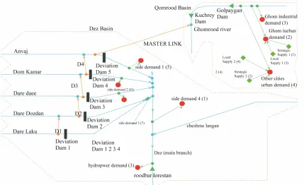
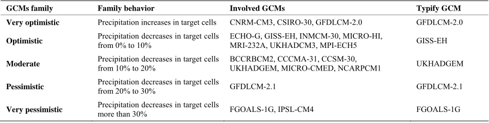
The geographic position of Dez and Ghomrood (Qom- rood) basins in Iran is illustrated in Figure 1. Dez basin is located in the western Zagros massif by high precipita- tion and significant seasonal rainfall; on the other hand, Ghomrood (Qomrood) basin is located in the central arid region. An under construction transmission link will col- lect water from five local branches in higher altitude and will transfer flow to Ghomrood river where two reservoir (Kuchrey and Golpaygan dams) regulate and dispense the flow. A diagram of the system is shown in Figure 2. MAGICC-SCENGEN (Model for Assessment of Green-
[image:2.595.98.500.465.707.2]Figure 2. Schematic scheme and view of allocation model’s interface window of Dez to Qomrood water transmission project, more information are shown in Table 1.
house-gas Induced Climate Change) and its Nineteen GCMs have been used to calculate the change of pre-cipitation in global scale. The resolution of MAGICC- SCENGEN is a mesh of 2.5 × 2.5 degree cells. Figure 1 shows that how forty eight 2.5 × 2.5 degree cells covers Iran and environs, while Dez and Qomrood basins are located in no.19 and no.20 cells. Clearly, the GCMs cannot resolve the spatial structure of climate at the sub- basin scale used in the hydrological model. To down scaling precipitation changes in local scale we used re-verse-distance factors by utilizing results of neighboring cells given from GCMs in global scale. This method is applied by Andersson et al. to down scale precipitation results of GCMs on Okavango River basin [5]. To fore-cast monthly-scale precipitation, we have used GCMs results for monthly variation and compared these with historical monthly distribution to approach a basic monthly distribution function for each GCM-GHE sce- nario. Mitchell et al. have employed this method to fore- cast Europe and the globe climate factors [12]. In order to make more detailed grid network in the basin area, a minor mesh involving 0.5 × 0.5 degree microcells was generated and was utilized for downscaling.
Forecasted precipitation is used to develop runoff characteristics by utilizing a rainfall-runoff model. In this research historical data of rainfall and flow have been applied to develop monthly flow generator via a linier equilibrium. These generators are used to develop runoff for stochastic series of rainfall. Such simplified models,
linier or non linier, are employed in several researches to forecast runoff in similar cases. Gardner employed ex- ponential equilibrium to assess annual runoff in catch- ments with a wide range of climatic conditions [13]. This method also has been applied by a wide range of re-searchers like Graham, Chen, Benestad, and Carter [14- 17]. It’s very clear that many factors like land use, agri- culture and irrigation patterns which have effects on ba- sin’s hydrologic conductivity, are variable in long time. However, in this level of research scope, these uncertain- ties are inevitable and we neglect their impacts.
Table 1. Assumptions and boundary conditions applied in Dez to Ghomrood (Qomrood) water transmission model. Assumptions and boundary conditions
Transmission model components and parts
Total urban demand of Qom city is estimated 150 MCM/year. 120 MCM/year will be supported by transmission link from Dez basin, 20 MCM/year supported by local resources and 16 MCM/year can support by strategic resources.
Urban demand of Qom city
Industrial demand of Qom city is estimated 20 MCM/year Industrial demand of Qom city
Total urban demand of other cities located in transmission link is estimated 52.25 MCM/year. 20 MCM/year will be supported by transmission link from Dez basin, 20 MCM/year supported by local resources and 10.25 MCM/year can support by strategic resources.
Urban demand of other cities located in transmission link
Kuchrey Dam’s capacity is 207 MCM. Also assumed that 50% of this capacity had been full in January of 2000.
Kuchrey Dam
Golpaygan Dam’s efficient capacity assumed 207 MCM. Also assumed that 50% of this capacity had been full in January of 2000.
Golpaygan Dam
According to the forty year statistical registration, annual inflow of local branches in Dez basin, extrapolated 230 CMC/year by average rate of 7.29 CM/second. Annual and Monthly oscilla-tions have been applied in modeling.
Annual inflow of local branches in Dez basin
According to the forty year statistical registration, annual inflow of Anvaj branch in Dez basin just upstream of deviation dam, extrapolated 19.8 MC/year. Annual and Monthly oscillations have been applied in modeling.
Annual inflow of Anvaj river
According to the forty year statistical registration, annual inflow of Domkamar branch in Dez basin just upstream of deviation dam, extrapolated 14.67 CMC/year. Annual and Monthly oscil-lations have been applied in modeling.
Annual inflow of Domkamar river
According to the forty year statistical registration, annual inflow of Dare daee branch in Dez basin just upstream of deviation dam, extrapolated 46.55 CMC/year. Annual and Monthly oscil-lations have been applied in modeling.
Annual inflow of dare daee river
According to the forty year statistical registration, annual inflow of Dare dozdan branch in Dez basin just upstream of deviation dam, extrapolated 129.07 CMC/year. Annual and Monthly os-cillations have been applied in modeling.
Annual inflow of dare dozdan river
According to the forty year statistical registration, annual inflow of Dare laku branch in Dez basin just upstream of deviation dam, extrapolated 98.90 CMC/year. Annual and Monthly oscil-lations have been applied in modeling.
Annual inflow of dare laku river
Maximum transfer capacity of master link is 23 CM/second Transmission capacity of master link between
Dez and Qomrood basins
According to the forty year statistical registration, annual incoming of Cheshme langan branch in Dez basin just upstream of junction by main river of Dez, extrapolated 700 CMC/year by aver-age rate of 22.19 CM/second. Annual and Monthly oscillations have been applied in modeling. Annual incoming of Cheshme langan river
Rudbar Loresatan Dam and power planet designed for capacity of 228 MCM and 450 MegaWatt in normal water years.
Rudbar Loresatan Dam
Side demand between deviation point and junction by Cheshme langan river in Dez basin is estimated to be 60 MCM/year.
Side river demand
A 50-50 allocation for up and downstream PA protocol
Minimum allocation to Downstream = 160 MCM/y FD protocol
Minimum allocation to Upstream = 160 MCM/y FU protocol
About 1.15 billion USD just for transmission links, storage dam and refinery facilities (USD equivalency index of 2006)
Table 2. GCMs families and their definitions in this research.
GCMs family Family behavior Involved GCMs Typify GCM
Very optimistic Precipitation increases in target cells CNRM-CM3, CSIRO-30, GFDLCM-2.0 GFDLCM-2.0
Optimistic Precipitation decreases in target cells from 0% to 10% ECHO-G, GISS-EH, INMCM-30, MICRO-HI, MRI-232A, UKHADCM3, MPI-ECH5 GISS-EH
Moderate Precipitation decreases in target cells from 10% to 20% BCCRBCM2, CCCMA-31, CCSM-30, UKHADGEM, MICRO-CMED, NCARPCM1 UKHADGEM
Pessimistic Precipitation decreases in target cells from 20% to 30% GFDLCM-2.1 GFDLCM-2.1
Very pessimistic Precipitation decreases in target cells more than 30% FGOALS-1G, IPSL-CM4 FGOALS-1G
Table 3. Results of GCMs for precipitation and derived runoff in basin scale. Forecasted change of annual precipitation
(2050)
Calculated change of average runoff in the basin via rainfall-runoff model (2050)
GCMs family Typify GCM
A1 A2 B1 B2 A1 A2 B1 B2 Avg.
Very optimistic GFDLCM-2.0 +8.73 +8.96 +7.10 +7.13 +13.10 +13.44 +10.56 +10.70 +11.97
Optimistic GISS-E –4.04 –3.57 –4.00 –4.75 –6.06 –5.36 –6.00 –7.13 –6.13
Moderate UKHADGEM –15.5 –13.7 –13.2 –14.6 –23.25 –20.67 –19.89 –21.93 –21.43
Pessimistic GFDLCM-2.1 –25.3 –23.8 –21.4 –23.3 –37.95 –35.70 –32.10 –34.95 –35.17
Very pessimistic FGOALS-1G –34.4 –32.4 –30.1 –34.8 –51.60 –48.60 –45.15 –52.60 –49.35
-1999. If this reduction happens in a linier pattern, de- crease rate will be something between 5 to 20 percent for 2050 horizon. It can be a great confirmation for general results given by medium of GCMs. IPCC results are shown in Figure 3 [18,19].
3. Water Allocation Model and Water
Transmission Protocols
In this paper, Water Evaluation and Planning (WEAP) have been used as a tool to model the basins. Mathematic equations were applied for modeling water transmission protocol as controllable valves in master transmission links. Table 1 illustrates initial figures and boundary conditions of the model. The model runs five GCMs outputs, four different climate scenarios and three trans- mission protocols. In this research, we analyzed three common sharing rules which have been described by Ansink & Ruijs [20]. General form of these Protocols and their policies are shown below:
Proportional Allocation (PA): upstream users receives
αQt and downstream users receives (1 − α) Qt, with 0 < α < 1;
Fixed Upstream Allocation (FU): upstream users re- ceives min {β, Qt} and downstream users receives Max {Qt −β, 0}, with 0 < β< E (Qt);
Fixed Downstream Allocation (FD): upstream users receives max {Qt − γ, 0} and downstream users receives Min {γ, Qt}, with 0 <γ < E (Qt).
In this definition, upstream is defined as the basin which can control transferred flow and downstream is the
Figure 3. Large-scale relative changes in annual runoff for the period 2090-2099, relative to 1980-1999 [18]. White ar-eas are where less than 66% of the ensemble of 12 models agreed on the sign of change, and hatched areas are where more than 90% of models agree on the sign of change.
basin which cannot control it. It is clear that water trans- mission projects and its policies are strongly related to socio-economic and politics indicators. This fact obvi- ously can be seen in big and governmental projects, where politic force is the most important factor to stimu- late the project [21]. Thus in such cases, like Dez to Qomrood water transmission project in Iran, due to gov-ernment domination, all controls are under power of cen-tral government, however, in this research we assume principle basin (Dez) as upstream and destination basin (Qomrood) as downstream.
4. Results of Water Allocation Model
dictions; one solution to this problem is to offer a series of weighted predictions developed by various aspect of climate prediction science. In order to gain clear results, final result should be interpreted by logical indexes which contain some sort of sustainability and analogical figures. Three tangible indexes are defined here to evalu- ate the efficiency of three water transmission protocols. The indexes are based on water and energy themes of CSD Indicators of Sustainable Development of UN with considering total population who gain benefits from the project [22]. These indicators are shown in Table 4.
Table 5 shows the final results of PA, FU, and FD transfer protocols for the three sustainability indexes and for A1-AIM scenario. In this table, we have considered the weight of each GCMs family based on climate pre- diction science to get more clear results. In these predic- tions we assume a series of Per-Capita indexes which will be used in next calculations. As it can be inferred from Table 3, a notable result of GHE-GCM models is that in this region the final results strongly depend on GCMs and the effect of climate scenarios is ignorable. Consequently the results are illustrated just for A1-AIM climate scenario and results gained from other climate scenarios are omitted in order to save the reader’s time. A swift glance on the final results shown on Table 5 in- dicates that there are significant differences between the performances of different protocols in each specific sec- tor. All these three allocation protocols (Fix downstream, Fix upstream, and Proportional allocation) cause similar figures for hydroelectric section which may happen ow- ing to the location of the power planet supplied by the other branches from the eastern part of Dez basin. For
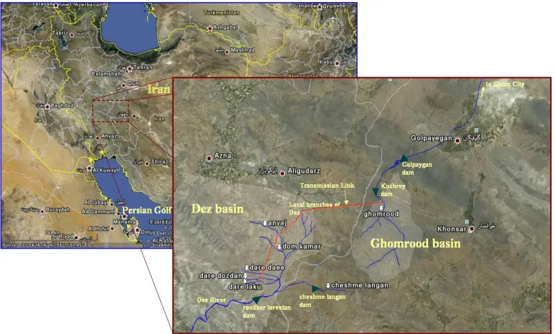
agriculture sector, there is a considerable difference be- tween the result of FU and other protocols, but the most significant variance is observed for the urban demand. More than 2,424,000 of people will be supplied by stan-dard per capita fresh water if FD protocol is selected. The figure shows 2,123,000 for PA protocol and 2,013,000 people for FU. Furthermore, total supplied people by the system exceed more than 2,875,000 for FD protocol, considerably more than 2,576,000 and 2,480,000 for PA and FU respectively. As a common rule, Fix allocation to the main basin (in this case FU) has the minimum dis- rupting effects on a hydrologic system in comparison with the other protocols. In addition, FU protocol con- tains less social conflicts than other protocols because it ensures a minimum flow for the main basin in which stakeholders can’t adapt themselves easily with instance changes caused by the project. The figures illustrated in Table 5 are provided by probability diagrams which are directly produced by water allocation model. As a sample, Probability diagram for the volume of transferred water is shown in Figure 4.
By considering a budget about 1.15 billion US$ for the project, Table 6 illustrates people who will be covered by different aspects of welfare indexes for each 1000 US$ investment in the project. These figures don’t con- tain second round of expenditure like social issues and real cost of environmental damages of construction and operation. But as a swift glance they provide figures for a constructed project which is exist willy-nilly.
5. Conclusion
[image:6.595.58.540.514.738.2]If we just focus on total supported population, FD proto-
Table 4. Comprehensive indexes which have been used in this research, based on “UN: Indicators of sustainable development” definitions [22]. Per-capita indexes are shown in the last column are taken from different resources.
Them Sub-Them Indicator description in UN guideline 2007
Comprehensive indexes which have been used in this research Per-Capita Index Consumption and production patterns Annual energy consumption, total and by main user category
Share of renewable energy sources in total energy use
Access to energy Percentage of population using solid fuels for cooking
Total population who are supplied by
hydro-electricity
2100 Kwh/y (US Energy information administration, 2010)
Sanitation Proportion of population using an improved sanitation facility Poverty
Drinking water Proportion of population using an improved water source
Proportion of total water resources used
Freshwater Water quantity
Water use intensity by economic activity
Total population who are supplied by urban water system
(180 liters/day)
Land Agriculture Arable and permanent cropland area
Total population who are supplied by agricultural production
Table 5. Results of sustainable indicators for FD protocol in face climate change in dez to Qomrood water transmission project, 2000-2050 duration, A1-AIM climate scenario.
Results for 2000-2050 duration (A1-AIM Climate scenario )
Average of hydroelectric
energy production (Gwh/y) Average of annual urban watersupplying (MCM/y)
Average of annual agricultural supplying
involving side rural demand (MCM/y)
Project success (forecasted water transfer/projected
figure)
Water Transmission Protocols Forecast type
Weight of assessment base on 19
PA FU FD PA FU FD PA FU FD PA FU FD
Very optimistic 3 980 980 980 161 159 168 59 59 59 97% 93% 99%
Optimistic 7 880 980 980 160 143 165 57 59 55 96% 84% 98%
Moderate 6 811 852 812 124 126 155 50 56 49 74% 70% 92%
Pessimistic 1 673 703 654 109 99 145 42 53 41 65% 55% 86%
Very pessimistic 2 534 585 515 83 77 130 34 49 31 32% 38% 77%
Weighted average of assessments 864 883 861 138 131 158 52 57 51
[image:7.595.59.535.337.694.2]Supplied population 411,203 420,677 409,925 2,123,077 2,013,765 2,424,291 42,191 46,085 41,121 80.84% 74.63% 93.42%
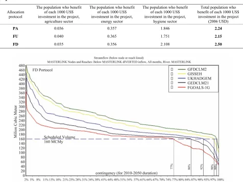
Table 6. The population who make a profit of different aspects of welfare for each 1000 USD investment in the water transfer project.
Allocation protocol
The population who benefit of each 1000 US$ investment in the project,
agriculture sector
The population who benefit of each 1000 US$ investment in the project,
energy sector
The population who benefit of each 1000 US$ investment in the project,
hygiene sector
Total population who benefit of each 1000 US$ investment in the project
(2006 USD)
PA 0.036 0.357 1.846 2.24
FU 0.040 0.365 1.751 2.15
FD 0.035 0.356 2.108 2.50
col will supply a larger group of people. However, PA and FU protocols will put a slighter pressure on the stakeholders who live in the main basin. As a conclusion, there is a tradeoff between the benefit and difficulties of each protocol, but if the economic costs of the project are considered, FD protocol will illustrate its efficiency be- sides more supplied people. FD protocol will achieve more than 93% of the project’s aim in duration from 2010 to 2050 whereas Table 5 shows 80.84% and 74.63% for PA and FU. Current results are rational because FD protocol focuses on maximum possible water transmis- sion in this case; while FU protocol looks for minimum water transmission and PA has a moderate behavior. This research contains the result of the first layer of climate change impacts and a governmental project with consi- dering its special limits. It’s recommended to Future re- searches to focus on the second layer of socio-economic affairs and consider real cost of project as an effective item. In addition, some social issues like immigration to constructed areas and effects of new reservoirs, rate of job cutting, governmental subsides on agriculture and hy- dropower and other factors should be considered. These factors are important to develop an unbiased model which can help water resources managers to have a clear image of the future, and have a multi-criteria knowledge about the real cost and benefits of each protocol.
REFERENCES
[1] G. J. van Oldenborgh, F. J. Doblas-Reyes, B. Wouters and W. Hazeleger, “Skill in the Trend and Internal Vari-ability in a Multi-Model Decadal Prediction Ensemble,”
Climate Dynamics, Vol. 3, No. 7, 2012, pp. 1263-1280. doi:10.1007/s00382-012-1313-4
[2] Y. Chikamoto, M. Kimoto, M. Ishii, T. Mochizuki, T. Sakamoto, H. Tatebe, Y. Komuro, M. Watanabe, T. No- zawa, H. Shiogama, M. Mori, S. Yasunaka and Y. Imada, “An Overview of Decadal Climate Predictability in a Multi-Model Ensemble by Climate Model MIROC,” Cli- mate Dynamic, 2012.
[3] H. Kunstmann, G. Jung, S. Wagner and H. Clotte, “Inte- gration of Atmospheric Sciences and Hydrology for the Development of Decision Support Systems Sustainable Water Management,” Physics and Chemistry of the Earth, Vol. 33, No. 1-2, 2008, pp. 165-174.
doi:10.1016/j.pce.2007.04.010
[4] A. Serrat-Capdevila, J. B. Valdésa, J. G. Péreze, K. Baird, J. Mafa and T. Maddock, “Modeling Climate Change Impacts and Uncertainty on the Hydrology of a Riparian System: The San Pedro Basin (Arizona/Sonora),” Journal of Hydrology, Vol. 347, No. 1-2, 2007, pp. 48-66. doi:10.1016/j.jhydrol.2007.08.028
[5] L. Andersson, J. Wilk, M. C. Todd, D. A. Hughes, A. Earle, D. Kniveton, R. Layberry and H. G. Savenije, “Impact of Climate Change and Development Scenarios on Flow Patterns in the Okavango River,” Journal of
Hy-drology, Vol. 331, No. 1-2, 2006, pp. 43-57. doi:10.1016/j.jhydrol.2006.04.039
[6] A. Wolf, “Conflict and Cooperation along International Waterways,” Water Policy, Vol. 1, No. 2, 1998, pp. 251- 265. doi:10.1016/S1366-7017(98)00019-1
[7] M. Giordano and A. Wolf, “Sharing Waters: Post-Rio International Water Management,” Natural Resources Forum, Vol. 27, No. 2, 2003, pp. 163-171.
doi:10.1111/1477-8947.00051
[8] R. Ghanadan and J. B. Koombey, “Using Energy Scenar-ios to Explore Alternative Energy Pathways in Califor-nia,” Energy Policy, Vol. 33, No. 9, 2005, pp. 1117-1142. doi:10.1016/j.enpol.2003.11.011
[9] A. Oniszk-Poplawska and M. Rogulska, “Renewable- Energy Developments in Poland to 2020,” Applied En-ergy, Vol. 1-3, No. 76, 2003, pp. 101-110.
doi:10.1016/S0306-2619(03)00051-5
[10] M. Eames, “The Development and Use of the UK Envi-ronmental Future Scenarios: Perspectives from Cultural Theory,” Greener Management International, Vol. 37, 2002, pp. 53-70.
[11] K. Ito and Y. Uchiyama, “Study on GHG Control Sce-narios by Life Cycle Analysis—World Energy Outlook until 2100,” Energy Conversion and Management, Vol. 38, 1997, pp. 607-614.
doi:10.1016/S0196-8904(97)00004-6
[12] T. D. Mitchell, T. R. Carter, P. D. Jones, M. Hulme and M. New, “A Comprehensive Set of High-Resolution Grids of Monthly Climate for Europe and the Globe: The Observed Record (1901-2000) and 16 Scenarios (2001- 2100),” Tyndall Centre Working Paper No. 55, 2004. [13] L. R. Gardner, “Assessing the Effect of Climate Change
on Mean Annual Runoff,” Journal of Hydrology, Vol. 379, No. 3-4, 2009, pp. 351-359.
doi:10.1016/j.jhydrol.2009.10.021
[14] L. Graham, J. Andréasson and B. Carlsson, “Assessing Climate Change Impacts on Hydrology from an Ensemble of Regional Climate Models, Model Scales and Linking Methods: A Case Study on the Lule River Basin,” Cli-mate Change,Vol. 81, 2007, pp. 293-307.
doi:10.1007/s10584-006-9215-2
[15] D. L. Chen, et al., “Using Statistical Downscaling to Quantify the GCM-Related Uncertainty in Regional Cli-mate Change Scenarios: A Case Study of Swedish Pre-cipitation,” Advances in Atmospheric Sciences, Vol. 23, 2006, pp. 54-60. doi:10.1007/s00376-006-0006-5
[16] R. E. Benestad, “Tentative Probabilistic Temperature Scenarios for Northern Europe,” Tellus Series A: Dyna- mic Meteorology and Oceanography, Vol. 56, 2004, pp. 89-101.
[17] T. R. Carter, et al., “Developing and Applying Scenarios in Climate Change: Impacts, Adaptation, and Vulnerabil-ity IPCC,” Cambridge UniversVulnerabil-ity Press, Cambridge, 2001, pp.145-190.
[19] B. C. Bates, Z. W. Kundzewicz, S. Wu and J. P. Palutikof, “Climate Change and Water. Technical Paper of the In-tergovernmental Panel on Climate Change, IPCC Secre-tariat,” Geneva, 2008.
[20] E. Ansink and A. Ruijs, “Climate Change and the Stabil- ity of Water Allocation Agreements,” Environmental and Resource Economics, Vol. 41, 2008, pp. 133-287. doi:10.1007/s10640-008-9190-3
[21] B. Gumbo and P. van der Zaag, “Water Losses and the Political Constraints to Demand Management: The Case of the City of Mutare, Zimbabwe,” Physics and Chemis-try of the Earth, Vol. 27, No. 11-22, 2002, pp. 805-813. doi:10.1016/S1474-7065(02)00069-4

![Table 4. Comprehensive indexes which have been used in this research, based on “UN: Indicators of sustainable development” definitions [22]](https://thumb-us.123doks.com/thumbv2/123dok_us/9299887.428530/6.595.58.540.514.738/table-comprehensive-indexes-research-indicators-sustainable-development-definitions.webp)