Patron: Her Majesty The Queen Rothamsted Research Harpenden, Herts, AL5 2JQ
Telephone: +44 (0)1582 763133 Web: http://www.rothamsted.ac.uk/
Rothamsted Research is a Company Limited by Guarantee Registered Office: as above. Registered in England No. 2393175. Registered Charity No. 802038. VAT No. 197 4201 51. Founded in 1843 by John Bennet Lawes.
Rothamsted Repository Download
C1 - Edited contributions to conferences/learned societies
Thompson, R. and Jaffrezic, F. 2003. Modelling and estimation for the
genetic analysis of longitudinal data.
The publisher's version can be accessed at:
• http://isi.cbs.nl/iamamember/CD3/index.html
The output can be accessed at: https://repository.rothamsted.ac.uk/item/8922v.
© 14 August 2003, Please contact [email protected] for copyright queries.
Modelling and Estimation for the Genetic Analysis of
Longitudinal Data
Robin Thompson 1,2 and Florence Jaffrezic 3
1 Rothamsted Research, Harpenden,Herts AL5 2JQ,England, 2Roslin Institute (Edinburgh), Roslin,
Midlothian EH25 9PS,Scotland,3 INRA,SGQA,78352,Jouy-en-Josas,France.
1 INTRODUCTION
In animal breeding situations we are interested in predicting future performance .Over time the number and types of data available have gradually increased .We have expanded from analyses on single traits ,taking into account relationships of animals with their father and ignoring environmental effects into analyses that include several traits ,taking account of all genetic relationships and realistic environmental models .The basic model is a mixed linear model with predictions based on best linear unbiased prediction (BLUP,Henderson,1973).Residual maximum likelihood (REML,Patterson and Thompson ,1971) is often the method of choice for estimation of variance parameters.We discuss algorithms that allow estimation in lage indusrial sized populations.There has recently interest in developing estimation methods for longitudinal data ,for example the so called test day models for milk yield in dairy cattle where information of a series of measurements are combined to give predictions for total lactation yield and other components of the lactation curve.
2 RESIDUAL MAXIMUM LIKELIHOOD ESTIMATION
.
We consider a linear model y=Xb+Zu+e with var(y)= ZGZ‘ +R , var(u)= G and var(e)=R. The residual log-likelihood(REML) is of the form
X) 1 V X logdet( logdet(V) ) bˆ X (y 1 V ) bˆ X (y α
L − ′ − − − − ′ −
This is different from the usual likelihood form in that it is a function of error contrasts – contrasts that do not tell us about fixed effects. This difference has two consequences, the use of the weighted least squares estimate of b, bˆ ,given by X′V−1Xbˆ=X′V−1y
The term in det(X′V−1X)that is sometimes thought of as a penalty function because the fixed effects are not known. Mixed model equations (Henderson, 1973) pay an important part in the analysis process. These are of the form
− ′ − ′ = − + − − − − y 1 R Z y 1 R X uˆ bˆ 1 G Z 1 R Z' X 1 R Z' Z 1 R X' X 1 R X'
Terms derived from these include prediction error variances found from writing the mixed model equations as Cs = R so that
1 C u uˆ bˆ
var = − −
It is often useful to express relevant quantities in terms of the projection matrix 1 V X 1 X) 1 V X X( 1 V
P= − − ′ − − ′ −
X) 1 V X log( logdet(V) Py y α
L ′ − − ′ −
Estimation of a variance parameter θi involves setting to zero the first derivatives
[
P( V/ θi)]
tr )Py i θ V/ P( y i θ
L/∂ = ′ ∂ ∂ − ∂ ∂
These could be thought of equating a function of the data to its expectation. normally finding a maximum of the likelihood requires an iterative scheme. One suggested by Patterson and Thompson (1971) this is based on the expected value of the second differential that is
)P] i θ V/ )P( i θ V/ tr[P( (1/2) ) 2 i θ L/ 2
E(∂ ∂ = − ∂ ∂ ∂ ∂
This is called the Expected Information. Using the first and second differentials we can update
θ using the rate that all the terms from solution of MME and C-1 for example
θ). L/ ( 1 EInf θ θˆ = + − ∂ ∂
Whilst this development is very direct, later developments tried to take account of the structure to reduce the computational effort An alternative algorithm was suggested by Dempster, Laird and Rubin (1987).This EM algorithm is based on thinking of the random effects as `missing’. The estimation is based on using sσˆg2=u′u+PEV(u) writing this as
], ) i θ G/ ( 1 tr[V 2 g sσ y 1 )V i θ G/ ( 1 V y 2 g σˆ
s = ′ − ∂ ∂ − + − − ∂ ∂
We see this as a manipulation of equating the first differential to zero. It can be also written
θ) L/ ( 1 Inf θ
θˆ = + − ∂ ∂ with Inf representing the information on the complete data. One
advantage of this method is σg2 that stays in the parameter space σg2 ≥0.
Another advantage is that there is an increase in likelihood in each iteration. Disadvantages are that the method can be slow to converge (indeed this method is said to be the most widely used in terms of numbers of iterations) and it requires the inversion of C in each iteration.
An important advance was the rediscovery (Misztal and Perez-Enriso, 1993) of an algorithm (Takahashi, et al. 1973) that allowed the calculation of the `relevant’ terms in the inverse of C required for forming the first differentials without calculating all the elements of the inverse. This result allowed the implementation of EM algorithms to estimate variance parameters, (Misztal, 1994) for bigger problems. These were an improvement on derivative free methods but could still be slow to converge. To reduce the computation of the information matrices Thompson and co-workers (Johnson and Thompson, 1995, Gilmour et al., 1995, and Jensen et al., 1997) suggested using an alternative information matrix.
The second differential of C with respect to θi and θj.
)] j θ V/ )P( i θ V/ (1/2)tr[P( )] j θ i θ L/ 2 E[( and Py ) j θ V/ )P( i θ V/ P( y )] j θ V/ )P( i θ V/ (1/2)tr[P( ) j θ i θ L/ 2 ( ∂ ∂ ∂ ∂ − = ∂ ∂ ∂ ∂ ∂ ∂ ∂ ′ − ∂ ∂ ∂ ∂ = ∂ ∂ ∂
Both these terms often called observed and expected information are difficult to calculate but
the average [AI[(∂2L/∂θi∂θj)]=−(1/2)y′P(∂V/∂θi)P(∂V/∂θj)Py can be calculated by
using )Py(∂V/∂θi and (∂V/∂θj)Py as working variables and obtaining the residual
3 LONGITUDINAL DATA
We assume the observed pheotypic tragectory can be decomposed as Y(t)=µ(t) + g(t) + ,e(t) +ε
,where µ(t) is a function of t,g(t) is the genotypic mean function of Y(t), ε is the residual variation ,assumed normally distributed with unknown variance,g(t) and e(t) are Gaussian variables and represent time (t) dependent genetic and enviromental deviations ,independent od one another with covariance functions G(s,t) and E(s,t). Basically three types of models have been suggested for dealing with genetic longitudinal data.
3.1 Random Regression models. Random regression (RR)models are well known in the context of longitudinal data analysis(Diggle et al.,1994).Often convenient parametric curves as linear functions of t are chosen to summerise the genetic and enviromental deviations.By allowing variances and covariances amongst the regression coefficients one can generate variance matrices as a function of t.Alternatively these matrices can be generated as a way of smoothing previously estimated covariance matrices (Kirkpatrick and Heckman,1989,Meyer and Hill,1997)
3.2 Structured antedependence models. In contrast to starting with a linear formulation one might start with a time series like formulation and think that observations at time t might be explained in terms of previous ones..An antedependence structure of order r is defined by the fact that the ith observation (i> r) given the previous r preceding ones is independent of all previous ones (Gabriel,1962).One can easily generalize this to deal with genetic and enviromental components.In structured antedependance (SAD) models the conditional variuance at time t is modelled using a parametric function of t ,for example a polynomial in t (Nunez-Anton and Zimmerman,2000).
3.3 Character Process models. In these models rather than thinking of a linear model to generate the covariance functions we directly decompose the variance function G(s,t) into terms such as
υ(s)υ(t) ρ(s-t).The variance function υ(t) υ(t) can be written as a polynomial in t and ρ(s-t) describes how the correlation changes with s and t. Jaffrezic and Pletcher(2000) suggest using a transition of t,based on a small number of parameters, as a way of introducing non-stationarity. 4 COMPARISONS FOR UNIVARIATE ANALYSIS
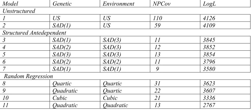
F. Jaffrezic (Ph. D thesis,2001) carried out an extensive investigation of a variety of simulated covariance structures and empirical data and found under most circumstances that structured antedependence and character processes provide the best description of the underlying covariance structure.One example used by Jaffrezic et al.(2002) was based on an analysis of a data set of 9277 cows from 464 bulls with 10 records per animal.Table1 shows that a SAD mdel of first order for the genetic part and third order for the enviromentasl part has a higher order likelihood than a quartic random regression with far fewer parameters (11 instead of 31) 5 DISCUSSION
These analyses show that CP and SAD models offer advantages to random regressions to fit covariance structures that occur in genetic analysis with fewer parameters.We have recently found that such advantages carry over to multivariate analyses(Jaffrezic et al., ,2003) building on work of Sy et al.(1997) with even bigger reductions of parameters from RR models and often very similar models being useful for different traits. One advantage of RR models is that for half-sib data sire and animal models are equivalent.This simplification does not hold for CP models.In one particular case Jaffrezic et al. (2002) the animal model parameterization was better because it allowed a more appropriate model for the enviromental covariance matrix. 6 CONCLUSION
We have discussed estimation methods and models that allow more flexible models of genetic data.
REFERENCES
Diggle, PJ, Liang, KY & Zeger, SL (1994) “Analysis of Longitudinal Data”. Oxford ,Clarendon Press.
Gabriel,K.R.(1962) Ann. Math. Stat. 33:201-212.
Jaffrezic, F. and Pletcher, S.D. (2000) Genetics 156 ,913-922.
Jaffrezic, F,White IMS, Thompson R, Visscher PM (2002) J. Dairy Sci.,85,968-975. Jaffrezic. F, Thompson R. ,Hill, W.G. (2003) Genet. Res. (in press)
Gilmour, A.R., Thompson, R. & Cullis, B.R. (1995) Biometrics 51: 1440-1450.
Gilmour, A.R.,Gogel, B.J.,Cullis, B.R.,Welham, S.J.,Thompson, R. (2002) ASREML User Guide 1.0 .VSN International Ltd. ,Hemel Hempsted HP1 1ES.
Henderson, C.R. (1973) In: Proc. Animal Breeding and Genetics Symposium in Honour of Dr. Jay L. Lush, Champaign, Illinois:10-41.
Henderson,C.R, (1975) Biometrics 31: 3-447.
Hofer, A. (1998) J. Anim. Breed. Genet. 115: 247-265.
Jensen, J , Mantysaari, E , Madsen, P., & Thompson,R. (1997) J. of Indian Soc. Of Agric. Sci. 49: 215-236.
Johnson, D.L. & Thompson, R. (1995) J. Dairy Sci , 78,: 449-456. Kirkpatrick,,m. and Heckman, N.(1989) J. Math. Biol. 27,427-450. Meyer, K. and Hill, W.G.(1997) Livest. Prod. Sci. 149, 185-200. Misztal, I. & Perez-Enciso, M. (1993) J. Dairy Sci. 76: 1479-1483. Misztal, I. (1994) J. Anim. Breed. Genet. 111: 346-355.
Nunez-Anton, V. and Zimmerman, D. I.(2000) Biometrics, 56,699-705. Patterson, H.D. & Thompson, R. (1971). Biometrika, 58:545-554 Smith, S.P. & Graser, H.-U. (1986) J. Dairy Sci. 69: 1156-1165.
Sy ,J.P.,Taylor,J.M.G.,Cumberland,W.G.(1997) Biometrics , 53:542-555.
Takahashi, K., Fagan, J. & Chin, M.S. (1973) In Proc. 8th Inst. PICA Conf.Minneapolis: 63. RÉSUMÉ
Le but de cet exposé est tout d’abord de présenter les différentes procédures d’estimation proposées pour l’estimation REML des composantes de la variance, dont l’algorithme EM et un algorithme de second ordre basé sur la matrice d’Average Information. Nous présenterons ensuite trois types de modèles proposés pour l’analyse des données longitudinales : la aléatoire, les modèles antédépendants structuraux et les modèles à processus. La comparaison de ces différents approches dans une analyse génétique de données de production laitière montre l’intérêt des modèles antédépendants qui permettent une meilleure modélisation de la structure de covariance que les modèles de régression aléatoire, tout en nécessitant beaucoup moins de paramètres.
Table 1 Model comparisons for the genetic analysis of lactation curves for dairy cattle(NPCov: number of parameters in the covariance structure , LogL :Log Likelihood,US Unstructured covariance matrix,SAD(I): structured model of order I)
Model Genetic Environment NPCov LogL
Unstructured
1 US US 110 4126
2 SAD(1) US 59 4109
Structured Antedependent
3 SAD(1) SAD(3) 11 3845
4 SAD(2) SAD(3) 12 3852
5 SAD(3) SAD(3) 13 3854
6 SAD(2) SAD(2) 11 3796
7 SAD(1) SAD(1) 9 3580
Random Regression
8 Quartic Quartic 31 3623
9 Quadratic Quartic 22 3607
10 Cubic Cubic 21 3336