Solution of Stochastic Quadratic Programming with Imperfect Probability Distribution Using Nelder Mead Simplex Method

(1)

ISSN Online: 2327-4379 ISSN Print: 2327-4352

DOI: 10.4236/jamp.2018.65095 May 31, 2018 1111 Journal of Applied Mathematics and Physics

Solution of Stochastic Quadratic Programming

with Imperfect Probability Distribution Using

Nelder-Mead Simplex Method

Xinshun Ma

*

_{, Xin Liu}

Department of Mathematics and Physics, North China Electric Power University, Baoding, China

Abstract

Stochastic quadratic programming with recourse is one of the most important topics in the field of optimization. It is usually assumed that the probability distribution of random variables has complete information, but only part of the information can be obtained in practical situation. In this paper, we pro-pose a stochastic quadratic programming with imperfect probability distribu-tion based on the linear partial informadistribu-tion (LPI) theory. A direct optimizing algorithm based on Nelder-Mead simplex method is proposed for solving the problem. Finally, a numerical example is given to demonstrate the efficiency of the algorithm.

Keywords

Stochastic Quadratic Programming, LPI, Nelder-Mead

1. Introduction

Stochastic programming is an important method to solve decision problems in random environment. It was proposed by Dantzig, an American economist in 1956 [1]. Currently, the main method to solve the stochastic programming is to transform the stochastic programming into its own deterministic equivalence class and using the existing deterministic planning method to solve it. According to different research problems, stochastic programming mainly consists of three problems: distribution problem, expected value problem, and probabilistic con-straint programming problem. Classic stochastic programming with recourse is a type of expected value problem, modeling based on a two-stage deci-sion-making method. It is a method by making decisions before and after

ob-How to cite this paper: Ma, X.S. and Liu, X. (2018) Solution of Stochastic Quadratic Programming with Imperfect Probability Distribution Using Nelder-Mead Simplex Method. Journal of Applied Mathematics and Physics, 6, 1111-1119.

https://doi.org/10.4236/jamp.2018.65095 Received: April 16, 2018

Accepted: May 28, 2018 Published: May 31, 2018 Copyright © 2018 by authors and Scientific Research Publishing Inc. This work is licensed under the Creative Commons Attribution International License (CC BY 4.0).

http://creativecommons.org/licenses/by/4.0/

(2)

DOI: 10.4236/jamp.2018.65095 1112 Journal of Applied Mathematics and Physics serving the value of a variable. With regard to the theory and methods of two-stage stochastic programming, a very systematic study has been conducted and many important solutions have been proposed [2]. In these methods, the dual decomposition L-shape algorithm established in the literature [3] is the most effective algorithm for solving two-stage stochastic programming. It is based on the duality theory, and the algorithm converges to the optimal solution by determining the feasible cutting plane and optimal cutting, and solving the main problem step by step. This method is essentially an external approximation algorithm that can effectively solve the large-scale problems that occur after the stochastic programming is transformed into deterministic mathematical pro-gramming. Abaffy and Allevi present a modified version of the L-shaped method in [4], used to solve two-stage stochastic linear programs with fixed recourse. This method can apply class attributes and special structures to a polyhedron process to solve a certain type of large-scale problems, which greatly reduces the number of arithmetic operations.

While the stochastic programming is transformed into the corresponding equivalence classes, it is generally a nonlinear equation. In recent years, with the introduction of new theories and methods for solving nonlinear equations, espe-cially the infinite dimensional variational inequality theories and the application of smoothness techniques that have received widespread attention in recent years [5][6][7], a stochastic programming solution method based on nonlinear equation theory is proposed. Chen X. expressed the two-stage stochastic pro-gramming as a deterministic equivalence problem in the literature [8], and transformed it into a nonlinear equation problem by introduced Lagrange mul-tiplier. By using the B-differentiable properties of nonlinear functions, a Newton method for solving stochastic programming is proposed. Under certain condi-tions, the global convergence and local super-linear convergence of the algo-rithm are proved.

(3)

DOI: 10.4236/jamp.2018.65095 1113 Journal of Applied Mathematics and Physics

2. The Model of Stochastic Quadratic Programming with

Imperfect Probability Distribution

Let

(

Ω Σ, ,P

)

be a probability space, _{h h}₌

( )

_ω

_∈_Rm_{is a stochastic vector in} this space, _{C R}_∈ n n× _{be symmetric positive semi-definite and}_{H R}_∈ m m× _be symmetric positive definite. We consider following problem:

( )

T T

, 1 min

2 s.t.

n m

x R y R x Cx c x f y

Ax b Tx y

∈ ∈ + +

≤ =

(1)

where

( )

max_P P

(

,

)

f y _π E g yω

∈

= ₍₂₎

(

_,

)

_max 1 T T

(

( )

)

2 s.t.

m

i _{z R} i

g y z Hz z h y

Wz q

ω ω

∈

= − + −

≤ (3) Here _{x R y R}_∈ n, _∈ m_{are decision variables,}

_{c R A R}

_∈

n

_,

_∈

r n×

_,

_b

_∈

_R

r

_,

_{T R}

_∈

m n× _,

1, 1

m m m

q R W R_∈ _∈ × _{are fixed matrices,} ω∈Rm2 is a random vector with support 2

m

R

Ω ⊆ _,





T

1, , ,2 N

P p p  p is the probability distributions of limited sample set Ω =

(

ω

1, ,

ω

N

)

, that is pi =prob

(

{

ω ω

= i

}

)

. Assumed that the probability distribution of random variable has the following linear partial information:

1

| , N 1; 0, 1, ,

N

i i

i

P R BP d p p i N

π

=

 

= ∈ ≤ = ≥ = 



∑

 

Here _{d R B R}_∈ s, _∈ s N× _{are fixed matrices, assumed the set of probability}

dis-tributions π_{is a polyhedron. Thus the two-stage function can be written as}

( )

(

)

(

)

1

max_P P , max_P N i , i

i

f y _π E g yω _π p g yω

∈ ∈

=

= =

∑

₍₄₎

We call Equations (1)-(3) stochastic quadratic programming with recourse models under LPI.

Chen established a similar stochastic quadratic programming model in [8], but assumed that the probability distribution is completely known, that is the “Max” symbol in Equation (2) does not appear. The above model is a new sto-chastic quadratic programming model based on LPI theory to solve the stochas-tic programming problem with incomplete information probability distribution. Since g y

(

,ωi

)

is the convex function about y ([8]), f y

( )

is also the convex

function about y (see [13]), and then the problems (1)-(3) essentially belong to the convex programming problem. Obviously the recourse function is not diffe-rential, so the Newton method proposed in [8] is no longer applicable. In order to solve this problem, we design a solution based on the improved Nelder-Mead method. The experimental results show that the method is effective.

3. Modified Nelder-Mead

(4)

algo-DOI: 10.4236/jamp.2018.65095 1114 Journal of Applied Mathematics and Physics rithm developed for solving the nonlinear programming, NM algorithm belongs to the modified polyhedron method in nature. It searches for the new solution by reflecting the extreme point with the worst function value through the cen-troid of the remaining extreme points. Experimental shows, compared to ran-dom search, the algorithm can find the optimal solution more efficiently. The NM algorithm does not require any gradient information of the function during the entire optimization procedures, it can handle problems for which the gra-dient does not exist everywhere. NM allows the simplex to rescale or change its shape based on the local behavior of the response function. When the new-ly-generated point has good quality, an extension step will be taken in the hope that a better solution can be found. On the other hand, when the new-ly-generated solution is of poor quality, a contraction step will be taken, re-stricting the search on a smaller region. Since NM determines its search direc-tion only by comparing the funcdirec-tion values, it is insensitive to small inaccuracies in function values.

The classic NM method has several disadvantages in the search process. First, the convergence speed of the algorithm depends too much on the choice of ini-tial polyhedron. Indeed, a too small iniini-tial simplex can lead to a local search, consequently the NM may convergent to a local solution. Second, NM might perform the shrink step frequently and in turn reduce the size of simplex to the greatest extent. Consequently, the algorithm can converge prematurely at a non-optimal solution.

Chang [15] propose a new variant of Nelder-Mead, called Stochastic Neld-er-Mead simplex method (SNM). This method seeks the optimal solution by gradually increasing the sample size during the iterative process of the algo-rithm, which not only can effectively save the calculation time, but also can in-crease the adaptability of the algorithm to prevent premature convergence of the algorithm. This article refers to the design idea of [15] and adds an adaptive random search process to solve problems (1)-(3) in the NM algorithm. The spe-cific process of the algorithm is described as follows:

Firstly, by attaching a Lagrange multiplier vector λ_{, convex problems (1)-(3)} can be written as an unconstrained problem:

( )

_min1 T T

( )

T

(

)

2x Px c x f y Ax b

θ µ = + + +λ − ₍₅₎

(

_,

)

T

x

µ= λ _{, let}

_{µ µ}

1_{, , ,}2 _

_µ

n+1_{be the} _n_₁_{points of n-dimensional space of} n

R , which are not on the same plane. Let

_{µ µ µ}

h, ,s l_{represent the points that} have the highest, second highest, and lowest estimates of function values,

_µ

c_is the centroid of all vertices other than _h_, c 1 i_.

i h

n

µ µ

≠

=

∑

Reflection: since

_µ

h_{is the vertex with the higher value among the vertices,} we can expect to find a lower value at the reflection of

_µ

h_{in the opposite face} formed by all vertices

_µ

i_except

_µ

h_{. Generate a new point}

_µ

r_{, by reflecting}

h

µ

through

_µ

c_{according to}

(

)

with

(

0

)

r c c h

(5)

DOI: 10.4236/jamp.2018.65095 1115 Journal of Applied Mathematics and Physics If the reflected point is better than the second worst, but not better than the best, i.e. _{θ µ}

( ) ( ) ( )

l _<_{θ µ}r _<_{θ µ}s _{, then obtain a new simplex by replacing the}

worst point

_µ

h_{with the reflected point}

_µ

r_.

Expansion: if the reflected point is the best point so far, we can expect to find interesting values along the direction from

_µ

c _to

_µ

r_{, that is if}

( ) ( )

r l

θ µ <θ µ _{, then search direction is favorable, compute the expansion point} using

(

)

with

(

1

)

e c c h

µ =µ +β µ −µ β > _.

If the expanded point is better than the reflected point, that is

( ) ( )

e r

θ µ

<

θ µ

_{, then replace}

_µ

h _by

_µ

e_{, otherwise, obtain a new simplex by} replacing the worst point

_µ

h _{with the reflected point}

_µ

r_.

Contraction: here it is certain that

_{θ µ}

( ) ( )

r _>

_{θ µ}

s _{, in this case, we can} ex-pect that a better value will be inside the simplex formed by all the vertices, then the simplex contracts.

1) If

θ µ

( ) ( ) ( )

s <

θ µ

r <

θ µ

h _{, the contracted point is determined by}

(

)

p c r c

µ

=

µ

+

γ µ

−

µ

_with 0≤ <γ 1, if

_{θ µ}

( ) ( )

p _<

_{θ µ}

h _{, the contraction is} ac-cepted, Replaced

_µ

h_by

_µ

p_.

2) If _{θ µ}

( ) ( )

r _≥_{θ µ}h _{, the contracted point is determined by}

(

)

p c h c

µ

=

µ

+

γ µ

−

µ

_{, if}

_{θ µ}

( ) ( )

p _<

_{θ µ}

h _{, the contraction is accepted. Replaced} h

µ

_by

_µ

p_.

Shrink: although a failed contraction is much rarer, it may happen in some case, In that case, generally we contract towards the lowest point in the expecta-tion of finding a simpler landscape. Replace all points except the best point

_µ

l with

_µ

i₌

_{µ δ µ µ}

l ₊

(

i ₋ l

)

_{. This article uses the following process: when} con-traction fails, using a random search process to generate new points based on fitness of function. Let fitness function be _F

( )

_µi _{= −}_{θ µ}

( )

i ₊_M _{, where}_M_{is a} fully large number, calculate the probability of obtaining

_µ

i _by

( )

1

( )

1

n

i i

i

F µ + F µ

=

∑

. According to the roulette algorithm, get a new point by randomly searched in the neighborhood of the point corresponding to the probability interval. The neighborhood

δ µ

( )

i _of

_µ

i _{is defined as}

( )

i

{

: i min

{

i j , _{j i}

}

δ µ = µ µ µ− ≤ µ −µ ∀ ≠

Algorithm termination condition: There are different criteria to determine the termination conditions of the NM algorithm in practice, in this paper, we use

( ) ( )

( )

,

h l

l

θ µ θ µ

ε θ µ

−

≤

as our convergence criterion.

Parameters choice: The polyhedron transform in the NM algorithm mainly includes four parameters, α _{for reflection,} β _{for expansion and}γ for con-traction, assumed they satisfy the following constraints:

0, 1, ,0 1.

(6)

DOI: 10.4236/jamp.2018.65095 1116 Journal of Applied Mathematics and Physics Algorithm

Choose α >0,β >1,β α> ,0< <γ 1_{, Convergence criterion} ε>0.

Step 1 calculate the function values of n+1 points, rank all points and identify , ,

h s l

k k k

µ µ µ

_{, find} c k

µ

, the centroid of all vertices other than h k

µ

, generating a new point r

k

µ

_{by reflecting point} h k

µ

_through c k

µ

_{according to reflection rule}

(

)

r c c h

k k k k

µ

=

µ

+

α µ

−

µ

_;

Step 2 if

( ) ( )

r l

k k

θ µ

<

θ µ

_{, then the reflection point is expanded using the}

ex-pansion rule

µ

ke=

µ

kc+

β µ

(

kc−

µ

kh

)

, if

θ µ

( ) ( )

ke <

θ µ

kr , then replace

µ

kh by e

k

µ

, otherwise, let r k

µ

replaced h k

µ

, return to Step 4; Step 3 if

( ) ( ) ( )

l r s

k k k

θ µ

<

θ µ

<

θ µ

_{, then let} r k

µ

replaced h k

µ

, go to Step 4, otherwise return to Step 5;

Step 4 if the convergence criterion is met, stop the iteration, otherwise, return to Step 1;

Step 5 if

( ) ( )

r s

k k

θ µ

≥

θ µ

_{, then the simplex contracts.}

(i) if

( ) ( ) ( )

s r h

k k k

θ µ

<

θ µ

<

θ µ

_{, the contraction point is determined by}

calcu-late p c

(

r c

)

k k k k

µ

=

µ

+

γ µ

−

µ

_,

(ii) if

( ) ( )

r h

k k

θ µ

≥

θ µ

_{, the contraction point is determined by calculate}

(

)

p c h c

k k k k

µ

=

µ

+

γ µ

−

µ

_.

In these case, if

( ) ( )

p r

k k

θ µ

<

θ µ

_{, the contraction accepted, If contraction is}

accepted, let p k

µ

replaced h k

µ

, return to Step 4;

Step 6 when all previous Step s fail, we use adaptive random search to gener-ate new points, then return to Step 1.

4. Numerical Experiment

Consider the problem (1)-(3) in which _{X R H I R T}_∈ 3_, _{= ∈} 3 3× _, _{= −}_H_{, and}

2 0 0 1 2 3 6

0 1 0 , 0 1 1 , 3

0 0 1 1 0 1 4

C W q

−             =_ _ =_ − _ =_{ }             4

3 2 1 12

3 , ,

1 2 1 8

2

c A b

−         = −_ _ =_ _ =_{ }     ₋   

Assumed stochastic vector

(

1_{, ,}2 3

)

T

i i i i

ω = ω ω ω

(

i=1,2, ,_ N

)

_is

three-dimensional vector, 1_, 2

i i

ω ω

and 3

i

ω

are independent of each other. We use MATLAB to randomly generate one hundred values for each other. Let

( )

i i

h

ω

=

ω

, we experiment with the effectiveness of the algorithm under the fol-lowing conditions.

Case 1: let N=10, the parameter in the linear part information of the proba-bility distribution π is set to

(

)

(

)

(

)

T

8 8 8 1 8

T

1, ,1 , ,O , ,

1 6,1 8,1 5,1 4,1 7,1 6,1 7,2 7

D B E D

d

×

= =

= 

(7)

DOI: 10.4236/jamp.2018.65095 1117 Journal of Applied Mathematics and Physics

1 10 1 6, 2 10 1 8, , 1 2 10 1

p +p ≤ p + p ≤ _ p +p +_+ p =

The parameters of modified NM method are given, reflection factor α =1, expansion factor β =2_{, contraction factor} γ =0.5_{, convergence criterion}

8

1 10

ε_{= ×} − _.

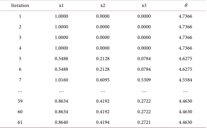
Use MATLAB R2008a to achieve the above problems, Table 1 gives the deci-sion variable x and the function value θ , the calculation result retains four de-cimal places.

The actual running results show that the algorithm terminates after 61 times, the optimal solution is x=

(

0.8634,0.4194,0.2721

)

T, the optimal function value

is

θ

=4.4630. The running time is 28.515197 seconds.

Case 2: To verify the effectiveness of the algorithm, we expand the value of N, let N =100, the parameter in the linear part information of the probability dis-tribution π _{as follows,} D₈=

(

1, ,1_

)

T, B=

(

E8,O , 8 91× D8

)

,

(

_{1 6,1 8,1 5,1 4,1 7,1 6,1 7,2 7}

)

T

d = , that is keep the row of B unchanged, extend the number of random variables to 100, this means

1 100 1 6, 2 100 1 8, , 1 2 100 1

p + p ≤ p +p ≤ _ p +p +_+ p = _{, use MATLAB R2008a} to achieve the above problems again, the result is Table 2.

From Table 2, we can see the program stops at 89 times, the optimal solution is x=

(

0.8659,0.3530,0.2682

)

T_{, optimal function value is}

θ

=4.8989_{. The} running time is 382.307942 seconds. Comparing the results, we find that when the value of N is increased by 10 times, the running time increased by 13 times, this is normal, it need more times to calculate the recourse function. However, the number of iterations of the algorithm is only increased by 1/4, which shows that the algorithm in this paper is effective for solving stochastic programming problems.

[image:7.595.208.540.512.717.2]

Case 3: In order to investigate the sensitivity of the linear partial information constraint condition of the probability distribution to the algorithm, we increase

Table 1. Iterative results.

Iteration x1 x2 x3 θ 1 1.0000 0.0000 0.0000 4.7366 2 1.0000 0.0000 0.0000 4.7366 3 1.0000 0.0000 0.0000 4.7366 4 1.0000 0.0000 0.0000 4.7366 5 0.5488 0.2128 0.0784 4.6275 6 0.5488 0.2128 0.0784 4.6275 7 1.0160 0.6095 0.5309 4.5584

… … … … …

(8)

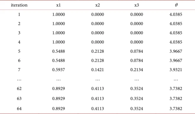
DOI: 10.4236/jamp.2018.65095 1118 Journal of Applied Mathematics and Physics the constraints to observe the change of the optimal solution. Take N=10, and add the following two constraints to the probability distribution, p2+p3≤1 9,

4 5 1 10

p +p ≤ _{, following is the running result,}

From Table 3 we can see, the program stops at 64 times, the optimal solution is x=

(

0.8929,0.4113,0.3524

)

T_{, optimal function value is}θ=3.7382_{, the}

run-ning time is 29.490318 seconds. this shows, on the one hand, as the information of the probability distribution changes from incomplete to complete informa-tion, the objective function values of the models (1)-(3) constructed tend to have better results. On the other hand, there is no significant increase in the number of iterations of the algorithm during the optimization process.

5. Conclusion

[image:8.595.208.539.302.492.2]

For the case that the probability distribution has incomplete information, this

iteration x1 x2 x3 θ 1 1.0000 0.0000 0.0000 5.1179 2 1.0000 0.0000 0.0000 5.1179 3 1.0000 0.0000 0.0000 5.1179 4 1.0000 0.0000 0.0000 5.1179 5 0.5488 0.2128 0.0784 5.0412 6 1.0037 0.6341 0.4862 5.0223 7 1.0037 0.6341 0.4862 5.0223

… … … … …

87 0.8659 0.3530 0.2681 4.8989 88 0.8659 0.3530 0.2681 4.8989 89 0.8659 0.3530 0.2682 4.8989

iteration x1 x2 x3 θ 1 1.0000 0.0000 0.0000 4.0385 2 1.0000 0.0000 0.0000 4.0385 3 1.0000 0.0000 0.0000 4.0385 4 1.0000 0.0000 0.0000 4.0385 5 0.5488 0.2128 0.0784 3.9667 6 0.5488 0.2128 0.0784 3.9667 7 0.5937 0.1421 0.2134 3.9321

… … … … …

[image:8.595.208.538.524.717.2]

(9)

DOI: 10.4236/jamp.2018.65095 1119 Journal of Applied Mathematics and Physics paper establishes a stochastic quadratic programming model with incomplete probability distribution based on LPI theory, and designs an improved Neld-er-Mead algorithm. The numerical examples are used to calculate the results. The results show that the established models and algorithms are reasonable and effective.

References

[1] Dantzig, G.B. and Ferguson, A.R. (1956) The Allocation of Air Craft Routes-An Example of Linear Programming under Uncertainty. Management Science, 3, 23-34.

[2] Birge, J.R. and Louveanx, F. (2003) Introduction to Stochastic Programming. Springer-Verlag, New York.

[3] Slyke, R. and Wets, R. (1969) L-Shaped Linear Programs with Applications to Op-timal Control and Stochastic Programming. SIAM Journal on Applied Mathemat-ics, 17, 638-663. https://doi.org/10.1137/0117061

[4] Abaffy, J. and Allevi, E. (2004) A Modified L-shaped Method. Journal of Optimiza-tion Theory and ApplicaOptimiza-tions, 11, 255-270.

https://doi.org/10.1007/s10957-004-5148-y

[5] Facchinei, F. and Pang, J.S. (2003) Finite-Dimensional Variational Inequalities and Complementarity Problems. Springer-Verlag, New York.

[6] Qi, L. (1993) Convergence Analysis of Some Algorithms for Solving Non-Smooth Equations. Mathematics and Operations Research, 18, 227-244.

https://doi.org/10.1287/moor.18.1.227

[7] Qi, L. and Sun, J. (1993) A Non-Smooth Version of Newton’s Method. Mathemati-cal Programming, 58, 353-367. https://doi.org/10.1007/BF01581275

[8] Chen, X., Qi, L, and Womersley, R.S. (1995) Newton’s Method for Quadratic Sto-chastic Programs with Recourse. Journal of Computational and Applied Mathemat-ics, 60, 29-46. https://doi.org/10.1016/0377-0427(94)00082-C

[9] Abdelaziz, F.B. and Masri, H. (2005) Stochastic Programming with Fuzzy Linear Partial Information on Probability Distribution. European Journal of Operational Research, 162, 619-629. https://doi.org/10.1016/j.ejor.2003.10.049

[10] Abdelaziz, F.B. and Masri, H. (2009) Multistage Stochastic Programming with Fuzzy Probability Distribution. Fuzzy Sets and Systems, 160, 3239-3249.

https://doi.org/10.1016/j.fss.2008.10.010

[11] Zhang, Y. and Ma, X. (2016) A Class Recourse Stochastic Programs Algorithm with MaxEM in Evaluation. Operations Research Transactions, 20, 52-60.

[12] Kofler, E. (2001) Linear Partial Information with Applications. Fuzzy Sets and Sys-tems, 118, 167-177. https://doi.org/10.1016/S0165-0114(99)00088-3

[13] Boyd, S. and Vandenberghe, L. (2004) Convex Optimization. Cambridge University Press, Cambridge. https://doi.org/10.1017/CBO9780511804441

[14] Nelder, J.A. and Mead, R. (1965) A Simplex Method for Function Minimization. The Computer Journal, 7, 308-313. https://doi.org/10.1093/comjnl/7.4.308