One dimensional scaling limits in a planar Laplacian random growth model

arXiv:1804.08462v1 [math.PR] 23 Apr 2018

One-dimensional scaling limits in a planar Laplacian random

growth model

Alan Sola∗1, Amanda Turner †2, and Fredrik Viklund ‡3

1_{Department of Mathematics, Stockholm University, 106 91 Stockholm, Sweden.} 2_{Department of Mathematics and Statistics, Lancaster University, Lancaster LA14YF, UK.}

3_{Department of Mathematics, Royal Institute of Technology, 100 44 Stockholm, Sweden.}

April 24, 2018

Abstract

We consider a family of growth models defined using conformal maps in which the local growth rate is determined by|Φ′

n|

−η_{, where Φ}

nis the aggregate map fornparticles. We establish a scaling limit result in which strong feedback in the growth rule leads to one-dimensional limits in the form of straight slits. More precisely, we exhibit a phase transition in the ancestral structure of the growing clusters: for η > 1, aggregating particles attach to their immediate predecessors with high probability, while forη <1 almost surely this does not happen.

Contents

1 Introduction 2

1.1 Conformal aggregation processes . . . 2 1.2 ALE: Aggregate Loewner Evolution . . . 4

2 Overview of results 5

2.1 A related Markovian model . . . 7 2.2 Overview of the proof of Theorem 1 and organization of the paper . . . 10

3 Loewner flows 12

3.1 Loewner’s equation . . . 12 3.2 Reverse-time Loewner flow . . . 14 3.3 Convergence of Loewner chains . . . 15

4 Analysis of the slit map 16

4.1 The half-plane . . . 17 4.2 The exterior disk . . . 18 4.3 Moment computations . . . 21

∗_{[email protected]}

5 Estimates on conformal maps via Loewner’s equation 23

5.1 Near the tip . . . 24 5.2 Away from the slits . . . 29

6 Ancestral lines and convergence for ALE 36

6.1 Combined derivative estimates . . . 37 6.2 The ancestral lines and convergence theorem . . . 37 6.3 Modifications of the model . . . 41

1

Introduction

1.1 Conformal aggregation processes

Laplacian growth models describe processes where the local growth rate of a piece of the boundary of a growing compact cluster is determined by the Green’s function of the exterior of the cluster. Such growth processes can be used to model a range of physical phenomena, including ones involving aggregates of diffusing particles. Discrete versions can be formulated on a lattice in all dimensions: some famous examples of this type of growth process include diffusion-limited aggregation (DLA) [30], the Eden model [4], or the more general dielectric breakdown model (DBM) [24]. Despite considerable numerical evidence suggesting that the clusters that arise in these processes exhibit fractal features, very few rigorous results are known (for DLA, see [16]) and it remains a formidable challenge to rigorously analyze long-term behavior such as sharp growth rates of the clusters.

One objection that can be leveled at lattice-based models is that the underlying discrete spacial structure could potentially introduce anisotropies in the growing clusters that are not present in the physical setting of the plane or three-space. Indeed, large-scale simulations in two dimensions demonstrate anisotropy along the coordinate axes [5]. This fact provides one motivation for the study of off-lattice versions of aggregation processes. In the plane, such off-lattice models can be formulated in terms of iterated conformal mappings, providing access to complex analytic machin-ery. Clusters produced by these conformal growth processes are initially isotropic by construction, but simulations suggest that in many instances, anisotropic structures appear on timescales where the number of aggregated particles become large compared to the size of the individual constituent particles. Nevertheless, proving the existence of such small-particle limits, whether anisotropic or not, has proved elusive, similarly to the case of lattice-based models.

A fascinating feature of Laplacian growth models is competition between concentration and dispersion of particle arrivals on the cluster boundary. Protruding structures (“branches”) and their endpoints (“tips”) tend to attract relatively many arrivals, but they compete with each other as well as the remainder of the boundary. (Kesten’s discrete Beurling estimate gives an upper bound on the tip concentration in the case of DLA.) The degree to which tips are favored is determined by the exact choice of growth rule, and several models contain one or more parameters that affect concentration, dispersion, and competition [24, 8, 2, 18].

in the sense that growth, which is initially spread out, favors tips very strongly, and eventually collapses onto a single growing slit.

To state our results, we first describe the general class of processes our object of study fits into. Letc>0, and letfc denote the unique conformal map

fc: ∆ ={z∈C:|z|>1} ∪ {∞} →D1 = ∆\(1,1 +d]

having fc(z) = e c

z+_O(1) at infinity, and sending the exterior disk ∆ to the complement of the closed unit disk with a slit of length d = d(c) attached to the unit circle T at the point 1. The capacity increment cand the length dof the slit satisfy

ec

= 1 + d

2

4(1 +d); (1)

in particular, d _≍c1/2 as c _→ 0. In terms of aggregation, the closed unit disk can be viewed as a seed, while the slit represents an attached particle. Typically, we think of the particle as being small compared to the seed.

A general two-parameter framework to model random or deterministic aggregation, based on conformal maps, is given by the following construction. Pick a sequence_{θk}∞k=1 in [−π, π), and let {dk}∞k=1, or, equivalently,{ck}∞k=1, be a sequence of non-negative numbers connected via (1). From

the two numerical sequences _{θk} and {ck}, we obtain a sequence{fk}∞_k=1 of rotated and rescaled

conformal maps, referred to as building blocks, via

fk(z) =eiθkfck(e−

iθk_z).

Finally, we set

Φn(z) =f1◦ · · · ◦fn(z), n= 1,2, . . . . (2)

Each Φn is itself a conformal map sending the exterior disk onto the complement of a compact set Kn⊂C, that is,

Φn: ∆→C\Kn.

The sets _{Kn}∞n=1 are called clusters. They satisfy Kn−1 ⊂ Kn, and model a growing

two-dimensional aggregate formed ofn particles. At infinity, we have

Φn(z) =eCnz+O(1),

where

cap(Kn) =eCn =e Pn

k=1ck ₍₃₎

is the total capacity of thenth cluster.

When modeling random aggregates formed via diffusion, one chooses the angles _{θk}to be iid,

and uniform in [₋π, π). Due to the conformal invariance of harmonic measure, this has the effect of attaching thenth particle at a point chosen according to harmonic measure (seen from infinity) on the boundary of Kn−1. This type of setup has been considered in a number of papers, see

1.2 ALE: Aggregate Loewner Evolution

The main object of study in the present paper is a model we refer to as aggregate Loewner evolution, abbreviated ALE(α, η), with parameters α_∈R and η_∈R. In ALE(α, η), conformal maps Φn are

defined as in (2) as follows.

Initialize by setting Φ0(z) =z and letting F0 be the trivial σ-algebra.

• Fork= 1,2,3, . . ., we letθkhave distribution conditional onFk−1 =F(θ1, . . . θk−1;c1, . . . , ck−1)

given by

hk(θ) = |

Φ′_k−1(eσ+iθ

)_|−ηdθ

R

T|Φ′k−1(e

σ+iθ

)_|−η_dθ. (4)

Here,σ>0 is a regularization parameter, which ensures that the angle distributions are well

defined even though Φ′

k−1(eiθ) has zeros and singularities on T. The parameterσ is allowed

to depend on the basic capacity parameterc. Typically, we shall take

σ =σ(c) =cγ

for some appropriateγ >0.

• Next, we define a sequence of capacity increments fork= 1,2,3, . . . by taking

ck =c|Φ′k−1(e

σ+iθ_k

)_|−α. (5)

We note that ALE(α,0) is the same model as the Hastings-Levitov HL(α) model studied in [8, 3, 28, 14], and in particular ALE(0,0) coincides with the HL(0) model studied in depth in [25, 29]. The Hastings-Levitov model was introduced as a conformal mapping model of dielectric breakdown (DBM) [24], a discrete model in which vertices are added to a growing cluster by drawing bonds from among the neighboring lattice points. At stagen of DBM(η), a point is added to the cluster

Kn by including a neighbor of (j, k)∈Kn with probability

pn (j, k) _→(j′, k′)

= φn(j′, k′)

η

P

(l,m)φn(l, m)η .

Here, summation is over lattice neighbors of Kn and the function φn is discrete harmonic, that is

∆φn= 0 on Z2\Kn, and hasφn= 0 onKn and φn= 1 on some large external circle.

Off-lattice versions of DBM involving non-uniform angle choices determined by the derivative of a conformal map have been considered by several authors. Hastings [6], and subsequently Mathiesen and Jensen [21], study a model that essentially corresponds to ALE(2, η) modulo a slightly different parametrization inη. (In fact, an alternative name for the growth model in this paper could have been DBM(α, η) or HL(α, η), but we have opted for a different terminology to avoid confusion with lattice models, and also to emphasize connections with the Loewner equation, see below.) Hastings argues that large enough exponents, more precisely, forη >3 in our parametrization, the corresponding clusters become one-dimensional; he also points out that the behavior of the models depends strongly on the choice of regularization.

distribution which depends on the power of the derivative of the cluster map, as in (4), but with an additional term involving the Gaussian Free Field due to the presence of Liouville quantum gravity. In the construction of QLE, capacity increments are kept constant, as for ALE(0, η). However, each particle in QLE is constructed as an SLE curve, rather than the straight slits used in ALE.

Common to all conformal mapping models of Laplacian growth is the difficulty that derivatives of conformal mappings do not remain bounded away from 0 or _∞ as they approach the boundary and therefore the mapθ_{7→ |}Φ′

n(eiθ)|−1 can be very badly behaved. For instance, even whenn= 1,

|Φ′

n(eiθ)|−η is not integrable overTfor certain values ofηand hence the ALE(α, η) model would not

be well defined if we were to use _|Φ′_n(eiθ)_|−η as angle density. As mentioned above, for this reason we define the model via the regularization parameter σ as in (4), and then let σ → 0 together

with the (pre-image) particle size. A similar difficulty arises from the dependence of the particle sizes on the derivatives of the conformal mappings. Although in this case the model is well-defined without the need for a regularization parameter in (5), it is no longer possible to guarantee that the resulting clusters have total capacity bounded above and below. Indeed, even with the presence of a regularization parameter, it is not clear that the total capacity remains bounded asσ →0. The

exception is the ALE(0, η) model: in light of (3), takingn_≍c−1 is a natural choice of time-scaling in ALE(0, η) as with this choice the resulting clusters have total capacity bounded above and below. This in turn means that the total diameter of the clusters Kn remains bounded as a consequence

of Koebe’s 1/4-theorem, see [27]. The fact that we have some a priori control over the global size of clusters is our main motivation for moving from studying HL(α) withα large to ALE(0, η) with

η large. Simulations suggest that one-dimensional limits are present also in HL(α) for largeα but showing that this is the case seems technically more difficult.

In this paper, we mainly focus on ALE(0, η) for η >1, and show that the conformal maps Φn

converge to a randomly oriented single-slit map in the regime where n_≍c−1. This can be viewed as a rigorous version of Hastings’ investigation [6] of ALE(2, η) for the ALE(0, η) model. To obtain our convergence results, we exploit what is in a way the most extreme mechanism that could lead to a single-slit limit, namely that of aggregated particles becoming attached to their immediate predecessors. The main difficulties in the proof are that the angle densitites induced by slit maps have maxima and minima of different orders, even in the presence of regularization, making it hard to show convergence to a point mass. Furthermore, the feedback mechanism in (4) is sensitive so that a single “bad” angle can destroy the genealogical structure of the growing slit by leading to the creation of a new, competing tip further down the slit, which could lead to a splitting of growth into two branches.

2

Overview of results

Clusters that are formed by successively composing slit maps come with a natural notion of ancestry for their constituent particles. We say that a particle j has parent 0 if it attaches directly to the unit disk and that the particle j has parent k if the jth particle is directly attached to the kth particle. More precisely, suppose thatβc∈(0, π) is defined by

fc−1((1,1 +d(c)]) ={e

iθ _:

|θ_|< βc}

soe±iβc

is mapped by the basic slit map to the base point of the slit i.e.fc(e±iβ c

) = 1. Therefore particlej has parent 0 if_|Φj(ei(θj±βc))

|= 1 and particle j has parentk>1 if

e−iθk_Φ

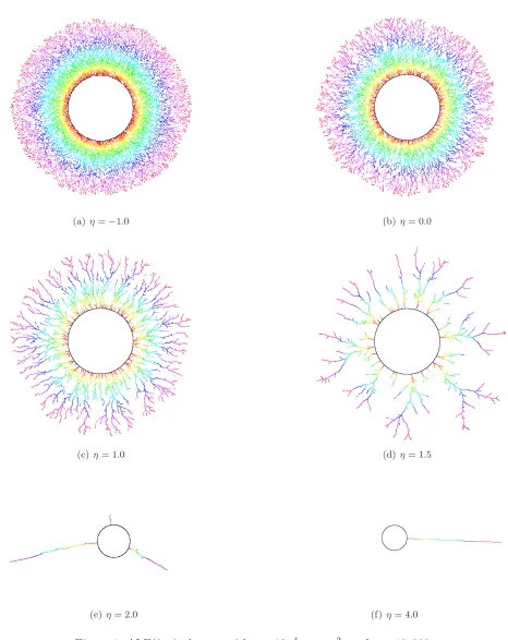
(a)η=−1.0 (b)η= 0.0

(c) η= 1.0 (d)η= 1.5

(e)η= 2.0 (f)η= 4.0

where Φk,j(z) =fk◦fk+1◦ · · · ◦fj(z).

In the ALE(0, η) model, each successive particle chooses its attachment point on the cluster according to the relative density of harmonic measure (as seen from infinity) raised to the power

η. As the highest concentration of harmonic measure occurs at the tips of slits, intuitively one would expect that for sufficiently large values of η each particle is likely to attach near the tip of the previous particle. In this paper we show that this indeed happens, and we identify the values ofη for which the above event occurs with high probability in the limit asc_→0. Figure 1 displays ALE(0, η) clusters for different values ofη.

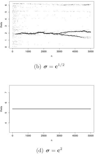
The limiting behavior of the model is quite sensitive to the rate at whichσ →0 asc→0. Figure

2 show how the angle sequences _{θk} in ALE(0,4) are affected by the choice of exponentγ when

regularizing byσ=cγ; this phenomenon is also observed by Hastings in [6] for a related model. In

[14], which deals with slow-decaying σ scaling limits in a strongly regularized version of HL(α), it

is shown that the scaling limits of the clusters are disks. By choosingσto decay sufficiently slowly

compared to c, once can prove that the corresponding scaling limits in ALE(0, η) are again disks, this is the topic of forthcoming work of Norris, Silvestri, and Turner. As we seek results which do not strongly depend on the choice of regularisation parameter, part of our objective is to identify the minimal value of η for which there exists some σ0 (dependent onc and η) such that, provided

σ< σ₀, with high probability each particle lands on the tip of the previous particle.

The following is the main result of the paper and shows that the ALE(0, η) model exhibits a phase transition at η = 1 in the genealogy of the growing cluster in the small-particle limit. See Theorem 16 for a complete statement and proof, in particular we give sufficient conditions on γ.

Theorem 1 (ALE(0, η) model). For ALE(0, η), let ΩN = Ωη,c,

σ

N be the event defined by

ΩN ={Particle j has parent j−1 for allj= 1, . . . , N}.

For each η > 1, there exists some γ = γ(η) such that if σ0 = cγ and if N =n(T) =⌊Tc−1⌋ for

some fixed T >0, then

lim

c→0

inf

0<σ<σ₀

P(ΩN) = 1,

whereas ifη <1, then for any N >1,

lim sup

c→0

sup

σ>0

P(ΩN) = 0.

In the case when η >1 and σ < σ₀, it follows that, for any r >1,

sup

t6T

sup

{|z|>r}|

Φ_n(t)(z)₋eiθ1_f

t(e−iθ1z)| →0 in probability as c→0,

and the cluster K_n(t) converges in the Hausdorff topology to a slit of capacityt at positionz=eiθ1_.

2.1 A related Markovian model

Observe that, for each k, we are free to specify the interval of length 2π in which to sampleθk, and

this choice does not have any effect on the maps Φn. It is convenient to choose to sample θk from

the interval [θk−1−π, θk−1+π). In this case, we can express the event as

ΩN =

(

sup

26j6N|

θj₋θj₋1|< βc

)

(a)σ=c1/4 (b)σ=c1/2

(c)σ=c(Note different spatial scale.) (d)σ=c2

Figure 2: ALE(0,4) angle sequences with c= 10−4 andn= 5,000, with varying regularizationσ.

(By definition, βc ∈(0, π) andei±β

c is mapped by the basic slit map to the base point of the slit

i.e.fc(e±iβ c

) = 1.) One of the main difficulties in analysing this event is that the distribution ofθk

conditional on_Fk−1 (as defined in (4)), depends non-trivially on the entire sequenceθ1, . . . , θk−1. In

this subsection, we introduce an auxiliary model for random growth in the exterior unit disk in which the sequence of attachment angles is Markovian. The auxiliary model is relatively straightforward to analyse and we show below that it exhibits an analogous phase transition to that described above. The remainder of the paper is concerned with examining how ALE(0, η) and the auxiliary model relate to each other.

Set Φ∗₀(z) =z and let _{Φ∗_n} be conformal maps obtained through composing

Φ∗_n=f₁∗_{◦ · · · ◦}f_n∗,

where eachf∗

k is a building block withck=c, and rotation angleθ∗khaving conditional distribution

with density

h∗_k(θ_|θ∗_k−1) = 1

Z∗

k−1

|fc′(k−1)(e

σ+i(θ−θ∗

k−1))|−η, k= 1,2,3, . . . . (6)

Here, we have set

Z_k∗ =

Z

T|

fc′k(e

σ+iθ

)_|−ηdθ

and suppressed the dependence on c, σ and η to ease notation. In order for the measure to be

this model is obtained by replacing the complicated (k₋1)th cluster map of ALE by a simple slit map “centered” at θ∗

k−1, and with deterministic capacity c(k−1).

For this model we obtain the following theorem: we again set n(t) =_⌊t/c_⌋.

Theorem 2 (Auxiliary model). Set σ0=cγ

∗

where

γ∗> η+ 1

2(η₋1)

Then

lim

c→0

inf

0<σ<σ₀

P(ΩN) = 1 ifη >1

lim sup

c→0

sup

σ>0

P(ΩN) = 0 ifη <1.

Furthermore, when η >1 and σ< σ₀, for any r >1,

sup

t6T

sup

{|z|>r}|

Φ∗_n(t)(z)₋eiθ∗1f_t(e−iθ∗1z)| →0 in probability as _c→0,

and the cluster Kn(t) converges in the Hausdorff topology to a slit of capacity tat positionz=eiθ

∗

1.

Remark. It can also be shown that limc→0inf0<σ<σ₀P(ΩN) = 1 when η = 1, provided σ0 → 0

exponentially fast asc_→0, but we omit the details here.

Proof. Since we can always rotate the clusters Kn by a fixed angle, without loss of generality,

we assume that the initial angle θ∗

1 = 0. As above, we choose to sample θk∗ from the interval

[θ_k∗₋₁₋π, θ_k∗₋₁+π). This means that we can writeθ∗_n=u2+· · ·+unwhere theukare independent

[₋π, π)-valued random variables anduk=θ∗k−θk∗−1 has symmetric distributionh∗k(θ|0).

First suppose η > 1. Then by (19) and Lemma 8 below there exists some constant A (which may change from line to line), depending only onT and η, such that

A−1(kc)1/2 < βkc< A(kc) 1/2_,

A−1

σ

1 + θ

2

σ2 −η/2

6h∗_k(θ_|0)6 A

σ

1 + θ

2

σ2 −η/2

for_|θ_|< βkc 2 ,

and

h∗_k(θ_|0)6Aση−1(ck)−η/2 for|θ|>βkc 2 .

Therefore

P

|uk|> βc

2

= 2

Z βkc

2

βc

2

h∗_k(θ_|0)dθ+ 2

Z π

βkc

2

h∗_k(θ_|0)dθ6A(ση−1c 1

2(1−η)+ση−1(ck)−η/2).

Hence, forη >1,

P(Ωc_N)6P

sup

26k6N|

θ∗_k−θ_k∗_−1|> βc

2

6 N

X

k=2

P

|uk|> βc

2

6Aση−1c− 1

2(η−1)c−1 −→0

Now suppose that η <1. Then, using Lemmas 8 and 9 and letting c_→0, we get

P(ΩN)6P(|θ2∗|< βc)6A

Z βc

2

0

cη/2dθ

(σ2+θ2)η/2

+

Z βc

βc

2

dθ

!

6Ac1/2 _−→0.

To show convergence of Φ∗

n(t)(z) to ft(z) for t < T whenη >1 andσ< σ0, by Proposition 3 it

is enough to show that sup_n6N|θ∗n| →0 with high probability asc→0. To do this, we write

θ_n∗ =

n

X

k=2

uk1_{|uk|<βc/2}+

n

X

k=2

uk1_{|uk|>βc/2}

and note that M∗

n =

Pn

k=2uk1_{|uk|<βc/2} is a martingale. Since θ ∗

n = Mn∗ with high probability,

convergence of sup_n6N|θn∗|to 0 follows from moment bounds in Lemma 9 together with standard

martingale arguments.

2.2 Overview of the proof of Theorem 1 and organization of the paper

The main idea for the proof is to show that the Markovian model of the previous section is a good approximation of the ALE(0, η) process. In order to do this one approach would be to try to argue that_|Φ′_n(eσ+iθ

)_|can be globally well approximated by_|(fθn

nc)′(e

σ+iθ

)_|. However, this seems difficult to make work to sufficient precision when evaluating the maps close to the boundary. Specifically, the map Φ′

n(z) has zeros (respectively singularities) at each of the points on the boundary of the

unit disk which are mapped to the tip (respectively to the base) of one of the slits corresponding to an individual particle. In contrast, for the map (fθn

nc)′(z), the points corresponding to tips and

bases of successive particles coincide and therefore the singularities and zeros corresponding to intermediate particles cancel each other out, leaving only a zero at the point mapped to the tip of the last particle and singularities at the two points which are mapped the base of the first particle (see Figure 3).

Interactions between nearby tips can be subtle and are in general hard to analyze [2]. Our strategy is instead to establish two properties of the distribution function hn(θ).

• The first is to show that near the tip of the last particle to arrive the derivatives are in fact very close and so for very small values ofθ,hn(θ+θn−1) can be well approximated byh∗n(θ|0).

• The second property is to show that hn(θ) concentrates the measure so close to θn−1 that

even though the probability of attaching to earlier particles is higher than for the Markovian model, ΩN still occurs with high probability, provided we now require

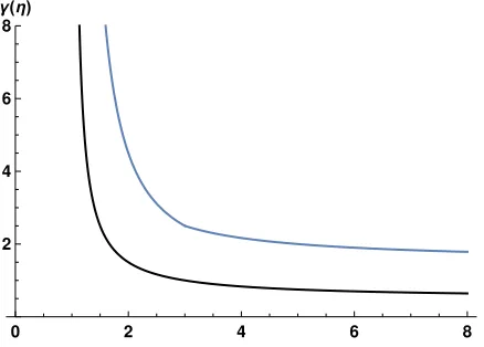
γ >

(

(2η2+η₋1)/[2(η₋1)2] if 1< η <3;

3η+1

2(η−1) if η >3

when regularizing byσ < σ₀ =cγ; see Figure 4 for plots of the lower bounds onγ and γ∗.

We now give a brief overview of the structure of the paper. In Section 3 we provide some back-ground information on the Loewner differential equation, which allows us to represent the aggregate maps Φn as solutions corresponding to a [−π, π)-valued driving process with equally spaced jump

Figure 3: Diagram illustrating the presence of zeros and singularities in the derivative at each successive particle tip and base in Φn(z) (left). These zeros and singularities are absent in fnc(z)

except at the tip of the final particle and base of the first particle (right).

In Section 4 we obtain estimates on the slit map used to construct ALE, as well as estimates on its derivatives. These latter estimates lead to moment bounds for [₋π, π)-valued random variables constructed from slit map derivatives. The arguments used are elementary in nature, and heavily use the explicit form of the slit map.

Section 5 contains most of the technical machinery needed for the proof. In this section, we obtain estimates on the distance between two solutions to the Loewner equation in terms of the distance between their respective driving functions in the case where we know that one of the solutions is a slit map. These estimates, which we believe may be of independent interest, enable us to obtain much more precise estimates than exist for generic solutions. In particular, our estimates give very good approximations when the conformal mappings are quite close to the boundary, whereas generic estimates blow up in this region. We perform this analysis by splitting the Loewner equation into radial and angular parts, and linearizing the resulting differential equations.

In Section 6, we use our estimates on Loewner derivatives at the tip and away from the approx-imate slit to show thathn(θ), the density function for thenth angleθn, has the required behaviour.

Then, similar arguments to those used in the proof of Theorem 2 are used to establish Theorem 1, but since_{θk}does not have a Markovian structure, there are further terms to control. Finally, we

discuss some extensions of our results, valid for certain instances of the ALE(α, η) model as well as related models.

Notation

0 2 4 6 8 η 2

4 6 8

γ(η)

Figure 4: Lower bounds on regularization exponents forALE(blue) and the Markov model (black).

3

Loewner flows

We shall make extensive use of Loewner techniques in this paper. Loewner equations describe the flow of families_{Ψt}t>0 of conformal maps of a reference domain inC∪ {∞}onto evolving domains

in the plane in terms of measures on the boundary. We only give a very brief overview here, and refer the reader to [17] and the references therein for a discussion of Loewner theory.

3.1 Loewner’s equation

Let _{µt}t>0 be a family of probability measures on the unit circle T, in this context referred to as

driving measures. Then the Loewner partial differential equation for the exterior disk,

∂tΨt(z) =zΨ′(z)

Z

T

z+ζ

z₋ζdµt(ζ), (7)

with initial condition

Ψ0(z) =z

admits a unique solution _{Ψt}t>0 called a Loewner chain. Each Ψt(z) is a conformal map of the

exterior disk onto a simply connected domain,

Ψt: ∆→Dt=C∪ {∞} \Kt

and at _∞ we have the power series expansion Ψt(z) = etz+O(1). The growing compact sets

{Kt_}t>0 are called hulls, satisfyKs(Kt fors < t, and have cap(Kt) =et fort>0, where cap(K)

denotes the logarithmic capacity of a compact set K_⊂C.

The limit functions appearing in Theorem 1 can be realized in terms of Loewner chains, and in fact have a very simple Loewner representation.

Example 1 (Growing a slit). Let µt=δ1, a point mass at ζ = 1. Then (7) reads

∂tft(z) =zft′(z) z+ 1

With initial conditionf0(z) =z, the solution has the explicit representation (viz. [20, p. 772])

ft(z) = et

2z

z2+ 2(1₋e−t)z+ 1 + (z+ 1)pz2_{+ 2(1−2e}−t_{)z+ 1. (8)}

The solution precisely consists of the slit maps ft: ∆→∆\(1,1 +d(t)], where

d(t) = 2et(1 +p1₋e−t_{)−2, t >0. (9)}

This means that the growing hulls areKt=D∪(1,1 +d(t)], the closed unit disk plus a radial slit

emanating from ζ = 1.

In this paper, we are mainly concerned with the case µt=δeiξt for some functionξt: (0, T]→R

and in that setting, we refer to ξtas a driving term.

The conformal maps arising in ALE(α, η) have the following simple Loewner representation. We first solve the Loewner equation with driving measureµt=δeiξt, where

ξt= n

X

k=1

θk1(Ck−1,Ck](t), (10)

with Ck = Pkj=1ck, and the angles {θk} and capacity increments {ck} given by (4) and (5),

respectively. Explicitly then, the Loewner problem associated with ALE(α, η) reads

∂tΨt(z) =zΨ′(z)

z+eiξt

z₋eiξt where Ψ0(z) =z. (11)

To obtain the composite ALE(α, η)-maps Φn described in Section 1, we evaluate the solution to

(11) at t=cn; thus

Φn= Ψcn, n= 1,2, . . . .

The random driving functionξtcan be viewed as a c`adl`ag jump process exhibiting a complicated

de-pendence structure encoded through angles and capacity increments. Whenα= 0, the dependence structure is only present in the distribution of the increments, as the jump times are deterministic, and equal to c_·k for k = 1,2, . . .. We emphasize that this is the main technical reason why the ALE(0, η) is easier to analyze then the general ALE(α, η) model or the Hastings-Levitov model HL(α).

Another version of Loewner’s equation arises in the setting of the upper half-plane

H=_{z_∈C: Imz >0_};

this is usually referred to as the chordal version of the Loewner equation. While the ALE model is defined in ∆, the half-plane formulas are simpler and are used in our analysis of the tip behavior, and so we give a quick overview here. The chordal version of Loewner’s equation with driving function ˜ξt: (0, T]→Rreads

∂tΨ˜t(z) =−Ψ˜′t(z)

2

z₋ξ˜t

, (12)

and we again consider the initial condition ˜Ψ0(z) =z. Solving (12), we obtain a family of conformal

maps ˜Ψt:H→ H\K˜t, mapping the half-plane to the half-plane minus a compact set and having

expansion ˜Ψt(z) = z−hcap(Kt)/z+O(1/z2) at infinity. The quantity hcap(Kt) = 2t is referred

Example 2 (Growing a slit in the half-plane). In the case where ˜ξt = 0, the chordal equation

becomes

∂tFt(z) =₋2

zF

′

t(z)

and we again obtain slit map solutions. In the half-plane, the corresponding closed formula is given by a substantially simpler expression than for ∆, namely

Ft(z) =

p

z2_{−4t, z∈H.}

3.2 Reverse-time Loewner flow

The Loewner equation (11) is a first-order partial differential equation, and in the ALE(α, η) model, it gives rise to a non-linear PDE problem since the driving measures depend on the mapsftvia their

derivatives. As is common in Loewner theory, we shall analyze solutions by passing to the backwards flow associated with (11): this essentially entails employing the method of characteristics to obtain an ordinary differential equation that describes the evolution at hand. See [17, 1] for detailed derivations and discussions.

Let T >0 be fixed. The equation for the backward or reverse-time flow in the exterior disk is

∂tut(z) =−ut(z)

eiΞt _+u

t(z)

eiΞt _−ut(z), (13)

where we define

Ξt=ξT−t, 06t6T.

Then, setting u0(z) =z, we obtain (see [17, Chapter 4])

uT(z) =fT(z)

whereftdenotes the solution to the forward equation (11) with driving functionξt. Note that this

holds in general only at the special time T.

In the half-plane, the corresponding reverse flow is governed by the equation

∂tht(z) =−

2

ht(z)₋Ξ˜t

, (14)

with driving function

˜

Ξt= ˜ξT−t

and initial condition h0(z) =z. For each T >0, we again have

hT(z) = ˜ΨT(z),

where ˜ΨT(z) is the solution to the Loewner PDE (12) for the upper half-place with driving function

˜

ξt, evaluated at time T.

3.3 Convergence of Loewner chains

Our strategy will be to argue that the driving functions arising in the ALE process are close, in the regime wheren_≍c−1, to the constant driving function ξt=θ1. We would then like to argue that

the resulting conformal maps are close. These kinds of continuity results have been established in several settings, see for instance [10, Proposition 3.1] and [13, Proposition 1], and [9] for a more systematic discussion.

Since the ALE driving processes exhibit synchronous jumps, it is natural to measure distances between them in the uniform norm_{k · k∞}. For T >0, we denote the space of piecewise continuous functions ξ: [0, T) _→ R endowed with this norm by DT. We consider the space Σ consisting of

conformal maps f(z) = Cz+_O(1), with C > 0 uniformly bounded, and we endow Σ with the topology of uniform convergence on compact subsets of ∆. We then view the conformal maps Ψt,

and hence the aggregate maps Φn, as random elements of Σ.

The following result is well-known, but we give a proof for completeness. (With additional work, one could obtain estimates on rates of convergence, but we do not pursue this direction here.)

Proposition 3. Let T > 0 be given. For j = 1,2 let Ψ_t(j),0 6 t 6 T, be the solution to the Loewner equation (7) with driving termξ(_tj). For every ǫ >0 there existsδ =δ(ǫ, T)>0 such that if _keiξ(1)₋eiξ(2)_k∞ < δ, then

sup

06t6T

sup

{|z|>1+ǫ}

Ψ

(1)

t (z)−Ψ

(2)

t (z)

< ǫ.

Proof. Fixs_∈[0, T] and consider the reverse-time Loewner equation (13). We letu(_tj)be the reverse flow driven by ξ_s(j₋)_t for 0 6t 6 s. Write W_t(j) = eiξs(j−)t_{. Taking the difference and differentiating}

H=u(1)₋u(2) with respect tot gives

˙

H₋Hv= (W(1)₋W(2))w,

where

v=v(t) = u

(1)_u(2)_−W(1)_W(2)_−(1/2)(u(1)_+u(2)_)(W(1)_+W(2)₎

(u(1)_−W(1)_)(u(2)_−W(2)₎

and

w=w(t) = (u

(1)_+u(2)₎2

2(u(1)_−W(1)_)(u(2)_−W(2)₎.

Since the flows move away from the unit circle, these expressions show that there is a constant A

depending only onT such that if_|z_|>1 +ǫthen for all 06t6s6T,

Rev(t)6A/ǫ2, _|w(t)_|6A/ǫ2.

Since H(0) = 0,

H(t) =

Z t

0

h

eRstv(r)dr(W(1)(s)−W(2)(s))w(s)

i

ds

and consequently, for a differentT-dependent A,

sup

{|z|>1+ǫ}|

Ψ(1)_t (z)₋Ψ(2)_t (z)_|= sup

{|z|>1+ǫ}|

H(t)_|6_kW(2)₋W(1)_k∞eA/ǫ2A/ǫ2.

Thus, we obtain convergence in law of conformal maps provided we can show convergence in law of driving processes. Note that in our main result we have convergence to a degenerate deterministic limit (modulo rotation). As is explained in [10, Section 4.2], we can strengthen the convergence that follows from Proposition 3 in this instance, and obtain convergence of Knwith respect to the

Hausdorff metric in ∆.

4

Analysis of the slit map

In our arguments, we shall need effective bounds on the building blocksfkmaking up the aggregated

map Φn = f1 ◦ · · · ◦fn, as well as on the derivatives fk′, in order to estimate moments of angle

sequences, among other things. In this section, we present both global and local estimates for the slit map.

An explicit formula for the slit mapft: ∆→∆\(1,1 +d(t)] was given in (8), while the length d(t) of the growing slit is given by (9). When performing estimates, it is sometimes helpful to view

ft as a composition of M¨obius maps with a slit map in the upper half-plane.

Define conformal maps mH: ∆→H={z∈C: Imz > 0}and m∆:H→∆ by setting

mH(z) =i

z₋1

z+ 1, z∈∆ (15)

and

m∆(z) =

1₋iz

1 +iz, z∈H. (16)

Ford >0, we check that

˜

fd(z) = 2

√

d+ 1

d+ 2

z2₋ d

2

4(d+ 1)

1/2

, z_∈H, (17)

maps the upper half-plane conformally onto the upper half-plane minus the slit 0, i_d+2d i. Note that (17) is a rescaling of the half-plane slit map from Section 3.

By following the image of the unit circle Tunder composition, and checking the trajectories of the point at infinity and the boundary point 1_∈∆, we verify that

ft=m∆◦f˜d(t)◦mH,

whered(t) is the explicit formula in (9). We note thatft(1) = 1 +d(t), and that one can compute

thatft(eiβt) =ft(e−iβt) = 1 for

βt= 2 arctan

d(t) 2p

d(t) + 1

!

. (18)

We shall refer to exp(iβt) and exp(−iβt) as the base points of the slit. In our scaling limit results,

we will make use of the facts that

βt

d(t) →1 and

d(t)

4.1 The half-plane

We start by analyzing the half-plane slit mapFt(z) =

√

z2_{−4tin detail near the tip. We note that}

F_t′(z) = z

(z2_−4t)1/2 and Ft′′(z) =−

4t

(z2_−4t)3/2.

Thus,F_t′ has a zero atz= 0, which gets mapped to the tip, and singularities at_±2t1/2, the points that are mapped to the base of the slit.

Lemma 4 (Near the tip, half-plane version). Let z=x+iy, where 0 6y 6t1/2 and _|x_|6 6

5t1/2.

Then

|Re[Ft(z)]|6y. (20)

and

7 10(2t

1/2_)6Im[F

t(z)]6

√

5 2 (2t

1/2_{). (21)}

Proof. By symmetry, it suffices to establish these bounds for x >0. The upper bound in (21) is obtained by evaluatingFt(z) atz=iy, right above the tip. We now establish the lower bound. Note thatx_7→Im[Fd(x+iy)] is decreasing on [0,6₅t1/2], and hence it suffices to estimate Im[Fd(6₅t1/2+iy)].

First, we compute

Ft 6 5t

1/2_+iy

4 = 16 25 2

(2t1/2)4 1 +425 64

y

2t1/2

2 + 25 16 2 y

2t1/2

4 !

.

Thus, setting y= 0, we obtain

Ft 6 5t

1/2_+iy

> 8 5t

1/2_.

Next,

argFt

6 5t

1/2_+iy

= π 2 − 1 2arctan 6 5 y

2t1/2

16 25 + (

y

2t1/2)2 ! > π 2 − 1 2arctan 15 16 y t1/2

,

and by our assumptiony/t1/261,

Im Ft 6 5t

1/2_+iy

> 8 5cos 1 2arctan 15 16

t1/2,

which leads to the lower bound in (21). A similar argument establishes (20). We first note that ReFd(x+iy) is increasing in x on [0,6₅t1/2] and use our expression for argFt to obtain

Re[Ft(6t1/2/5 +iy)]6

8 5t

1/2

1 + 8 y 2t1/2

2 1 4 sin 1 2arctan 15 16 y

2t1/2

631/43 4y,

where the last estimate (20) follows from the bound sin 1₂arctan(x)

4.2 The exterior disk

We now transfer back to the exterior disk, the setting of the ALE model, using the decomposition

ft=m∆◦f˜d(t)◦mH. To do this, we reparametrize and rescale the half-plane slit map to obtain

˜

f_d(t)(z) =C(t) z2₋ρ(t)21/2

,

where

C(t) = 2

p

1 +d(t)

2 +d(t) and ρ(t) =

d(t) 2pd(t) + 1.

We recall from (19) that ρ(t)/t1/2 _→1 as t_→0.

First, we describe the radial and angular effect of the building block map ft near the tip for

small values oft.

Lemma 5 (Near the tip, disk version). For_|z_{| −}16t1/2 and 0< t <1/20, and for argz6βt/2,

|ft(z)| −1>

1 10t

1/2 _{and |argf}

t(z)|62(|z| −1).

Moreover,

|ft(z)−1|

|ft(z)| −1 68.

Proof. Since _|ft(z)_|is non-decreasing in _|z_|, we may assume that _|z_{| −}1< ₁₀1t1/2. We first note that

mH(reiθ) =−

2rsin(θ)

r2_{+ 2rcos(θ) + 1} +i

r2₋1

r2_{+ 2rcos(θ) + 1}.

Using the fact that the real part is maximized on the unit circle, at argz=βt/2, together with the

identities sin(arctan(x)) = √ x

1+x2 and cos(arctan(x)) =

1 √

1+x2, we find that for 1< r <1 +

1 4t1/2

and _|θ_|6βt/2,

|Re[mH(reiθ)]|6

2 sin(βt 2)

2 + 2 cos(βt 2)

= ρ(t)

1 +p1 +ρ(t)2 6

1 2ρ(t).

We also have

Im[mH(reiθ)]>

r2₋1

r2_{+ 2r+ 1} >

r₋1

r+ 1 > 1

3(r−1), and by a similar argument to the one used to estimate the real part,

Im[mH(reiθ)]6

r+ 1

r2_{+ 2rcos(}βt 2) + 1

(r₋1) 6 2

3(r−1).

Thus, we can apply Lemma 4 to obtain

|Re[ ˜f_d(t)(mH(z))]6

2

3(|z| −1) and 7

10ρ(t)6Im[ ˜fd(t)(mH(z))]6 5

4ρ(t). (22)

To finish the proof, note that if w=x+iy_∈H,

m∆(x+iy) =

1₋x2₋y2 x2_{+ (1−y)}2 −i

2x

Fory > x, which is satisfied whenx= Re[ ˜f_d(t)(mH(z))] and y= Im[ ˜fd(t)(mH(z)],

|arg[m∆(x+iy)]|=

arctan

−₁ 2x −x2_−y2

6

arctan

−₁ 2x −2y2

6 2x

1₋2y2

and

|m∆(x+iy)| −1 =

((1₋x2₋y2)2+ 4x2)1/2

x2_{+ (y−1)}2 −1>

2y₋2x2₋2y2 x2_{+ (1−y)}2 >2

1₋2y x2_{+ (1−y)}2y.

We also have

|m∆(x+iy)−1|= 2

(x2+y2)1/2 (x2_{+ (1−y)}2₎1/2

so that

|m∆(x+iy)−1| |m∆(x+iy)| −1

6

1 +x_y2

1/2

(x2+ (1₋y)2)1/2

1₋2y 6

2 1₋2y.

The assertion of the Lemma now follows from the bounds in (22) and the fact that 2Im[ ˜f_d(t)(mH(z)]6 5

2ρ(t)6 34, by our assumption ont.

We now examine the derivative of the slit map in ∆.

Lemma 6. For0< t61 and 1<_|z_|62, we have

f_t′(z) =Ht(z)

et(z₋1)

(z₋eiβt₎1/2_(z−e−iβt₎1/2

(23)

where Ht(z) is holomorphic in z, has limz→∞Ht(z) = 1, and satisfies

A−1 6_|Ht(z)|6A

for an absolute constant A >0.

Proof. Since the slit map ft(z) solves the Loewner equation

∂tft(z) =zft′(z) z+ 1

z₋1

we have

f_t′(z) = z−1

z(z+ 1)∂tft(z). (24)

Differentiating the explicit expression (8) with respect tot, we find that

∂tft(z) = et

2z

z+ 1

p

(z+ 1)2_−4e−t_z

(z+ 1)p(z+ 1)2_−4e−t_{z+ (z+ 1)}2_−2e−t_z.

Inserting this into (24), we obtain

f_t′(z) =Ht(z) e

t_(z−1)

p

with

Ht(z) =

1 2z2

h

(z+ 1)z+ 1 +p(z+ 1)2_−4e−t_z−2e−t_zi_.

It remains to show that Ht is bounded above and below. But this follows immediately upon writing Ht(z) =z−1e−tft(z), whereft is the slit map itself. Finally, we verify that zt=eiβt solves

(z+ 1)2_−4e−t_{z= 0, and this leads to the factorization (z+ 1)}2_−4e−t_{z= (z−e}iβt_)(z−e−iβt_).

-3 -2 -1 0 1 2 3

1 2 3 4

-3 -2 -1 0 1 2 3

1 2 3 4

Figure 5: Plots of θ _{7→ |}f_t′(eσ+iθ

)_|. Left: σ = 0.0001 fixed, t= 0.01 (blue) and t = 0.1 (orange). Right: t= 0.01 fixed,σ= 0.0001 (blue) and σ= 0.02 (orange).

Plot with t= 0.1 and σ= 0.2 (black) shown in both pictures for comparison.

Our analysis of the ALE model will require local estimates on the derivative of the slit map. Representative graphs of howθ_{7→ |}f_t′(eσ+iθ

)_|varies with tand σ are shown in Figure 5.

Lemma 7. Let 0 < t61 and suppose _|z_{| −}1 6d(t). Then the derivative of the slit map admits the following estimates:

1. (Near the tip) For _|argz_|< 1₂βt,

A1et|

z₋1_|

d(t) 6|f

′

t(z)|6A2et|

z₋1_|

d(t) .

2. (Near the base) For _|argz_±βt|6 1₂βt,

A1et6|ft′(z)|6A2et

d(t)

|z_{| −}1.

3. (Away from tip and base) For _|argz_|> 3₂βt,

A1et6|ft′(z)|6A2et.

Proof. We treat the case _|argz_|< ₂1βt first. In light of the global bounds on the function Ht(z)

from Lemma 6, it suffices to estimate the square root expressions appearing in the denominator in (23). Noting that 0<_|z_{| −}16d(t), we have

|z₋eiβt_|=|elog|z|+i(argz−βt)_{−1| ≍ (log|z|)}2_{+ (arg(z)−β}

t)2

1/2

and hence

|z₋eiβt_|1/2_|z−e−iβt_|1/2 _≍d(t),

as claimed.

Near the base, the same reasoning as before shows that _|z₋1_{| ≍}d(t). On the other hand,

|z_{| −}16_|z₋eiβt_|6|elog|z|+i(βt+1₂βt)_−eiβt_|6Ad(t),

where the lower bound is attained when arg(z) =βt. Combining these bounds leads to the claimed

estimates for_|argz_±βt|6 β₂t.

On each fixed radius, the function v: arg(z)_7→

z−1

(z−eiβt)1/2_(z−e−_iβt)1/2

is decreasing on [

3 2βt, π],

with v(π) = (elog|z|+ 1)/((elog|z|+ cosβt)2+ sin2βt)1/2 >1. So in order to obtain the last set of estimates, it suffices to note that v remains bounded above and below as arg(z) _→ 3₂βt, by the

same arguments as before.

4.3 Moment computations

We now return to random growth models and present the moment bounds used in Section 2. As before, σ>0 is our regularization parameter, while η >0 is a model parameter.

For t >0, define the normalization factor

Z_t∗ =Z_t∗(η,σ) = Z

T|

f_t′(eσ+is

)_|−ηds. (25)

Lemma 8. Let 0< t <1 and suppose σ 6t1/2. The total mass Z∗

t satisfies the following.

• (η <1) There are constants A1 and A2 such that

A1 6Zt∗6A2. (26)

In particular, Z∗

t remains finite as σ→0.

• (η >1) There are constants A1 and A2 such that

A1d(t)ησ−(η−1) 6Z∗

t 6A2d(t)ησ−(η−1). (27)

In particular, if σ6t

η

2(η−1)_{, then Z}∗

t diverges as σ→0. Moreover, for η >1 we have the following estimates:

1. (Near the tip) For _|θ_|< βt 2,

A11

σ 1 +

θ

σ

2!−η/2

6 1

Z_t∗|f

′

t(e

σ+iθ

)_|−η 6A21

σ 1 +

θ

σ

2!−η/2

.

2. (Near the base) For _|θ₋βt|6 1₂βt,

A1σ2η−1d(t)−2η 6 1

Z_t∗|f

′

t(e

σ+iθ

3. (Away from the tip and base) For _|θ_|> 3₂βt,

A1ση−1d(t)−η 6 1

Z∗

t|

f_t′(eσ+iθ

)_|−η 6A2ση−1d(t)−η.

Proof. We begin by treating the case η <1. In light of Lemma 7, non-trivial global bounds on Z∗

t

from above and below follow immediately from the bounds for _|s_|> 3₂βt provided the contribution from (₋βt

2,

βt

2) is finite. Hence it suffices to estimate the integral

Z βt₂

−βt2

|f_t′(eσ+is

)_|−ηds_≍Ad(t)

Z βt₂

0

1

(σ2+s2)η/2ds,

where we have used that A1 <|eσ+is−1|/(σ2+s2)1/2 < A₂ fors,σ small. Next, we note that Z βt

2

0

1 (σ2+s2)η/2

ds6

Z βt 2

0

1

sηds,

and the latter integral is bounded for 0< t <1 since η <1. We turn to the caseη >1. Since the integralR

|f_t′(eis)_|−ηdsnow diverges due to the singularity at s= 0, it again suffices to estimate the contribution coming from_|θ_|< βt/2 in order to establish

(27). We have

Z βt 2

0 |

ft(e

σ+is

)_|−ηds6Ad(t)η

Z βt 2

0

(σ2+s2)−η/2ds

6Ad(t)ησ−η Z βt

2σ

0

σ(1 +u2)−η/2du

after a change of variables. SinceR∞

0 (1 +u2)−η/2duis now finite, the upper bound follows. Similar

reasoning together with the assumption that σ6t1/2 yields the lower bound on the integral. The

estimates on the normalized derivative for η >1 follow upon dividing through in Lemma 7 by the total massZ_t∗.

We now turn to moment bounds for η >1.

Lemma 9. Under the hypotheses of Lemma 8, we have, for each η >0, Z

T

θ 1 Z∗

t|

f_t′(eσ+iθ

)_|−ηdθ= 0.

Suppose x_∈(σ,βt

2). Then, for1< η <3, we have

A1x3−ηση−1 6 Z x

−x θ2 1

Z_t∗|f

′

t(e

σ+iθ

)_|−ηdθ6A2x3−ηση−1,

and for η= 3, we have

A1σ2log(xσ−1)6 Z x

−x θ2 1

Z∗

t|

f_t′(eσ+iθ

)_|−3dθ6A2σ2log(xσ−1).

For η >3, we have

A1σ26 Z x

−x θ2 1

Z∗

t|

f_t′(eσ+iθ

Proof. The statement thatR

θ_|f_t′(eσ+iθ

)_|−ηdθ= 0 follows immediately from symmetry of the func-tion θ_{7→ |}f′

t(e

σ+iθ

)_| for eachσ andt.

We turn to second moments, and deal with the parameter range 1< η63 first. By Lemma 8,

Z x

−x θ2 1

Z∗

t|

f_t′(eσ+iθ

)_|−ηdθ= 2

Z x

0

θ2 1 Z∗

t|

f_t′(eσ+iθ

)_|−ηdθ_≍σ2 Z x

0

θ

σ

2

1 + (σθ)

2η/2

dθ

σ .

Performing a change of variables, and assumingη <3, we obtain the integral

σ2

Z x

σ

0

u2(1 +u2)−η/2du=σ2 Z 1

0

u2(1 +u2)−η/2du+σ2

Z x

σ

1

u2(1 +u2)−η/2du

≍A1σ2+A₂σ2

Z x

σ

1

u2−ηdu

=A1σ2+A₂ 1

3₋ησ

2_x3−η_ση−3

=A1σ2+A₂x3−ηση−1,

as claimed. An obvious modification of the argument leads to bounds for η= 3.

Finally, we treat the caseη >3 and show that the second moment decays likeσ2 independently

of η. It now suffices to examine

Z

|θ|<x θ2 1

Zt|

f_t′(eσ+iθ

)_|−ηdθ_≍2σ2

Z x

σ

0

u2(1 +u2)−η/2du.

The integral on the right now converges sinceη >3, and in fact

Z ∞

0

u2(1 +u2)−η/2du=

√

π

4

Γ(η−₂3) Γ(η₂) .

To get the lower bound, we use the assumption 1 < x/σ to bound the integral from below. The

second assertion of the Lemma follows.

5

Estimates on conformal maps via Loewner’s equation

We now obtain refined estimates on the distance between solutions to the Loewner equation in terms of the distance between their driving functions, in the special case when the driving functions are close to constant. Generic estimates between conformal maps tend to blow up close to the boundary (as seen in, for example, Proposition 3).

As we wish to compare_|Φ′_n(eσ+iθ

)_|to_|(fθn

nc)′(e

σ+iθ

)_|whenσis typically much smaller than the

difference between the respective driving functions, we need bespoke estimates which behave well close to the boundary.

Suppose Ψt(z) is the solution to the Loewner equation (11). In this section, we compare Ψt(z)

and Ψ′_t(z) to ft(z) and ft′(z) in the case when ξ, the driving function of Ψ, is close to zero. For

fixed T >0, let

kξ_kT = sup t6T |

Writing uξ_t = r_tξeiϑξt, substituting into (13) and separating Re[(uξ

t + 1)/(uξt −1)] and Im[(uξt +

1)/(uξ_{t −}1)] we obtain the two differential equations

∂trξt =rtξ

(rξ_t)2₋₁

(rξ_t)2_−2rξ

tcos(ϑ ξ

t−ξT−t) + 1

(28)

and

∂tϑξt =−2

rξ_tsin(ϑξ_t−ξT−t)

(rξ_t)2_−2rξ

tcos(ϑξt−ξT−t) + 1

. (29)

In the special case when ξ _≡ 0 it is straightforward to see that if _|z_| > 1 and argz = 0, then

ϑ0_t = 0 for all t, whereas if _|z_| = 1 and _|argz_| > 0, then r0_t = 1 for all t < inf_{s > 0 : ϑ0_s = 0_}. Therefore, in these two cases, solving the pair of differential equations above reduces to solving a single ordinary differential equation, and we are able to obtain explicit solutions. We establish our bespoke estimates by linearising the differential equations around these explicit solutions.

In Section 5.1 we perform the analysis in the case when argz is close to 0, and in Section 5.2 we carry out the case when _|z_| is close to 1. We also obtain cruder estimates which apply in the intermediate regime between these two cases and will be used in the next section to “glue” the two results together.

5.1 Near the tip

In this subsection, we analyse Ψt(z) in the case when argzis close to zero. We begin by computing

an explicit expression for ft(r) when r > 1. Consider the reverse-time Loewner equations above

forz=r, withξt= 0 for all t. Since there is no dependency on T, we have thatft(r) =u0_t for all

t >0. From (28) it is immediate that ϑ0_t = 0 for all t >0. Substituting this into (28) we get

∂tr0_t =r0_tr

0

t + 1 r0

t −1

. (30)

Solving this gives

log

(r_t0+ 1)2r r_t0(r+ 1)2

=t

or

r_t0= (r+ 1)

2_et

2r 1 +

s

1₋ 4re−

t

(r+ 1)2

!

−1. (31)

Observe that ifr = 1, thenr0_t =d(t) + 1.

Now consider Ψt having general driving functionξt which is assumed to be small.

Proposition 10. There exists some absolute constant A such that, for all 1<_|z_|<2 and T >0

satisfying _kξ_kT +|argz|6A−1e−T(|z| −1), we have

|arg ΨT(z)−argz|6kξ−argzkT.

and

06r0_{T − |}ΨT(z)|6

AeT_kξ−argzk2

T

where r0_t is given by (31) with r=_|z_|. Hence A can be chosen so that

|ΨT(z)−fT(z)|6AeT(kξkT +|argz|).

Proof. First suppose that z= r0 ∈R and let uξt =rtξeiϑ

ξ

t be the solution to (13) starting from z.

We begin by showing that _|ϑξ_t|6_kξ_kT for allt 6T. Suppose that there exists some t1 6T such

thatϑξ_t1 >_kξ_kT. Since ϑξ0 = 0 andt7→ ϑ

ξ

t is continuous, there exists s1 < t1 such thatϑξs1 =kξkT

and ϑξ_t >_kξ_kT for allt∈(s1, t1] (take s1 = sup{t6t1 :ϑξt <kξkT}). Then sinceξT−t6kξkT for

all t6T, sin(ϑξ_{t −}ξT−t)>0 for allt∈(s1, t1]. Therefore, by (29),

ϑξ_{t1 −}ϑξ_s1 =₋2

Z t₁

s1

rξ_tsin(ϑξ_t−ξT−t)

(r_tξ)2_−2rξ

tcos(ϑξt−ξT−t) + 1

dt <0.

Henceϑξ_t1 < ϑξs1 =kξkT which contradicts our assumption that ϑ

ξ

t1 >kξkT. By symmetry, there is

also no t6T for whichϑξ_t <_−kξ_kT and hence|ϑξt|<kξkT for all t6T.

We now turn to r_tξ. Note that by (28), r0 6rtξ6rt0. Setδr(t) =rt0−rtξ and let

Tξ= inf_{t >0 :δr(t)>kξkT} ∧T.

Let

h1(r, x) =

r(r2₋1)

r2_{−2rcosx+ 1}. (32)

Then

dδr(t) dt =

dr0_t

dt −

dr_tξ

dt =h1(r

0

t,0)−h1(rtξ, ϑξt −ξT−t).

Suppose that t6Tξ. Set

H1(t) =h1(rt0−δr(t), ϑξt −ξT−t)−

h1(r0t,0)− ∂h1

∂r (r

0

t,0)δr(t) + ∂h1

∂x(r

0

t,0)(ϑξt −ξT−t)

=₋dδr(t) dt +

((r_t0)2₋2r0_{t −}1)δr(t)

(r_t0₋1)2 .

Here we have used

∂h1

∂r (r, x) =

r4₋4r3cosx+ 4r2₋1 (r2_{−2rcosx+ 1)}2

∂h1

∂x(r, x) =−

−2r2_(r2_{−1) sinx}

(r2_{−2rcosx+ 1)}2. (33)

Then, using (30),

d dt

r0_{t −}1

r0

t(r0t + 1) δr(t)

= r

0

t −1 r0

t(r0t + 1)

dδr(t)

dt −δr(t)

((r0_t)2₋2r0_{t −}1) (r0

t)2(r0t + 1)2

r0_t(r0_t + 1)

r0

t −1

= r

0

t −1 r0

t(r0t + 1)

dδr(t)

dt −δr(t)

(r0

t)2−2r0t −1

(r0

t −1)2

=₋ r

0

t −1

and hence

δr(t) =₋r

0

t(r0t + 1) r0

t −1

Z t

0

r0

s−1 r0

s(rs0+ 1)

H1(s)ds. (34)

By Taylor’s Theorem,

H1(t) =

1 2

δr(t)2 ∂2h1

∂r2 −2δr(t)(ϑ

ξ

t −ξT−t) ∂2h1

∂r∂x + (ϑ ξ

t −ξT−t)2 ∂2h1

∂x2

(r0

t−atδr(t),at(ϑ ξ t−ξT−t))

for someat∈(0,1). Now

∂2h1

∂r2 (r, x) =

4(r3cos(2x)₋3r2cosx+ 3r₋cosx) (r2_{−2rcosx+ 1)}3 ,

∂2h1

∂r∂x(r, x) =

4rsinx(2r3cosx₋3r2+ 1) (r2_{−2rcosx+ 1)}3 ,

∂2h1

∂x2 (r, x) =−

2r2(r2₋1)(r2cosx+r(cos(2x)₋3) + cosx)

(r2_{−2rcosx+ 1)}3 . (35)

We now bound these functions forr >1, seeking to reduce the singularities in the denominators as much as possible by exploiting simultaneous vanishing in the numerators. By using the fact that 2r(1₋cosx)6r2₋2rcosx+ 1, we have

∂2h1

∂r2 (r, x)

6 2(r

2_{+ 3r+ 4)}

(r₋1)3 ,

∂2h1

∂r∂x(r, x)

6 4rsin|x|(r+ 1)

2

(r₋1)4 ,

∂2h1

∂x2 (r, x)

6 8r

2_{(r+ 1)}

(r₋1)3 .

Observe that since _kξ_kT 6 A−1(r0 −1) 6 A−1(r0t −1), provided A > 2, we obtain the crude

estimates

(r_t0₋1)/26(1₋A−1)(r_t0₋1)6r0_{t −}atδr(t)₋16r_t0₋1,

and

sin_|at(ϑξt−ξT−t)|6|at(ϑξt −ξT−t)|63kξkT.

Therefore, using the fact thatt6Tξ, there exists some absolute constantA′ such that

|H1(t)|6

A′_kξ_k2_Tr0_t(r0_t + 1)2 (r_t0₋1)3 .

Substituting this bound into (34), we get

δr(t)6A′_kξ_k2_Tr

0

t(rt0+ 1) r0

t −1

Z t

0

r_s0₋1

r0

s(r0s+ 1)

r0_s(r0_s+ 1)2 (r0

s −1)3

ds

=A′_kξ_k2_Tr

0

t(rt0+ 1) r0

t −1

Z t

0

1

r0

s(r0s−1) ∂srs0ds

=A′_kξ_k2_Tr

0

t(rt0+ 1) r0_{t −}1 log

(r_t0₋1)r0

r0_t(r0−1)

6 10A

′_kξk2

TeT r0−1

Here we have used thatr0_t + 165et and thatxlog(1/x) is bounded by 1.

Therefore, taking A >10A′_{, we have δr(t) 6kξkT and hence T}ξ _{=T. It follows immediately}

that

|arg ΨT(z)|6kξkT and 06r0T − |ΨT(z)|6 A_kξ_k2

TeT

|z_{| −}1 . (36)

Now suppose that argz=θ₆= 0. It is straightforward to show that

ΨT(z) =eiθψT(|z|)

whereψT(z) solves the Loewner equation with driving function ξt−θ. It follows that

|ΨT(z)|=|ψT(|z|)| and arg ΨT(z) = argψT(|z|) +θ.

The result follows by replacing ΨT(z) by ψT(|z|) and ξt byξt−θin (36).

Finally, for the last part of the theorem, note that, if ξt ≡ 0, then clearly the conditions of

the theorem are satisfied. Therefore,_|fT(z)| −1 and argfT(z) also satisfy the above bounds from

which the second statement of the theorem follows.

We now turn to comparing the derivatives Ψ′_t(z) and f_t′(z).

Proposition 11. There exists some absolute constantA(taken to be at least as large as the absolute constant in Proposition 10), such that for all 1 < _|z_|< 2 and T >0 satisfying _kξ_kT +|argz|6 A−1e−T(_|z_{| −}1) we have

log

|Ψ′_T(z)_||z|(|z|+ 1)(r

0

T −1) r0

T(r0T + 1)(|z| −1)

6 Ae

T_kξ−argzk2

T

(_|z_{| −}1)2

and hence log Ψ′

T(z) f′

T(z)

6 2Ae

T_(kξk

T +|argz|)2

(_|z_{| −}1)2 .

Proof. Recall that ΨT(z) = uξ_T(z) where uξt(z) is the solution to (13) starting from uξ0(z) = z.

Hence Ψ′_T(z) =∂zuξ_T(z). Setyξ(t) =∂zuξ_t(z). Differentiating both sides of (13) gives

∂tyξ(t) =yξ(t)



 1−

2e2iξT−t

uξ_{t −}eiξT−t

2 

 .

Hence, usingyξ_{(0) = 1, we get}

yξ(t) = exp

   Z t 0   1−

2e2iξT−s

uξs−eiξT−s

2 

 ds



 

and so

|yξ(t)_|= exp

   Z t 0   1−Re

2

uξse−iξT−s ₋₁

2 

 ds





We evaluate the right hand side using the estimates from Proposition 10. Setting uξ_t =rξ_teiϑξt,

we have

Re 2

uξse−iξT−s−1

2 =

2((rsξ)2cos(2(ϑξs−ξT−s))−2rsξcos(ϑξs−ξT−s) + 1)

(rsξ)2−2rsξcos(ϑξs−ξT−s) + 1

2 .

Let

h(r, x) = 1₋2(r

2_{cos(2x)−2rcosx+ 1)}

(r2_{−2rcosx+ 1)}2 . (38)

Define δr(t) =r0_{t −}rξ_t as in Proposition 10. Then

log_|yξ(t)_|=

Z t

0

(r_s0)2₋2r_s0₋1 (r0

s−1)2

+H(s)

ds

= log

r_t0(r_t0+ 1)(r0−1)

r0(r0+ 1)(rt0−1)

+

Z t

0

H(s)ds,

where

H(t) =h(r_tξ, ϑξ_t−ξT−t)−h(rt0,0)

=₋∂h

∂r(r

0

t −atδr(t), at(ϑξt−ξT−t))δr(t) + ∂h ∂x(r

0

t −atδr(t), at(ϑξt−ξT−t))(ϑξt−ξT−t),

for someat∈(0,1). Now

∂h

∂r(r, x) =

4(r3cos(2x)₋3r2cosx+ 3r₋cosx) (r2_{−2rcosx+ 1)}3 ,

∂h

∂x(r, x) =

4rsinx(2r3_cosx−3r2_{+ 1)}

(r2_{−2rcos(x) + 1)}3 . (39)

These are the same expressions as in (35) and hence ifr >1, from the computation in the previous theorem, ∂h ∂r(r, x)

6 2(r

2_{+ 3r+ 4)}

(r₋1)3 ,

∂h ∂x(r, x)

6 4rsin|x|(r+ 1)

2

(r₋1)4 .

Hence, as in the proof of Proposition 10, for some absolute constant A,

|H(t)_|6 Ae

T_kξ−argzk2

Trt0(rt0+ 1)

(r0−1)(r0t −1)3 .

Using exactly the same argument as in Proposition 10, we obtain

log

|Ψ′_T(z)_|r0(r0+ 1)(r

0

T −1) r0

T(r0T + 1)(r0−1)

6 Ae

T_kξ−argzk2

T

(r0−1)2

.

The same bound holds for _|f_T′(z)_|and hence

log Ψ′

T(z) f′

T(z)

6 2Ae

T_(kξk

T +|argz|)2