Hierarchical descriptors for nonstationary 1 and 2 dimensional signal processing

http://wrap.warwick.ac.uk/

Calway, A. D. and Wilson, Roland, 1949- (1987) Hierarchical descriptors for

nonstationary 1 and 2 dimensional signal processing. University of Warwick. Department of Computer Science. (Department of Computer Science Research Report).

(Unpublished) CS-RR-108

Permanent WRAP url:

http://wrap.warwick.ac.uk/60804 Copyright and reuse:

The Warwick Research Archive Portal (WRAP) makes this work by researchers of the University of Warwick available open access under the following conditions. Copyright © and all moral rights to the version of the paper presented here belong to the individual author(s) and/or other copyright owners. To the extent reasonable and practicable the material made available in WRAP has been checked for eligibility before being made available.

Copies of full items can be used for personal research or study, educational, or not-for-profit purposes without prior permission or charge. Provided that the authors, title and full bibliographic details are credited, a hyperlink and/or URL is given for the original metadata page and the content is not changed in any way.

A note on versions:

UtinTftlf,r7 0..1VV

° 4

Research reoort 108

HIERARCHICAL DESCRIPTORS FOR NONSTATIONARY 1 AND 2 DIMENSIONAL

SIGNAL PROCESSING Andrew Caiway, Roland Wilson

(RR 108)

Abstract

The representation of signals with important local properties is considered. These signals have a degree of nonstationarity which is dependent upon the amount of localisation. Signal descriptors which seek to represent such signals must correspond in scale to the local properties in order to provide an efficient representation. A review is given of various methods that have been adopted. Although some of these have been used in specific applications, a general and computationally efficient representation is not available. A new descriptor is presented which seeks to fulfil this requirement. It - combines the time and frequency representations of a signal in an optimal way by using basis functions which are maximally concentrated in both domains. This corresponds to representing the local properties of the signal. The descriptor adopts a hierarchical structure which incorporates multi-resolution in both domains so that the required amount of localisation can be determined for a given signal. This enables the descriptor to be generally applied since it is consistent with the concept of a nonstationary signal. Results of initial experiments on the descriptor are presented and the report concludes with a discussion of future investigations.

Department of Computer Science University of Warwick

Coventry CV4 7AL

Hierarchical Descriptors for Nonstationary 1 and 2 Dimensional Signal Processing

Andrew Calway, Roland Wilson

Dept. of Computer Science, University of Warwick, Coventry

Introduction

Traditional signal descriptors, whether parametric [1] or non-parametric [2], have been based upon models which assume that the signal is stationary. A signal is defined as stationary if its properties are invariant to shifts in the time origin, ie the stationary signals f(t) and f(t+c) have the same properties for all values of c. Such signals can therefore be characterised by global informa-tion. Unfortunately, in many important applications, from speech processing to seismic analysis, these models have been found to be inappropriate.

Signals in these applications have local properties in the signal domain (eg time or space) that are important to the information that they convey. The signals therefore exhibit a degree of nonsta-tionarity which is dependent upon the localisation of this information. For example, in speech processing the transitions occurring at word boundaries are known to be significant, while in image processing the boundaries between regions of texture and uniform luminance are of per-ceptual importance. These are local properties contributing to the information contained in the signal.

If these signals are to be processed efficiently then they must be represented at a scale corresponding to their local properties, ie the resolution in the signal domain must be sufficient to enable these properties to be determined. This is why traditional stationary representations were inappropriate, they only considered global information (due to the assumption of stationarity) and ignored any local variation. A number of representations have been proposed which represent a signal at a scale corresponding to its local properties [3-7]. In particular, these are concerned with the local spectral content of the signal and they consequently combine time and frequency information. Although some of these methods have been used in specific applications, a general and computationally efficient representation is not available.

domains by varying these region sizes in a hierarchical structure. The motivation behind this is that within such a structure it should be possible to determine the scale of localisation in each domain required to optimally represent a given signal. This is why the descriptor can be generally applied: it can vary the scale according to the signal and is therefore consistent with concept of nonstationarity. The descriptor was originally proposed by Wilson [8] and each level of its struc-ture resembles the Gabor representation [3]. However, the basis functions used in the Gabor representation are replaced by functions which have inversion and computational advantages.

Of particular interest is the application of the descriptor to image processing. Recent work has indicated that this type of representation, which in its 2-d form combines spatial and spatial fre-quency information, is required to represent the inherent nonstationarity in images [9,10]. More-over, the hierarchical structure of the new descriptor can be regarded as a generalisation of the quad-tree or pyramidal representations which have achieved considerable success in recent years [11][12]. Such representations enable the image to be processed over a range of spatial resolu-tions, thus allowing the processing to take account of varying degrees of spatial localisation within the image. The new descriptor generalises this 'approach to include multi-resolution in both the spatial and spatial frequency domains.

The format of the report is as follows. Section 1 contains a review of the currently available time-frequency representations. The new hierarchical descriptor for 1-d and 2-d signals is then presented in sections 2 and 3. Some initial experiments are described in section 4: an implemen-tation example and a multi-level inverse. The report concludes with a discussion of future investi-gations into the properties of the descriptor.

1. Time-Frequency Signal Representations

Those representations considered have received the greatest interest in the literature: the Gabor representation, the short-time Fourier transform and the Wigner distribution. The definition and a brief description of each method is given, followed by a review of relevant work in the area.

1.1. The Gabor Representation

Since its proposal in 1946 by Gabor [3] in the context of information transmission, the represen-tation has received interest from authors in signal processing [13,14], vision research [15,16] and mathematical analysis [17]. Its importance as a time-frequency representation is therefore gen-erally accepted. However, doubts have been expressed by some authors over its mathematical properties and usefulness as a signal representation. Before considering these points a brief out-line and definition of the representation is given.

- 3 -

processing. This important principle was introduced by Gabor in his original paper [3], and states that a signal cannot be arbitrarily concentrated simultaneously in time and frequency. In the representation these elementary signals are centred at an array of points in the time-frequency plane. The expansion for a continuous signal f(t) is defined as :

f (t) = cki gki(t) (la)

k= i=

where the elementary signals gki(t) are defined as :

—Tc(t —kT

gki(t) = e a egint+9)

and

7c T = 2 = a:2-

The elementary signal is therefore a Gaussian-function with a variance of T2/27c centred about kT in the time domain and modulated with a frequency of / ( 4) is a phase constant ). Since the Fourier transform of gki (t) is given by :

G ki (CO) = (57 1 e --a(o)—1 47c e-i(cokr+o) ₍₂₎

a similar expansion, apart from a constant factor, exists for the Fourier transform of f(t). The representation is therefore symmetrically distributed in the time-frequency plane.

The elementary signals are concentrated at different points in the time-frequency plane. The coefficients of the representation therefore correspond to the local properties in the time and fre-quency domains of the signal f(t). The resolution of the representation is fixed in both domains and corresponds to the maximum that can be achieved simultaneously (due to the uncertainty principle ). Unfortunately, the elementary signals in equation (lb) are not orthogonal and it is therefore difficult to obtain the expansion coefficients. Gabor suggested a method of successive approximation to calculate the coefficients, however, as he readily admitted, it is not a satisfac-tory solution.

The representation has been extended in terms of generality and coefficient calculation by several authors. Lerner [13] dispensed with Gabor's fixed resolution and proposed an expansion in terms of more general signals. He used methods of orthogonalisation to obtain the coefficients of his new expansions. The idea of using different elementary signals was adopted by Landgrebe and Cooper [14] who proposed an expansion in terms of the prolate spheroidal wavefunctions [18-20] (cf section 2.1). Bandlimiting and timelimiting properties of these functions enable the coefficients of an expansion to be obtained without difficulty. These authors also applied the resulting expansion to the analysis of simple linear operators. Helstrom [21], and subsequently Montgomery [22], showed that exact continuous counterparts of the Gabor and Lerner expansions existed, resulting in the so called Gabor-Helstrom transform.

(lb)

The representation has received considerable interest in the field of vision research. Marcelja [15] suggested that a 2-d version is an appropriate model of the representation of images in the visual cortex. This received support from Pollen and Ronner [23]. Daugman [16] considered 2-d ver-sions of the Gabor elementary signals with an associated expansion and noted the similarity with the responses of simple cells in striate cortex of the cat.

Other workers have been concerned with obtaining the coefficients of the original Gabor expan-sion and on its resulting properties. Bastiaans [24] proved the existence of the expanexpan-sion and showed that the coefficients can be obtained via the following set of functions :

Xki(t) = ei (1r2r+0 (3a)

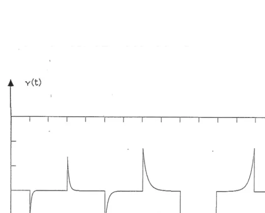
where the function 'y(t) is defined as :

-1 -3 _ 7C ta

70) = (20)-4- (k.„, e

a

I

Y

n>(+)-(-)±)

and the constant ko =1.85407468._ is the complete elliptic integral for the modulus 1Pri. The

function 'At) is shown in figure (1). The functions in equation (3a) are biorthonormal to Gabors elementary signals and the two are related by the following :

g (t) X„„, (t) dt = 5„,_k (4)

gk..i(t A.„„, (t2) = 6(t1-t2) (5)

/.—

where g,(t) are the Gabor elementary signals defined in equation (lb) and * indicates the

com-plex conjugate.. Equation (4) is the biorthonormal condition and the Gabor coefficients cn in

equation (la) are therefore given by :

cki = if (t) 41(t) dt (6)

The resulting expansion can be shown to be equal to f(t) by substituting the expression for the coefficients ca in equation (6) into the rhs of equation (la). Using equation (5) and the following identity :

6(tz-t 1) f dt 1= f (7)

then results in the equality of equation (la). This proves the existence of the Gabor expansion for an arbitrary signal.

However, although the above shows that a signal can be expanded in terms of the elementary sig-nals, the discontinuous and poor convergence properties of the biorthonormal functions in figure (1) means that the coefficients of the expansion are not easily found. Janssen [25] considered this problem and found that in general the expansion of equation (la) will not converge, ie :

- 5 -

Also, because of the discontinuous form of the function in figure (1), he predicted that the

calcu-lation of coefficients cki in equation (6) will, in general, be difficult.

The mathematical properties of the expansion therefore restrict a practical implementation. How-ever, this does not mean that the expansion is unsuitable for time-frequency signal representation. In particular, the work done in vision research indicates that the representation will continue to be used, since in this area its mathematical weaknesses are perhaps of less significance. Further, Gabors original idea of representing a signal in terms of signals which are maximally concen-trated in time and frequency may also be implemented by using alternative elementary signals. Examples include those proposed by Lerner [13] and Landgrebe and Cooper [14].

1.2. The Short-Time Fourier Transform

Of the time-frequency signal representations available, those utilising the short-time Fourier transform (SIFT) are the most well established. This is due to their extensive use in speech pro-cessing applications. The methods were first implemented using analogue techniques, including spectrographs for speech analysis and vocoders for efficient speech transmission [26]. Discrete versions were then developed which enabled these to be implemented efficiently and provide greater flexibility [27][28]. More recently the theory of the STFT has been generalised by Portn-off [4] and applied to signal representation and linear filtering operations. This work also showed that there is a similarity between the STFT and the Gabor representation.

The S11- of a discrete signal x(n) is defined as :

X (n ,co) = h (n —m)x(m) e-ic&" ₍₉₎

nt=

where co is a continuous frequency variable and h(n) is an appropriate window function. The STFT may be interpreted in two ways. First as the Fourier transform of x(n) weighted by the slid-ing window h(n). It then represents the spectrum of the signal viewed through the window

func-tion h(n). In this case, h(n) is known as the analysis window. Secondly, consider equation (9) as

the convolution relationship :

X (n ,o3) = h(n) (0„ x(m) (10)

where O„ denotes discrete convolution wit n, defined as :

z (n ,a)) = x (n ,u) „ y (n ,co) = y (n —m ,co) x (m ,co) (11)

fft

The S Ft. can then be interpreted as the output of a bank of bandpass filters with contiguous

fre-quency responses. For a given frefre-quency cop , the sequence X (n ,co p ) then corresponds to shifting

the spectrum of x(n) at cop to the origin and applying a low pass filter with impulse response

The synthesis of x(n) from its STFT is best considered in its general form proposed by Portnoff [4]. Other authors, notably Allen and Rabiner [29], have considered two separate synthesis for-mulas, however these were shown by Portnoff to be special cases of the general formula. This is given by :

x(n) = _rzr~f (n —r) X (r ,co) d co (12)

BTh

where f(n) is an appropriate synthesis filter. The equations (9) and (12) form a general STFT pair. A relationship between h(n) and f(n) can be derived which determines a condition such that x(n) can be exactly reconstructed from X (n ,co). By interchanging the order of integration and summa-tion in equasumma-tion (12) and noting that the integral is the short-time funcsumma-tion :

x(r ,n) = h(r—n) x(n) (13)

gives :

x(n) = f (n—r) h(r—n) x(n) (14)

r-

Therefore x(n) can be recovered exactly if and only if :

f (—m) h(m) = n1F (w) H (co) d co = 1 (15)

where F (co) and H (co) are the Fourier transforms of f(n) and h(n) respectively.

A discrete version of the STFT is considered by Portnoff [4]. In analogy with the continuous case, a general discrete STFT pair is defined as:

X (sR , Ulm) = h(sR—m) x(m) Cinifkm k = 0,1,....,M (16)

x (n) = m-1 f (n —sR) X (sR , kS2M) ejn' S2M = 27rtM (17)

This corresponds to samples of the continuous STFT at every R samples in time and Om radians in frequency. The condition that x(n) can be recovered from X (sR kf2m) is found by inserting the definition of X (sR , k SIM) into equation (17) and simplifying to give (Portnoff [4]) :

± f (n—sR) h(sR—n+pM) = 5(p) —0. < n <00 (18)

- 7 -

(18) with the relationship between the Gabor elementary signals and the functions required to determine the Gabor coefficients in equation (5). Thus, in the Gabor representation, the function

T(t) is the analysis filter corresponding to the Gaussian synthesis filter in the expansion of

equa-tion (1a).

When using the STFT, the form of the analysis and synthesis filters defined above is obviously important. From equations (9) and (10), it is clear that the analysis filter h(n) determines the reso-lution of the STFT in the time and frequency domains. A function which is concentrated in either domain will provide greater resolution in that domain. Since a function cannot be simultaneously concentrated in both domains (cf uncertainty principle, section 1.1), a trade off must be made between the resolution obtained in each domain. This has led to the use of wideband analysis, with h(n) concentrated in the time domain and narrowband analysis, with h(n) concentrated in the frequency domain [27]. A signal is analysed using one or several analysis filters with varying degrees of resolution in each domain. Furthermore, efficient methods of implementing the STFT using the fast Fourier transform algorithm have enabled adaptive methods to be used which alter the analysis window as a function of time [27].

Using the above techniques, the STFT has been successfully applied to speech processing appli-cations. This is because they correspond to adapting the analysis to the scale of the local proper-ties of the signal and are therefore able to represent the varying degrees of nonstationarity encountered in speech signals. However, at present, these techniques have been applied in a somewhat ad hoc manner and have not been unified into a single representation which can be generally applied. Therefore, although the STFT can be implemented efficiently, it does not fulfil the requirement for a generally applicable nonstationary representation.

13. The Wigner Distribution

This is a generalised correlation function that indicates the distribution of a signal over the time-frequency plane. It was introduced in 1933 by Wigner [30] in the field of quantum mechanics. However, its application to signal processing received little attention until recently. Its reintro-duction into the signal processing literature was largely due to a comprehensive set of papers published by Claasen and Mecklenbrauker [5-7]. They presented the definition, properties and variations of the distribution for both continuous and discrete signals. In theory, the distribution has a potentially superior resolution to the other representations considered here. However, to implement the distribution a modified version must be used which results in removing this advan-tage. This problem, and a further complication with the discrete version, has resulted in limited application of the distribution.

The Wigner distribution (WD) of a continuous signal f(t) is defined as :

where * indicates conjugate complex. 'The Will at time to is the Fourier transform of a function

which corresponds to taking symmetrical correlation products about to . As with the other

representations, it is concerned with the local properties of a signal. However, unlike the other representations, the definition in equation (19) does not involve an external window function but is dependent only upon the signal of interest. In this form, the distribution would therefore have a superior resolution in both time and frequency.

Unfortunately, this advantage is removed when the implementation of the WD is considered. As can be seen from equation (19), the determination of the WD for each value of t requires the sig-nal to be known for all time. Also, the Fourier integral for all frequencies of interest needs to be computed. Therefore, to enable implementation, a variation of the WD must be employed which uses a sliding window function to truncate the signal. This is known as the pseudo Wigner distri-bution (PWD). A set of weighted functions f, (t) is defined :

f i(t) = f w (t-t) (20)

where w(t) is the window function. Noting that the WD of a function g (t) = f (t) m (t) is given by :

Wg (I'm ) = 7 Wf (t ,11) Wm (t ,(0-11)

dil

The WD of the functions f ,(T) is then :

Wf,(T,co) = -2T 1Wf (T,T1) Ww (T—t ,co—ri) del (22)

In equation (22), the parameter t indicates the position of the window function wrt the signal f (t).

Centring the window function about the point where the WD is to be evaluated, ie T=1, equation

(22) then becomes :

147f (t ,co) = WL(T,co)] = j Wf (t,i) Ww (0,ori) di (23)

The function 1,17f (t,o)) is the pseudo Wigner distribution. Both equations (20) and (23) indicate the loss of resolution in time and frequency encountered when the WD is implemented using the PWD.

A property of the WD that must be considered is that it is a bilinear functional of the signal. In other words, the WD of the sum of two signals is not simply the sum of the WD's of those sig-nals. The relationship is derived from equation (19) :

Wf+g (t 40) = Wf(t,w) W9 (t ,w) + 2 Re Wf ,g (t ,C0) (24)

where Wf ,g (t,co) is the cross-WD of the signals f(t) and g(t). This property will present

- 9 -

The discrete WD is not so well defined as its continuous relation. The following definition is adopted :

Wf (n ,8) = 2 ki f (n+k) f (n—k) evue (25)

where n is the discrete time variable and 0 the continuous frequency variable. The problem

asso-ciated with the function Wf (n ,e) is that it is periodic with period it, due to the factor 2 in the

exponent. Since the spectra of discrete time signals have a period of 27r, W.) ( n ,0) will contain

aliasing contributions due to the true WD 'folding back'. As suggested by Claasen and Mecklenbrauker [6], the aliasing problem can be avoided by ensuring that the discrete signal spectra are zero for radial frequencies greater than n, either by oversampling the continuous sig-nal (wrt the Nyquist rate) or interpolating the origisig-nal discrete sigsig-nal. The aliasing problem is also removed when the distribution is considered for analytic signals, the spectrum of which vanishes for negative values. The problem is considered in a separate paper by Claasen and Mecklenbrauker [31].

Other authors have also published work on the distribution, most notably Janssen [25] and De Bruijn [32]. The former considered the mathematical properties of the continuous WD and com-pared them to the Gabor representation. He concluded that the convergence properties are more predictable for the WD (cf section 1.1) and that greater resolution could be expected from the continuous WD. The distribution was considered in relation to the uncertainty principle by De Bruijn, who also provided a lucid description of the nonstationary signal analysis problem.

Recent applications, although limited, have occurred in optics [33] and vision research [10]. Of particular interest here is the application to vision by Jacobson and Wechsler [10]. They used a 2-d version of a PWD, known as a composite PWD, to present a model for the operation of sim-ple and comsim-plex cells within the striate cortex.

2. A Hierarchical Nonstationary Signal Descriptor

2.1. Notation

The data used is assumed to be discrete time samples of the signal being analysed and form a

finite sequence x(0) ,x (1) , , x(N-1). Where appropriate a vector representation will be

adopted and then linear operators are indicated by upper case letters while vectors are given lower

case. In particular, the Fourier transform operator is indicated by F and its inverse by F+, see

Wil-son [8]. All shift operators for a finite sequence are cyclic (modulo N).

2.2. The Basis Functions for the Descriptor

The extent to which the time and frequency representations of a signal can be combined is limited by the uncertainty principle [3]. This states that a signal cannot be simultaneously concentrated in both domains to an arbitrary extent. Therefore, since the descriptor seeks an optimal time-frequency combination, it is based upon signals with minimum uncertainty, ie those which are maximally concentrated in both domains. Examples include the Gabor functions [3] and the pro-late spheroidal wavefunctions (PSWF) [18-20]. The difference between these functions being the type of measurement used for the concentration of the signal in a each domain. The Gabor func-tions are derived from a standard deviation measurement, while the PSWF's maximise the energy in a finite interval of one domain while truncating in the other. It is the latter that are used as a basis for the descriptor, primarily because they can be defined to be exactly bandlimited (unlike the Gabor functions) which has computational and inversion advantages.

The discrete form of the PSWF's are the finite prolate spheroidal sequences (FPSS), Wilson [8]. They can be defined by the following eigenvalue problem :

B riTs gk = ?Lk gk (26)

where Ts is the truncation operator defined as :

ts j = Sij 0. <S

= 0 S i

and B n is the bandlimiting operator defined as :

B0 = F+TriF

The eigenvalue corresponds to the eigenvector gk,

(27)

(28)

which is the required finite prolate

spheroidal sequence. The notation g(x ;S ;C2) is adopted for such a sequence.

It can be shown that the best eigenvector in terms of energy concentration is that corresponding to

the largest eigenvalue of equation (26) [8]. The resulting FPSS, go (x ;S ;-S2), is exactly

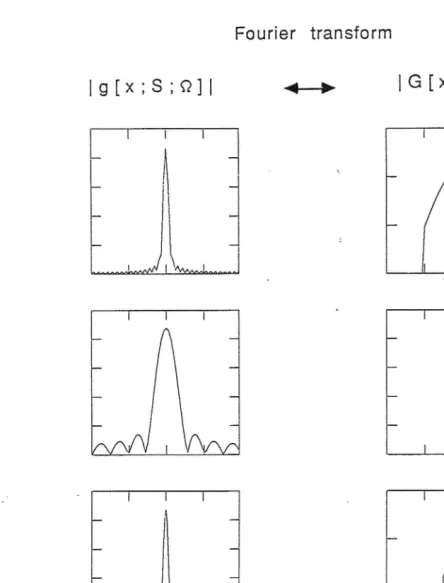
bandlim-ited to a region of size fl and optimally concentrated in a temporal region of size S. Examples of

considered.

23. The Descriptor

For a finite sequence f ( x ) of length N =2n, the descriptor consists of n+1 levels, each having N samples, as in figure (3). On the bottom level, level 0, is the original sequence. A given level above, level 1 say, is divided into 21 frequency domain sets each containing 2A-1 temporal sam-ples. These sets represent disjoint bands covering the frequency domain. Each set is produced by convolving f ( x ) with the FPSS go (x ; 21 ; ), and subsampling by a factor equal to 21 . The FPSS is centred within the frequency band represented by the set. On higher levels, the number of frequency sets successively increase by a factor of two, the number of temporal samples within each set decreasing by the same factor. The top level is just the discrete Fourier transform of the sequence f ( x ).

For an intermediate level 1, the 1-d descriptor is defined as :

N-1 i 2= aux,

h(x ,u) = f (Sx—x') go (x';S ; ) e'71- (29)

Ox <S2 <S S =2! = 2n-1

The following points should be noted :

(i) A single level of the descriptor is a time-frequency representation of the original sequence which resembles the Gabor representation, with the elementary signals replaced by the FPSS's.

(ii) The hierarchical structure contains varying degrees of resolution in each domain, ranging from the original signal to its Fourier transform. Therefore, by selecting a single level or combination of different levels, it should be possible to determine a representation of a sig-nal corresponding to the scale of its local properties. In this respect the descriptor resembles a unified version of the wideband and narrowband analysis techniques used in the applica-tion of the short time Fourier transform (cf secapplica-tion 1.2).

(iii) Each time-frequency sample on a level represents the information of the original sequence contained in its respective time interval and frequency band.

(v) The resolution in each domain, on a given level, is determined by the number of frequency sets and temporal samples within those sets.

(vi) Since the generation of the frequency sets on each level of the descriptor correspond to the simple filtering operation in equation (29), the descriptor can be efficiently implemented using FFT methods.

(vii) Due to the sampling rates adopted and the use of the exactly bandlimited FPSS's, each level of the descriptor can be readily inverted (see appendix).

3. Extension to the Two-Dimensional Case

The descriptor is readily extended to 2-d and it is for this case that an example is provided in sec-tion 4. Definisec-tions and addisec-tional considerasec-tions are dealt with in this secsec-tion.

3.1. The Two-Dimensional Basis Functions

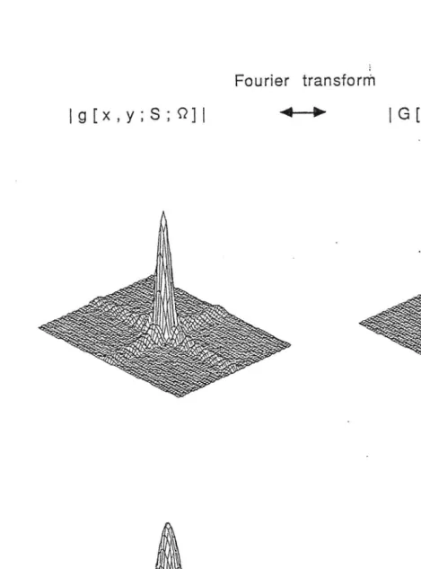
A combination of the spatial and spatial frequency information for a discrete image is required. Once again the uncertainty principle, applied to 2-d [34], is the limiting factor and thus the descriptor is based upon 2-d minimum uncertainty sequences. Both the Gabor functions [16] and the FPSS's [8] have 2-d forms, the latter being used for the same reasons as in the 1-d case. The FPSS's can be defined in both cartesian and polar separable forms [8], however, since in the cartesian separable case the eigenvectors are simply the Kronecker product of the 1-d problem, this will be adopted to provide a convenient definition of the descriptor. Examples of some carte-sian separable FPSS's are shown in figure (4). Note that the polar separable descriptor will be a straightforward extension of the cartesian separable case.

3.2. The Two-Dimensional Descriptor

For an image f ( x , y) of size N x N, N = 2n , the cartesian separable descriptor has a similar

form to that of the 1-d case, see figure (5). There are n+1 levels each having N xN samples, the

bottom level is the original image and the top level is its 2-d Fourier transform. On an intermedi-ate level 1, there are 221 spatial frequency domain sets, each containing 22(n-1) spatial samples.

For an intermediate level 1, the cartesian separable descriptor is defined as :

N -1 N -1

h(x ,y ,u ,v) = f (Sx—x' ,Sy—y') go (x' ,y';S ;.(2) e• 2n •+ vy

xr (30)

0..x <S1 0<_u <S S = 2'

0 <S SI =

where the 2-d FPSS, go (x ,y ;S ;g2), is given by :

-13-

It should be clear that the properties noted in section 2.3 for the 1-d descriptor are equally valid for the 2-d case. In addition, note that the hierarchical, multi-resolution structure of the 2-d descriptor is a generalisation of the quad-tree or pyramidal representations which have received considerable interest in image processing [11].

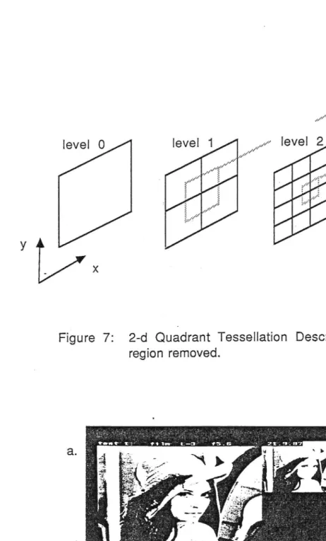
3.3. Spatial Frequency Tessellations

The sets on each level of the 2-d descriptor corresponds to disjoint regions covering the spatial frequency domain. Since the levels are 2-d, the descriptor may adopt a variety of tessellations for these regions. Allowing for the natural restriction of symmetry to these tessellations, there are still many possible types that could be considered. Obviously, any such tessellation should be implementable using the FPSS 's and on this criterion one can classify tessellations into those corresponding to cartesian separable or polar separable implementation, as in figure (6). Note that it may be necessary to introduce additional spatial frequency sets on each level of the descriptor to achieve a given tessellation, however, apart from the extra computation, this should not present problems. The advantages/disadvantages of these tessellations are as yet unknown. However, as noted by Wilson [8], the choice will depend upon those features within an image which are regarded as important, eg if orientation is important then the polar separable configurations would be appropriate. It is also clear that the computational advantage gained by using cartesian separ-able tessellations would also have to be considered. For the work done so far in this project, the cartesian separable quadrant tessellation descriptor in figure (5) has been used.

4. Experimental Results

It is now appropriate to consider the results of some preliminary experiments - an implementation example and a 'multi-level' inverse algorithm.

4.1. An Example

Results of implementing the 2-d descriptor are presented. A frequency domain tessellation corresponding to the simple quadrant in figure (5) was adopted. However, a lowpass region, equal in size to each quadrant, was removed before calculating each level. The FPSS correspond-ing to the respective level was used as the lowpass filter, ie :

d(x ,y ) = N-1 (-1)( f+r) go (x' ,y';S ; 12 ) f (x—x' ,y—y') (32)

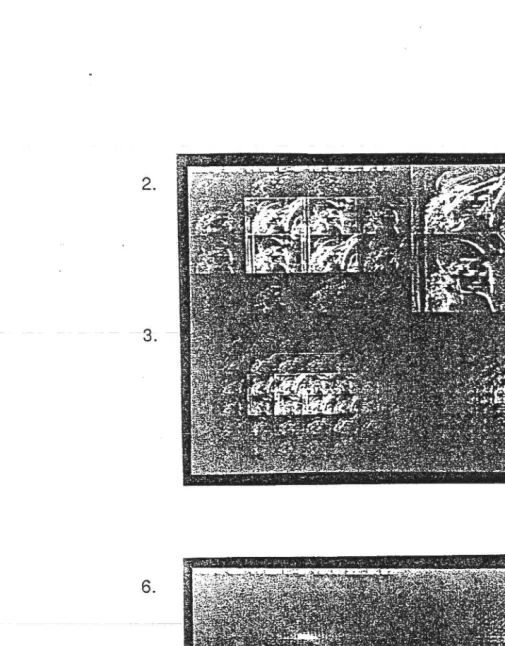
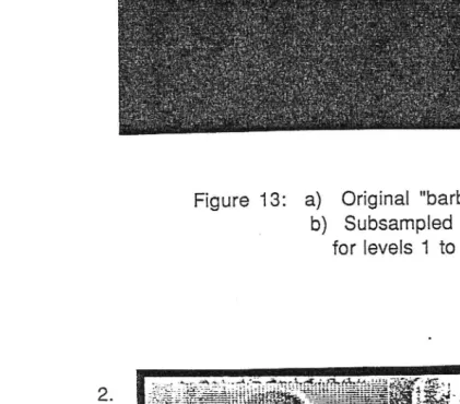
the image in figure (8a) which consists of 256 x 256, 8-bit grey level pixels. The lowpass filtered images, subsampled by a factor 21 , for each level of the descriptor are shown in figure (8b).

A level of the descriptor, given by equation (30), can be interpreted as being located on a finite

4-d lattice, with coordinates x y ,u ,v. Within such a lattice, h (x ,y ,u ,v ), it is possible to

define separate spatial and spatial frequency vector spaces, ie :

h (u ,v) = h (x ,y ,u ,v ) h (x ,y) = h (u ,v ,x ,y)

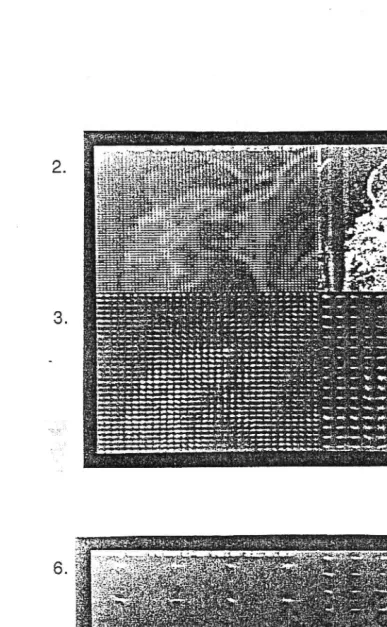
For a level 1, the spatial vector space is of dimension 22(n-1), while the spatial frequency vector space has dimension 22' . To overcome the difficultly in displaying a 4-d lattice, either of these vector spaces can be used to display the descriptor coefficients. The complex magnitude values for both spaces on all levels of the descriptor are shown in figures (9) and (10). Each space is displayed on a 2-d lattice formed by the other two coordinates. For example, on level 1, there are

2"-1 x 2!" spatial frequency vectors, of dimension 22', located at points in the original image

separated by 24-1 samples. The vector spaces obviously convey different types of information and hence the one used to display the descriptor will depend upon the relevant property.

4.2. A Multi-Level Inverse Algorithm

In the appendix it is shown that a given level of the descriptor is readily inverted. However, since it is intended that within the hierarchical structure of the descriptor an optimum representation of a signal should exist, it is relevant to consider_ inversion using coefficients from a combination of levels.

For convenience, the algorithm is defined in terms of the 1-d descriptor, extension to 2-d is straightforward. It is shown in the appendix that a sequence, represented by the vector f, can be recovered from the descriptor vector h , at level 1, using the following formula :

f= M X F+ G-1 F h M= 2' (34)

where G-1 is the inverse FPSS frequency domain operator defined in equation (A8). In the multi-level inverse algorithm, coefficients are selected from a number of intermediate multi-levels of the descriptor using a given criterion (as yet undefined). A pseudo-inverse, 11, is then produced for each of these levels using the selected coefficients, all the other coefficients being set to zero, ie :

= M F+ G-1 F is (35)

where the selected coefficient vector, h , is given by :

= C h

and C is the selection operator :

Cpq = 5pq iff selection criterion true at hp

= 0 else

(33)

(36)

- 15 -

The multi-level inverse,

f ,

fi

(38)

L 1 <L2 0 <L1 L2 < n

Although, by definition, the resulting signal will not be an exact reconstruction of the original signal, it is reasonable to suggest that if the selection criterion is such that the selected coefficients are an optimal representation of the image (in the sense of local properties), then an acceptable result will be obtained.

An experiment to test the above procedure was performed on the descriptor presented in section 4.1. Using levels 1 to 4, a threshold criterion was used to select coefficients from the levels, ie the selection operator, C, was defined as :

Cpq = 3pq I p I. ?. threshold

= 0 else

Since in such a simple technique there is no decision concerning the preference of one level over another, the threshold value was varied between levels to ensure a uniform distribution of coefficients. The results for various threshold values, affecting the number of coefficients selected, are shown in figures (11 a-11c).

There are two sources of error in the results. First, the 'ringing' effects in the vicinity of lines and edges, particularly when fewer coefficients are used, is caused by aliasing. This occurs because the selection of coefficients from each level corresponds to a further subsampling operation on the frequency domain sets. Since these sets are a result of sampling at the Nyquist rate (cf appen-dix), their spectra 'fold back' due to this additional sampling. This is why the 'prewhitening' descriptor structure was adopted (cf section 4.1), the large lowpass contribution in images tends to produce high frequency aliasing components when the additional subsampling is applied. Since these effects are particularly unpleasant to the viewer, any method which reduces the con-tribution of the lowpass region (such as prewhitening) is beneficial. Secondly, the 'blotchiness' is caused by non-uniform distribution of the selected coefficients over the image, ie some areas have a greater contribution from the coefficients than other areas. It should be possible to reduce this effect by using a selection criterion which ensures a uniform distribution.

As would be expected, the better results are obtained for the inversion when a larger number of coefficients are used. This corresponds to increasing the sampling rate and thus reduces aliasing. It should also be noted that the threshold selection criterion used would not necessarily yield an optimum representation and therefore better results may be possible by using an alternative cri-terion. Determining such a selection criterion will form part of the future work to be done on the descriptor (cf section 5.1).

To provide a comparison for the results, the image in figure (8a) was filtered using a filter with a lowpass Gaussian frequency response (figure 12) which results in a similar number of coefficients to the multi-level inverse example in figure (11c). The filtered image is shown in figure (11d). By comparing this 'blurred' image with the 'sharper' multi-level inverse result, it is clear that the descriptor is able to represent the local properties of the image, such as lines and edges, as well as the lowpass' contribution.

5. Conclusions and Further Work

The problem of representing signals with important local properties has been considered. Representations which have received the greatest interest in the literature were reviewed, how-ever it was shown that none of these combined sufficient generality and computational efficiency. A signal descriptor which seeks to fulfil this role was then described. Initial experiments using the descriptor were presented, an implementation example and a multi-level inverse procedure, for which acceptable results were obtained. The following sections describe the further work that is intended to be done using the descriptor.

5.1. Analysis of the Descriptor

This is concerned with determining an optimum representation of a. signal from the hierarchical structure of the descriptor. It will be necessary to establish the relationship between coefficients in the descriptor and then decisions can be made concerning the best coefficients to be used. In particular, the relationship between coefficients of different levels will be of interest and what consistent (or inconsistent) information between these levels indicates about the signal being analysed.

This work will be useful in image analysis problems where areas of texture and the location of lines and edges are to be determined. By knowing the relationship between levels, ie knowing what consistency and inconsistency imply, it will be possible to make decisions such as 'the tex-ture in region A is optimally classified at level k, while the best estimate of its position is at level

k-1'. These ideas will therefore utilise the multi-resolution structure of the descriptor.

-17-

5.2. Operations on the Descriptor

The intention in this work will be to define and implement linear operators on the descriptor. At the top and bottom levels this will correspond to familiar filtering operations. However, at inter-mediate levels it will be possible to define new types of operations.

Consider the spatial frequency vector space defined in section 4.1, ie :

h (x ,y) = h (u ,v ,x ,y) (40)

It is then possible to define a general operator for this level, G, (x ,y), to transform the vector space

h (x ,y) to the space d (x ,y):

d ( x , y ) = x; y; Gi(x' ,y') h (x—x' ,y—y') (41)

Note that a similar general operator could be defined for the complete descriptor.

As an example consider a filtering operation applied to a level of the descriptor. This can be defined in terms of the following convolution relationship :

d(x ,y ,u ,v) = x;; g(x' ,y' ,u ,v ) h(x—x' ,y—y' ,u ,v ) (42)

y

0 < X < 2(n-1) 0 < u <2' 0 < y < 2(n-i) 0 < v <21

where d(x ,y ,u ,v ) is the filtered descriptor level and g(x ,y ,u ,v) is the filter impulse response wit x and y, and the filter frequency response wit to u and v. When vector notation is used, equation (42) is equivalent to equation (41), with the general operator, G, (x , y ), given by :

gpq (x ,y)= 8pg g(x,y,u,v) p = 14 21 (43)

By extending the general operator to include non-diagonal components, more complex operations on the descriptor may be defined. It is the intention of future work to implement and investigate these, as well as the simpler filtering operations

Appendix

A sequence can be recovered exactly from a level of its hierarchical descriptor. To show this, it is convenient to use vector and linear operator notation. The original sequence is represented by the vector f . Relevant definitions and useful operators are considered first.

For the sequences f ( x ) and g (x) with discrete Fourier transforms 7( u) and T( u ) , the

con-volution theorem is defined as :

f(x) Ox g(x) <—> 7(u) .1(u ) (Al)

where <—> indicates the Fourier transform and O. the discrete convolution defined in equation (11).

Useful operators include the circular shift operator, S :

Spq = 5(p+1)q (p+1) modulo N _(A2)

and the subsampling operator, MD :

mdpq 15pq

=0

p = r M

else Or <NIM (A3)

The following identities should be noted :

F mD F+ = S11" (A4)

wr

11

Also, define the FPSS frequency domain operator, GI(u), as :

gipq ( u) = fo (p—u S2 ; M ;SI) 5pq M = 21 SZ = 2"-1 (A6)

where io( u;Ai;t1) is the Fourier transform of go (x ;M ; S2) . The subscript / and the index u

will be dropped when appropriate to avoid confusion. Note that the operator G is a bandlimiting

operator, ie :

S-"IGFf=GFf (A7)

The inverse G operator, G-1 , is defined as :

G-1 G = Sun Ttl I (A8)

where I is the identity operator.

For an intermediate level 1, the descriptor is given by the convolution and subsampling

relation-ship in equation (28). Using vector notation for the descriptor, ie :

- 19 -

and equation (Al), this can be rewritten as :

h = mD F+ G F f M = 2! (A10)

Forming the operator F+ G-1 F and operating on h gives :

F+ G-1 F h = F+ G-1 F MD F+ G F f (All)

Using equations (A4), (A5) and (A7) this becomes :

F+ G-1 F h= F+ G-1 G F f = 714- F+ Tn F f (Al2)

Therefore, the original sequence is exactly recovered using the following relationship :

f = M F+ G-1 F h (A13)

References

1. Koopmans, L.H.

The Spectral Analysis of Time Series. New York, Academic Press, 1974.

2. Thomson, D.J.

Spectrum Estimation and Harmonic Analysis. Proc. IEEE, 70, 1055-1096, 1982.

3. Gabor, D.

Theory of Communication. Proc. ME, 93, 26, 429-441, 1946.

4. Portnoff, M.R.

Time-Frequency Representation of Digital Signals and Systems Based on Short-Time Fourier Analysis.

IEEE Trans. ASSP, ASSP-28, 55-69, 1980.

5. Claasen, T.A.C.M and Mecklenbrauker, W.F.G.

The Wigner Distribution - A Tool for Time-Frequency Signal Analysis. Part I: Continuous-Time Signals.

Philips J.Res., 35, 217-250, 1980.

6. Claasen, T.A.C.M and Mecklenbrauker, W.F.G.

The Wigner Distribution - A Tool for Time-Frequency Signal Analysis. Part II: Discrete-Time Signals.

Philips J.Res., 35, 276-300, 1980.

7. Claasen, T.A.C.M and Mecklenbrauker, W.F.G.

The Wigner Distribution - A Tool for Time-Frequency Signal Analysis. Part III: Relations with other Time-Frequency Signal Transformations.

Philips J.Res., 35, 372-389, 1980.

8. Wilson, R. and Spann, M.

Finite Prolate Spheroidal Sequences and Their Applications I, II. IEEE Trans. PAMI, accepted for publication.

9. Granlund, G.H.

-21-

10. Jacobson, L. and Wechsler, H.

A New Paradigm for Computational Vision Based on the Wiper Distribution. Technical Report, University of Minnesota, 1982.

11 Adelson, E.H. and Burt, P.J.

The Laplacian Pyramid as a Compact Image Code. IEEE Trans. Corn., COM-31, 532-540, 1983.

12. Spann, M. and Wilson, R.G.

A Quad-Tree Approach to Image Segmentation which combines Statistical and Spatial Information.

Patt. Rec., 18, 257-269, 1985.

13. Lerner, R.M.

Representation of Signals.

Lectures on Communications Systems Theory, Baghdaddy, E.J. ed., New York, McGraw-Hill, 204-242, 1961.

14. Landgrebe, D.A. and Cooper, G.R.

Two-Dimensional Signal Representation Using Prolate Spheroidal Functions. IEEE Trans. Comm. Elec., 30-40, 1963.

15. Marcelja, S.

Mathematical Description of the Responses of Simple Cortical Cells. J. Opt. Soc. Amer., 70, 1297-1300, 1980

16. Daugman, J.G.

Uncertainty Relation for Resolution in Space, Spatial Frequency, and Orientation Optim-ised by Two-Dimensional Visual Cortical Filters.

J. Opt. Soc. Amer., 2, 1160-1169, 1985.

17. Janssen, A.J.E.M.

Gabor Representation of Generalised Functions. J. Math. Anal. & Appl., 83, 377-394, 1981.

18. Slepian, D. and Pollak, H.O.

Prolate Spheroidal Wavefunctions, Fourier Analysis and Uncertainty I. BSTJ, 40, 43-64, 1961.

19. Landau, H.J. and Pollak, H.O.

20. Landau, H.J. and Pollak, H.O.

Prolate Spheroidal Wavefunctions, Fourier Analysis and Uncertainty III. BSTJ, 41, 1295-1336, 1962.

21. Helstrom, C.W.

An Expansion of a Signal in Gaussian Elementary Signals. IEEE Trans. Inf. Th., IT-12, 81-82, 1966.

22. Montgomery, L.K.

A Generalised of the Gabor-Helstrom Transform. IEEE Trans. Inf. Th., IT-13, 344-345, 1967.

23. Pollen, D.A. and Ronner, S.F.

Spatial Computation Performed by Simple and Complex Cells in the Visual Cortex of the Cat.

Vision Res., 22, 101-118, 1982.

24. Bastiaans, M.J.

Gabor's Expansion of a Signal into Gaussian Elementary Signals. Proc. IEEE, 68, 538-539, 1980.

25. Janssen, A.J.E.M.

Gabor Representation and Wigner Distribution of Signals. Proc. ICASSP, California, 1984.

26. Flanagan, J.L.

Speech Analysis, Synthesis and Perception. New York, Springer-Verlag, 1965.

27. Oppenhiem, A.V.

Speech Spectrograms using the Fast Fourier Transform. IEEE Spectrum, 7, 57-62, 1970.

28. Portnoff, M.R.

Implementation of the Digital Phase Vocoder using the Fast Fourier Transform. IEEE Trans. ASSP, ASSP-24, 243-248, 1976.

29. Allen, J.B. and Rabiner, L.R.

-23-

30. Wigner, E.

On the Quantum Correction for Thermodynamic Equilibrium. Phys. Rev., 40, 749-759, 1932.

31. Claasen, T.A.C.M and Mecklenbrauker, W.F.G.

The Aliasing Problem in Discrete-Time Wigner Distributions. IEEE Trans. ASSP, ASSP-31, 1067-1072, 1983.

32. De Bruijn, N.G.

Uncertainty Principles in Fourier Analysis.

Inequalities, O.Shisha. ed, New York, Academic Press, 1967.

33. Bastiaans, M.J.

Wigner Distribution Function and its Application to First Order Optics. J. Opt. Soc. Amer., 69, 1710-1716, 1979.

34. Wilson, R. and Granlund, G.H.

The Uncertainty Principle in Image Processing. IEEE Trans. PAMI, PAMI-6, 758-767, 1984.

35. Blackman, R.B. and Tukey, J.W.

The Measurement of Power Spectra from the Point of View of Communications Engineer-ing - Pt 1.

L

r

)

1

1

-4.5

-3.5

-2.5

-1.5

-0.5

0.5

1.5

2.5

3.5

4.5

t

Fourier transform

Ig[x;S;NI -41--0. IG[x;S,S2]1

N=64

S=2

Q =32

N=64

S=8

Q=8

N=128

S=4

Q=32

N=128

S=16

Q=8

i 1 1

1 1 1

1 1

1

1 I 1 1 I

r

Level 0 : original sequence frequency

time

Fourier transform

Ig[X,y,S;Q]l 1G[x,y ,S;Q]l

2-d Car tes ian Sep a ra b le De sc rip to r.

11.11MA

INIM111

c

C,

X

•

FC

= >. F. H .,•••

ti3 a '-<- H

= Ht cr;

C < ... >, 0

G P.1 0 Le 0

...3 0 0

0 < F. •-• = 7.

L.) .-1 in C.

0 •••-' <

CZ. ....' 0

H < H o a

LI : 5...-

C-7 ...2 Lt. ■••••• La a.

= 0 H F.

C <

0• U-•

H

= al

LII < H

Lt.1 H ,-, C

ra.1 LL1 0 CI 00

01 < H H

H F. =

0 Lt3 E. Z cr) <

< C, <C C

-6. m .-1 >, H

level 1 i level 2 ...level n

Y A

lowpass regions

Figure 7: 2-d Quadrant Tessellation Descriptor with lowpass region removed.

a. b.

Figure 8: a) Original "girl" image.

3. 4.

6.

7.

• ••• ...A...a • 4.. • •

• ,

•••••••• .• • • •

••••••••••••••• ••• 41, ••• • •• 111-•• MI. • •• • IV •• •■• • ••• ;.•• ••••••• • ••••••••,•••• • IRO. •■ ••••••••• • •••• . •

ale• • ON. ••••••••••••••••••• • • • .••••••• ••• • ••• ••• ••••• 1•4••• •• ••• ••••••• • •11••••••••• •• • •

• ••• •••• •••••• ••• ••• • • • •• ••■

Va. ■••••••••,-•7`,.."-..41'' 6 ;UV. •••-•• ' 16 ,•■•••■■•-••oirtwo, •••,,•••1 •••■•••••••• v••r•n••••••• • •••■••••••• - • - •

If: O. .116 "woc..Nti

••••••••*••••••••••• • •••••-- _{••• •••• • V. 4.•}

- - •.r..11 •-••••••••••■•••••••• • •■••■•• ••. • • ••••••`. dm, •015,20,,,

‘,...,•••••...z • • • • • •••4 •• .,•••••••.. .Z.12

a••••••••••••os•••••••+o • • , ..•••••

- — e.

Vet Ne:•....e

••■••■••■••■••••■••••w•.•••,••-•.••••• • •

2.

3.

1.

4.

-

#t • t7.4:t't•k

c.

d.

Figure 11: Multi-level inverse results. Number of coefficients:

a) 3N21 4 b) N2/ 2 c) N2/ 4

d) Filtered image corresponding to N2/ 4 coefficients.

a.

b.

2.

3.

Figure 13: a) Original "barbara" image.

b) Subsampled lowpass filtered images

for levels 1 to 4.

. - - . , - , - - 4 . ' — .- 4. — - I - . • • 4 • , 3 - . -1, - . l. A. ,•! ic ,

.:::= 1 ...,

•

k. rer• , 1,.3.,

r...derl, .. 5 •

1 4 ..".

-11.- • . .fir

',... I *-

4

12 _. . _{' d-:;=.41 wir-}

- .. • .

•

&..-... .... -.- .--.

.... _,

-L'_.

.,..

..._ •

:A ...--*--- ....-. - ...---....—.---.-. ... -- - . .9, 1. ...s. -... -4.- .. -11. ,II. 40. AB ... _{41.-....- ...--...} ....".•••••■■••••---.... —, ... -.--1.-.1.,440:11. Mt OW '441.:11r.410,....4#4 _{_.} ••...--...-..-■■■••-...-■.•-••••••••■••---•-■- ,-,. ... ,... -,,-...-...4. -No 71,-

,...., _...-...--..,.-1•-• ...- •-•-•*--"--..."-..." et.

-

. •••••, •• •• ..•••ddr .101...••• •••• • • .••••••••••••••••.' * * -' * - '''..."."...."...:••• • 4'. ' 4.-••••'•It•' •••• ■ • ., .. ...., .5...%•11•414

....*"... "'"*." '. ... ••••• 40 -■••••••,•••.. ••• . , • ,-..., ...,...,..41 , . ..,, ... • • ...••••••••••,1•.••• ••••• • • • . • ••••••••••••.:•• ; • :

-

• or ■■■••••... 4. ••• •■ N...

&N.., --.. •••■■••■"...• .••••• •... . ' ." ...* ...""'" ''', .. ' :, , .".., ...,„ ...Y... ...- *I. . , ....' '111. ..e ...'•.1 '..li...:. 44 ..., -....1",e.S... . ...^. 4 - ...•••“•••••• .% .• .

amoaaa'a ,-... A. .,..•••■••••,.. .••••• .• ..{..• •• "" •••••• .• ..-... ••• ...1..., ... ,ow., • . ...c.•...).., ,...' ...i. 1 .1. -.4...44.,... ,...4- .S...7 ,...`. '''.. A ..• }M... ■ ••• ... ••••■■•■•■•■• 4.0..,

....--...,- ...- ... ...-...—=:-... .7... ..._{. A....,...,..c.„ ."... Of:, . ■". .d., ....,, ...4...1....0.6410 ,,}

. '

' ...'''''..."...'-' .. ..'-',.'..w ...",..."),../...t

6"::::::;".. _---. mr....v...r...

... N.-...- ....:... , #...now, ... ... ... • ,..1roge,011**am.ormslayr

..."..'"' "... ' ""*.• ...r

••■■■■•■■•■ • _{...-,.. ...d..0.511~~4.1011.1.1} 4

ilb."...snw -

. •

4.