Magnetic self assembly in 3 dimensions at the macro scale

Magnetic Self-assembly in 3 Dimensions at the Macro Scale.

Pieter Kamp

Thesis BSc Assignment Advanced Technology,

Transducer Science and Technology,

University of Twente,

Enschede,

Netherlands,

[email protected]

Committee:

Miko Elwenspoek, chairperson

Leon Abelmann, member

Gert Jan Koster, external member

L´

eon Woldering, supervisor

Abstract

Contents

1 Introduction 2

2 Literature Study 4

2.1 Control Parameters of Self-assembly . . . 4

2.2 Prior Art . . . 6

3 Self-assembly in an Airbubble Agitated Watercolumn 8 3.1 Structured particles . . . 9

3.2 Binding force . . . 11

3.3 Environment . . . 14

3.4 Driving force . . . 17

3.5 Boltzmann distribution . . . 17

3.6 Self-assembly kinetics . . . 19

4 Results and Discussion 21 4.1 Reynolds number of tetrapod . . . 21

4.2 Interaction of 2 magnetic spheres . . . 22

4.3 Average height of particles . . . 23

4.4 Interaction of two tetrapods . . . 26

4.5 Self-assembly with 8 tetrapods . . . 30

4.6 Lifetime of configurations with 8 tetrapods . . . 32

5 Conclusions and recommendations 34 5.1 Conclusions . . . 34

5.2 Recommendations . . . 34

A Characterization of particles 41

B Magnetization measurements 42

C Tetrapod structures 46

1

Introduction

Self-assembly is the intriguing process mastered by the flora and fauna. Most natural systems are the product of self-assembly. Self-assembly is the process in which a disordered system orders itself trough a stochastic driving force into a functional pattern or system. Self-assembly is present at all scales, from the smallest molecules to the greatest stellar systems. Mankind is researching this smart building method for different reasons. First there is the understanding of life itself, self-assembled biological cells function as long as they dissipate energy. If the cell does not dissipate energy it dies. We would like to know how and why the universe became what it is today. We have limited understanding about the fundamental principles of self-assembly, therefore it is worth researching. Besides understanding life there is the engineering part of self-assembly which may prove to be a future direction in enabling new technology. Self-assembly may offer the path to more complex systems, look for example at the complexity of a human being as a working system. Even bacteria are far more complex compared to the most intricate system thought of and produced by man. Therefore, self-assembly as a production process may enable new technologies.

Self-assembly enables the production of ordered states of matter which otherwise would not be possible. Examples of this are: photonic crystals and three-dimensional microstructures [Elwenspoek 2010]. Charac-teristics of different materials could be combined to engineer materials with new possibilities. For instance: metallic particles inside a soft polymer matrix would give a conductive but compliant material. Metal parti-cles inside a ceramic matrix would give a ’metal’ with very high yield strength. Units with negative poisson ratio could be self-assembled or piezoelectric elements with a much larger range of deflection could be created [Elwenspoek 2010]. Current production of microstructures is done by lithography, which is intrinsically a, 2D, planar production technology. Self-assembly allows for 3D production technologies [Whitesides 2002]. Finally there is the trend of miniaturization of products: the production lines for increasingly smaller prod-ucts are going towards a limit. Serial pick-and-place processes will have difficulties coping with the decreasing size of the products as the pick-and-place robots have to become increasingly larger. Self-assembly may offer an economic and efficient alternative [Zheng 2005].

This thesis focuses on non-molecular self-assembly. Researching non-molecular self-assembly is interesting for several reasons. Firstly non-molecular particles are often easier to produce compared to particles at the micro or nano scale. The particles used in this research are 3D printed. Secondly self-assembly at the macro-scale is more easy to observe, no expensive apparatus like atomic force microscopes or scanning tunnelling microscopes are needed. Finally the lessons learned from the macro scale situation could be extrapolated to the micro domain.

The goal of this research is to research under which conditions three-dimensional self-assembly into a diamond-like structure occurs in an aqueous system in which tetrapods fitted with disk-shaped magnets are agitated by a flow of air bubbles. The results of this research may offer a deeper understanding of the fundamentals of self-assembly and may proof to be useful when scaling down to sub-micron scale.

2

Literature Study

Self-assembly is multidisciplinary: biologists, chemist, physicists, engineers all have a different view on self-assembly. In order to get some clarity on the subject of self-assembly it is helpful to provide a framework to define and analyse self-assembly. However this is not the only or absolute framework possible, because of the diversity of self-assembly. Furthermore a short review of relevant prior art is given.

One definition of self-assembly is: ”Processes involving pre-existing components which are reversible, and can be controlled by proper design of the components and controlling boundary conditions of the system. These processes lead to self-organization into desired patterns and functions through stochastic process”. This definition helps us to choose control parameters of self-assembly.

2.1

Control Parameters of Self-assembly

In each self-assembling system a particular set of features is recognizable. This helps to analyse the system and also provides control parameters to ’steer’ the self-assembly. The control parameters of self-assembly will be explained by characterizing an experiment done by Stambaugh et al. in which spheres fitted with long and short magnets where put in a container. The container was agitated vertically for a period of time and the assembled patterns were observed. [Stambaugh 2003].

We consider four control parameters for self-assembly: structured particles, a binding force, an environ-ment and a driving force, see table 2.1. These control parameters are proposed by Pelesko [Pelesko 2007]. The parameters will be discussed below.

Control Parameter Structured Particles Binding force Environment Driving force

Table 2.1: Control parameters in a system of self-assembly.

The structured particles are the component of the system which form the structure and perform the self-assembly. Self-assembly can be guided by engineering the particles in such a way that mostly the desired structures will form. In the experiment by Stambaughet al. the structured particles are spheres, fitted with long and short magnets. They are engineered in such a way that they can move freely within a container. In the case of this bachelor assignment the particles are printed plastic structures fitted with magnets. 3D Printing enables us to obtain particles with an arbitrary shape, in this case tetrapods and spheres.

Figure 2.1: Photograph of two tetrapods fitted with 5 mm magnets and 5.5 mm caps forming a dimer. Also visible are air bubbles which agitate the system. This is crucial for self-assembly as a driving force.

Figure 2.2: Photograph of four tetrapods equipped with 5 mm magnets and 5.5 mm caps forming a ring like structure. The air bubbles provide a driving force by agitating the system.

The environment provides boundary conditions on the movement of the particles. The boundary condi-tions can be provided by: the physical edge of the system in which self-assembly takes place, the medium in which the particles are, and by external forces acting on the system and its particles. External forces may be gravitational, electromagnetic fields or otherwise. In the experiment of Stambaugh et al. the environment is the enclosure of the container in which the spheres self-assemble. There are no immediate external forces influencing the process. Gravity is not influencing the process because the particles have very little room to move vertically. In this bachelor assignment the environment consists of: the water in which the particles are submersed, the tube in which the water is contained, gravity pulling the particles down, and the upward flow of water provided by the airflow and waterflow.

Driving forces in self-assembly are the forces which ’drive’ the process towards local energy minimization. Driving forces agitate the system, providing energy and mobility to the particles. These driving forces preferably are stochastic. Examples of driving forces are: thermal noise, physical oscillation of the system, and a fluctuating electromagnetic field. In the experiments of Stambaughet al., the container which holds the spheres is shaken vertically providing energy to the system to rearrange itself. Kinetic energy is provided to the particles in the vertical direction, but because of the restriction in vertical motion the particles start to move at random in the non-restricted horizontal plane of environment. In this bachelor assignment the driving force is the flow of air through the column, see figures 2.1 and 2.2. The air bubbles agitate the particles, analogue to thermal motion at the sub-micron scale. The difference between thermal motion, or Brownian motion, at the sub-micron scale and the air bubble flow at the macro scale is that thermal motion is fully random. The air bubble flow has a component which is directed upwards because of the difference in density between air and water. In the horizontal plane the agitation by air bubbles probably is presumed to be random. Another driving force is provided by the drag on the particles by the upward flow of water. We think that the agitation by air bubbles is sufficiently random to perform self-assembly.

self-assembly is by using a template which restricts the initial binding orientation.

Self-assembly generally can be divided into static or dynamic self-assembly. Static self-assembly processes drive towards a local energy minimum. In dynamic self-assembly processes ordered states only exist when the system is dissipating energy. For example: a living cell only works and lives when it is dissipating energy. If it stops dissipating energy, it dies. In this bachelor assignment the attracting forces are generated by permanent magnets. If the airflow or distorting energy agitating the particles is stopped, the energy provided to the system is taken away. The magnetic attraction however does not cease to exist and the particles will still stick together, the structure is ’frozen’. Therefore the self-assembly in this situation is static. Particles tend to find the lowest state of magnetic energy locally available.

Self-assembly is only successful if there is a potential energy difference between the assembled and dis-assembled states. Otherwise the energy needed to assemble two particles is equal to the energy needed to disassemble the two particles again. Statistically this is not an advantage for the process of self-assembly because the chance that two particles connect would be the same as the chance they disconnect. If the energy landscape is engineered in such a way the assembled state is in a lower energy than the disassembled state, the particles would still have to cross the potential energy barrier but they preferably would stay assembled because of the lower energy state.

2.2

Prior Art

In 1957 Penrose and Penrose engineered a self-assembling/self-replicating system which consists of a ’one-dimensional’ environment. The system consists of a track in which particles are unable to overtake. They provided an one-dimensional distorting energy by shaking in the direction of the track. The particles are engineered in such a way they interlock when oriented properly with respect to each other. Chained con-figurations are only formed when a seed particle was present e.g. the first particle already had the right orientation to interlock [Penrose 1957]. This experiment demonstrates that the design of the particles have an influence on the process of self-assembly.

Stambaugh et al. put spheres fitted with long or short magnets in a container, it is monolayer and therefore 2-dimensional. The environment is agitated vertically by shaking. Network patterns are observed. Dense systems with 190 spheres tend to form concentric ring chains or macrovortex configurations. At low densities chains are observed. The observed patterns can be understood as minimum magnetostatic equilibria or thermal equilibrium states [Stambaugh 2003]. This experiment demonstrates that in static magnetic self-assembly the particles tend to search for local energy minimization.

In a follow-up research spheres were fitted with weak or strong magnets which have an identical magnetic field shape. Other particles were fitted with a long magnet having an identical field strength at the poles compared to the shorter strong magnet. The magnetic spheres were put into a container restricting vertical movement almost completely. The system was agitated by vertical vibration. The particles with strong magnets tend to go toward hexagonal-close packed clusters. The particles fitted with long magnets tend to cluster into long unbranched chains. This is because of the difference in the shape of the magnetic field. The spheres fitted with weak magnets tend to form loose network patterns. Segregation increases with the proportion of particles fitted with weak magnets. There is a linear increase in segregation as the acceleration increases. The segregation of the monolayers is in conjunction with the decrease in magnetic energy [Stambaugh 2004]. The shape and strength of the magnets fitted in the particles influences the self-assembly process.

which the yield from self-assembly can be predicted. More importantly it may be a possibility to control and maximize the yield of self-assembled structures [Ilievski 2011].

Zhenget al. use 3-D directed self-assembly to generate multicomponent microsystems. They are able to get working microsystems by using two assembly steps. In the first step devices float in ethylene glycol at 100 degrees centigrades together with silicon carriers. The system is agitated by pumping in and out part of the fluid. The assembly is shape and surface tension directed. Bonding is done by solder drops which are liquid at the operating temperatures of the system. In the second step the assembled devices and carriers are mixed with encapsulation units to package the microsystem. The liquid solder drops enable mechanical and electrical connections. The microsystems are 200µm in size. The process enables high yield percentages from 97% to 100% of working LED’s [Zheng 2005]. We conclude from this work it is possible to have a high yield if the particles are engineered in a proper way.

Self-assembly could be used to engineer three dimensional computers which would be much more efficient in the sense of the ratio of computing power per volume. The same goes for 3-dimensional memories [Abelmann 2009].

Self-assembly enables the fabrication of ”supermaterials” [Elwenspoek 2010]. For instance, we propose that a photonic crystal could be engineered from truncated tetrahedrons that self-assembled into diamond-like structure, see figure 2.3. This is currently under investigation at the TST group [Woldering 2011]. A photonic crystal with an optical band gap in three dimensions would be useful for a lot of applications. Examples are: very sensitive sensors, wave guides, and controlling the emission of photons. To gain insight into self-assembly of particles into diamond-like structures we have decided to study the magnetically driven interactions of tetrapods inside an airbubble agitated watercolumn. This research is the focus of the remainder of this thesis.

3

Self-assembly in an Airbubble Agitated

Wa-tercolumn

Self-assembly of truncated tetrahedrons at the microscale into a crystal structure similar to the arrangement of carbon atoms in diamond, see figure 3.1, would enable the fabrication of, for example, photonic crystals. One of the challenges in this research is to find the optimal balance between the binding forces and distorting forces. Since self-assembly preferably occurs through stochastic driving forces it is difficult to predict the yield of such processes. Often such systems are analysed using Boltzmann distributions. Boltzmann distributions are independent of scale in the sense that we can study the process of self-assembly at the macroscale and extrapolate the results to sub-micrometer scales. Therefore experiments at the macroscale enable us to learn about the balance of the binding and distorting forces. One of the goals of this research is to find out whether our system can be described by a Boltzmann distribution.

Figure 3.1: A Schematic illustration of the arrangement of carbon atoms in diamond.

The controllable parameters of self-assembly in an airbubble agitated watercolumn are the same as described in section 1.2. These are structured particles, driving forces, binding forces and an environment in which the self-assembly takes place. The parameters fo our experiment are shown in table 3.1. The particles are in the cm scale and are made by 3D printing. 3D Printing enables us to produce arbitrary shapes and is an easy and cheap way to produce these particles. The particles are fitted with magnets. The particles used are shaped as spheres and as tetrapods. The use of magnetic attraction as the binding force enables the study of self-assembly at the macro scale because of its long range characteristics.

Water is chosen as the environment in which the particles interact, because of the small relative difference in density between water and the used material for the particles, the availability of it, and ease of working. Air bubbles are chosen as the driving force. The air bubbles collide with the particles and distort them, they are the macroscale analogue to thermal motion at the micro or nanoscale.

same goes for the reaction kinetics to describe the rates of assembly and disassembly. These concepts are therefore treated separately in sections 3.5 and 3.6 respectively.

Control Parameter System Section Particles 3D Printed spheres 3.1 3D printed tetrapods 3.1 Binding force Magnetic 3.2 Environment Volume of water 3.3 Driving force Agitation by air bubbles 3.4

Table 3.1: Control parameters of the used system and the sections iterating them.

3.1

Structured particles

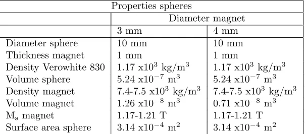
The structured particles are the part of the system which form the actual structure. It is critical for successful self-assembly that the particles contain the right information to enable the formation of the intended structures. The shape of the particles is a controllable parameter to exclude unwanted energy minima. The particles we chose are spheres and tetrapods. Neodymium magnets were fitted inside the particles to provide an attractive force, see section 3.2. The process of 3D-printing enabled a clean and quick production of the particles. The particles were printed at the Control Engineering group at the University of Twente. The material used is Objet Verowhite 830. This is an opaque white plastic. The properties of the used spheres are shown in table 3.2.

Spherical particles were chosen because of their relatively simple structure, see figures 3.2 and 3.3. Mathijs Marsman already did a number of experiments with these spherical particles [Marsman 2012]. The particles enable us to verify the characteristics of the setup since there were revisions since the previous experiments were done. The spherical particles consist of 2 halves with a extruded cut for the fitting of the magnet. They are assembled by glueing them together.

Properties spheres

Diameter magnet

3 mm 4 mm

Diameter sphere 10 mm 10 mm Thickness magnet 1 mm 1 mm

Density Verowhite 830 1.17 x103 _kg/m3 _{1.17 x10}3 _kg/m3

Volume sphere 5.24 x10−7 _m3 _{5.24 x10}−7 _m3

Density magnet 7.4-7.5 x103_kg/m3 _{7.4-7.5 x10}3_kg/m3

Volume magnet 1.26 x10−8 _m3 _{0.71 x10}−8 _m3

Ms magnet 1.17-1.21 T 1.17-1.21 T

Surface area sphere 3.14 x10−4 _m2 _{3.14 x10}−4 _m2

Table 3.2: Properties of the used spheres.

Tetrapods were chosen because of their potential to form a diamond like structure. Figures 3.4 and 3.5 show the structure of the tetrapods used in the experiments. A tetrapod has 4 pods fitted with neodymium magnets. Two pods have a magnet with its northpole facing outward and two pods are fitted with their northpole facing inward. The tetrapods are build from a centerpiece, four magnets and four caps encapsu-lating the magnets in the tetrapod. The magnetic binding strength of the tetrapods is determined by the strength of its magnets and the length of the caps. If the length of the caps increase, the magnetic energy decreases inversely with roughly 1/z3_{withzthe distance between magnets. The properties of the tetrapods}

Properties tetrapods

4/5 mm 5/5.5 mm Diameter pod 10 mm 10 mm Height tetrapod 19 mm 19 mm Diameter magnet 4 mm 5 mm Thickness magnet 1 mm 1 mm

Density Verowhite 830 1.17 x103 kg/m3 1.17 x103 kg/m3 Volume tetrapod 2.53 x10−6 m3 2.68 x10−6 m3 Density magnet 7.4-7.5 x103_kg/m3 _{7.4-7.5 x10}3_kg/m3

Volume magnet 1.26 x10−8 _m3 _{1.96 x10}−8 _m3

Ms magnet 1.17-1.21 T 1.17-1.21 T

Thickness cap 5 mm 5.5 mm Surface Area 2.42 x10−3 _m2 _{2.56 x10}−3 _m2

Table 3.3: Properties of the used tetrapods.

The particles used are submersed in water and they are not in a steady state, since water and air bubbles are flowing around them and throwing them around. It is useful to determine the Reynolds number. The Reynolds number describes the ratio between viscous and inertial forces in fluidic systems and gives a measure in the laminarity or turbulence of a system [Purcell 1977]. The Reynolds number is a dimensionless number. It is possible to determine this ratio for a sphere in a fluid. The Reynolds number is described by equation 3.1.

Re ≡

Finertial

Fviscous

∼d vρ

η (3.1)

Wheredis a characteristic distance. In the case of a sphere in a fluid,dis the spheres diameter. Parameter

v is the characteristic speed of the particle, η is the dynamic viscosity of the fluid,ρ is the density of the fluid.

Figure 3.3: Photograph of the spheres with a diameter of 10 mm and a magnet of 4 mm diameter and 1 mm thickness.

Figure 3.4: Illustrations of a tetrapod with 5 mm diameter magnets and 5.5 mm caps. The top face of the magnet is 5 mm apart from the top face of the cap. Left is assembled and right is in exploded view.

Figure 3.5: Photograph of tetrapods as used in this thesis. The tetrapods shown are fitted with 5 mm diameter neodymium disk shaped magnets and 5.5 mm caps.

3.2

Binding force

in the environment. At the microscale there can be thousands or even more. At the macro scale this is not practical because of the size of setup you would need to inhibit thousands of particles at a cm scale. A long range attractive force and accurate bonding is preferable, therefore a magnetic force seems to be the right force to use in this situation as an attractive force.

The magnets that we use for the magnetic attraction are disk-shaped N35 quality neodymium magnets with diameters of 4 and 5 mm and a thickness of 1 mm. Characteristic properties of these magnets are shown in table 3.4.

Br(T) Hc(kA/m) Max Min Max Min 1.21 1.17 899 876

Table 3.4: Magnetic properties of neodymium magnets of quality N35. Br is the residual flux density or remanent magnetic field. Hcis the coercive force.

To get a picture of the strength of the magnetic bonds and their energy is it useful to consider the magnetic theory describing these strengths and energies. Modelling the fields of disk-shaped magnets however is not straightforward. The easiest way to calculate the energy of the magnetic field would be to assume the magnets as magnetic spheres that behave like dipoles.

For a single magnetic sphere of radius a with a constant, spatially homogeneous magnetization, M, a magnetic field is generated identical to that of a point dipole with a magnetic moment given bym=µ0VM

withV = 4 3πa

3_.

H=3(m·ˆr)ˆr−m 4πµ0r3

(3.2)

In this equationˆr=_rrdenotes the unit vector parallel tor. The magnetic energy is given byUm=−m·H

where H is the external field caused by a neighboring dipole. The dipole experiences a force which equals

F=∇(m·H). Now the dipole-dipole energyUdd is equal to the work needed to bring the two dipoles with

moments,m1 andm2, from infinity to separation,r[Bishop 2009].

Udd=

m1·m2−3(m1·ˆr)(m2·ˆr)

4πµ0r3

(3.3)

The assumption to describe the magnetic field of a disk-shaped magnet is correct if the distance between two disk-shaped magnets is far enough. The exact solution for close separation however is different from the approximation of a dipole-dipole interaction as shown in figure 3.6. The magnetostatic force acting on a dipole is obtained byF =−∇Um. To get a more accurate simulation the exact fields have to be taken

into account. Equation 3.4 is used to minimize the magnetostatic energy with H = B/µ0. The dipole

moments are allowed to rotate in the direction of the net field and the resultant fields are calculated at each iteration step ∆t. αis a damping factor which is manually adjusted to optimize simulations speed but still maintaining convergence [Alink 2011].1

∆m

∆t =−αm×(m×H) (3.4)

Figure 3.7 shows another approach. The dipole - dipole approximation is shown and also the surface charge integration approach which is much more accurate. The dipole - dipole approach can be used from a distance of about 40 mm. At a distance of 40 mm the difference between the exact and the dipole approximation is 7%. This means we have to use the exact fields of disk-shaped magnets if the distance of separation is any closer.

Figure 3.6: Simulations of the force between two cylindrical magnets as a function of center to center separation. Solid line is the exact solution, dashed line is the dipole approximation. Taken from [Alink 2011].

3.3

Environment

The environment used for the self-assembly of the tetrapods and spheres consists of a confined container which provides a physical boundary condition. Another important part of the environment is the medium in which the particles move. Water was chosen as the environment for the particles because of the small relative difference in density, the availability of it and the ease of working. Gravity is another part of the environment, it is responsible for pulling the particles down to the bottom of the setup. The difference in density between the particles and the water is too large to let the particles float on their own. At the bottom of the setup there is a two dimensional situation but we want three dimensional self-assembly. To get the particles moving and hovering an upward flow of water is provided to counteract the gravity.

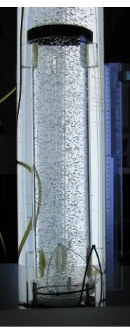
The setup used for the experiments is shown in figures 3.8 and 3.9. The setup consists of a perspex tube with a diameter of 20 cm filled with water. Inside this tube there is a smaller tube submersed with a diameter of 10 cm and a length of 58.5 cm. The distorting energy or air bubbles are provided through a porous stone, often seen in aquaria, which acts as a diffuser. The amount of air provided to the system is controlled by a flowcontroller by Bronkhorst High-Tech of the type E-5752-AAA and a mass/flow sensor by Bronkhorst High-Tech of type EL-Flow F-201C-FA-22-V. The flow of air also controls the flow of water needed to let the particles hover. In order to have some control over the flow of water a setup was made to control the distanceabetween the diffuser and the innertube, see figure 3.10. The height of the diffuser can be adjusted by adjusting the nuts on the three threads. The flow of water is presumably caused by the difference in density between the water outside the innertube and the solution of water and air inside the innertube or by a Venturi like effect. Some thoughts on the Venturi effect in this setup and an analysis by Mathijs Marsman on the density of the mixture of water and air may be found in appendix D.

The particles are kept inside the innertube through the use of filters at the bottom and top of the innertube. The setup was lighted by 2 high frequency light sources to enable flicker free imaging. The characteristics of the setup used are shown in table 3.5.

Properties setup

Temperature 294 K Density water at 294 K 998 kg/m3

Dynamic viscosity water at 294 K 1.002 x10−3 _{Pa s}

Height innertube 0.585 m Volume innertube 3.66 x10−3 _m3

vth 0.23 m/s

Gravitational constant 9.81 m/s2

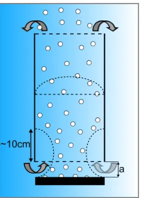
Figure 3.8: A schematic view of the setup used to perform self-assembly. Airbubbles (white circles) are pumped through the diffuser placed under the innertube and agitate the particles (red circles). The particles are in the cm scale. The flow of water (the grey arrows) needed to let the particles hover is generated by the upward flow of airbubbles. We have proven that the distanceabetween the diffuser and the innertube controls the flow of water into the innertube. The optimal value for our experiments wasa= 1.5 cm.

3.4

Driving force

Driving forces are the engine behind self-assembly. These forces are preferably random in order to move the particles around and let them collide. The driving forces are there to provide the mobility needed for successful self-assembly.

Brownian movement is the random movement caused by thermal noise at the micro scale. Brownian movement or random walk is shown in equation 3.5.

< R2>= 6kT

µ t (3.5)

< R2>Is the square distance of the movement which is proportional to the timetelapsed. 6kT Is the energy provided by the thermal bath or noise. µIs the mobility of the particles [Feynman 1970]. To enable a stochastic driving force at the macro scale we use air bubbles driven through the setup. The air bubbles collide with the particles in the system and cause them to move randomly. This is somewhat analogue to Brownian motion. On a microscopic scale, the average kinetic energy in a thermodynamic system is fixed at

1

2kT[Elwenspoek 2010]. At a macroscopic scale energy is continuously dissipated towards the thermal energy

of the system and distributed over all macroscopic degrees of freedom. The agitation at macroscopic scale is in contrast to thermal noise at the microscopic level in a particular frequency band and will have a certain general orientation and amplitude. This is also the case in the experiments conducted for this thesis. The distorting energy put into the system will have a non random component in the upward direction because the air bubbles travel mainly upward. This is due to their buoyancy. The distorting energy provided is assumed to be linear with the flow of air through the system, see equation 3.6 [Marsman 2012].

ED=aQair (3.6)

The distorting energy is denoted byEd. Parameterais a proportionality factor andQair is the airflow.

3.5

Boltzmann distribution

The driving forces in self-assembly are preferably stochastic. The random nature of these forces makes it difficult, if not impossible, to predict how and if the system will self-assemble and to what degree. However if it is possible to statistically describe a system with a Boltzmann distribution, we can calculate the probability to find the system in a certain state. The Boltzmann distribution in its general form looks like 3.7 withZ(T) the partition function. The Boltzmann distribution essentially describes the probability to find a fraction of particles in a system occupying a certain state with energyEi. The degeneracy of energy stateEi is shown

bygi. The Boltzmann constant iskandT is temperature of the system. EssentiallykT is the thermal bath,

the provider of distorting energy, of the system.

Ni

N =

gie−Ei/(kT)

Z(T) (3.7)

Z(T) =X

i

gie−Ei/(kT) (3.8)

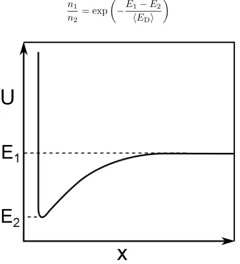
Figure 3.11 shows the potential energy (U) landscape of for example two magnets separated a distancex

from each other. There are two stable situations. When the two magnets are far apart, distancexis large, the mutual attraction of the magnets is too small to bring them together. The energy of this state converges to a value which we call E1. The number of particles in the state with this energy is n1. Particles in this

physical barrier formed by the plastic cover in which the magnets are fitted. For the spherical particles this is the half of a sphere. For the tetrapods this ideally is the cap which is placed on the centerpiece. This potential energy minimum is the other stable state of the system with two particles. We call this state the state with energyE2. The number of particles in this state is n2. The only way to get the particles from

the assembled state to the disassembled state is to provide kinetic energy to the system. This kinetic energy is the distorting energyED. At the micro scale this is thermal noise, at the macro scale in this thesis it is

provided through the air bubbles agitating the system. The energy needed to disassemble the two particles is ∆E =E1−E2. We are able to setup a Boltzmann distribution. The ratio of n1 and n2 is determined

by the exponential of the ratio of ∆E and the distorting energy ED. Equation 3.9 shows the Boltzmann

distribution of the system with two magnetic particles. Things get more complicated when there are more potential energy minima in the system. This may be due to more particles in the system or more magnets per particle like in tetrapods. Also the shape of the particles come into play enabling or prohibiting unwanted potential energy minima.

One of the goals of this thesis is to find out whether this simple Boltzmann distribution is valid for our system.

n1

n2

= exp

−E1−E2 hEDi

(3.9)

Figure 3.11: Schematic representation of the potential energy landscape which most likely is encountered in magnetic self-assembly with two magnets. At the vertical axis the potential energy is shown. At the horizontal axis a distance is shown. At energy state E1 the magnets are far apart and do not attract each

other. At energyE2 the magnets have attracted each other and run into an energy barrier formed by the

coating of the magnets or in our case the plastic material of the particles. There are two distinct states of energy. This enables us to use a Boltzmann distribution.

3.6

Self-assembly kinetics

There are three different reaction steps which occur in the process of self-assembly. First there is a forward reaction in which the attractive forces are larger than the repulsive forces. This leads to combining of two or more particles into another energy state. Second there are state changes. State changes are conformational or internal changes in the already assembled body. For example in the case of a tetrapod dimer: the concentric rotation of one tetrapod with respect to another attached tetrapod is an internal change. The state of energy of the configuration changes but the centers of mass remains intact. Last there is a backward reaction in which the cluster dis-assembles, because repulsive forces are dominating over the attractive forces. The balance of forces determines whether a structure remains assembled.

If there are two particles fitted with magnets inside a system it is possible to describe the combination and separation rate and their ratio K. We assume there are two states possible in the system with two particles, connected or disconnected. We do not take into account internal state changes because they do not change the structure of the particles. The ratio between the two states are determined by the rate of separation, kseparation, and the rate at which the particles meet each other, the rate of combination,

kcombination[Marsman 2012].

K=N◦↔◦

N◦◦

= kseparation

kcombination

(3.10)

The rate of separation depends on the ratio between the magnetic energy of the two magnets together

EMand the energy of the collisionEcollision of an air bubble with either one of the particle. ConstantAis a

scaling factor and corrects for matters like drag and density [Marsman 2012].

kseparation=Aexp

− EM

Ecollision

(3.11)

The energy of a collision between a particle and a bubble of air is shown by equation 3.12. We assume the energyEcollision to be linear to the flow of airQair provided in the system. Wherecis a proportionality

factor [Marsman 2012].

Ecollision=c Qair (3.12)

The combination rate of particles in a system depends on the diffusion of the particles. It describes the chance particles meet. The distorting energy ED is provided through the air bubbles. The diffusion

coefficient is denoted by D. The effective radius of the particle is rparticle. The dynamic viscosity of the

liquid isη. The mean free pathl is a ratio of the volume of the pipe in the setup and the range in which the 2 particles magnetically interact, see equation 3.14 [Feynman 1970], [Marsman 2012].

kcombination=

D l2 =

ED

6πηrparticlel2

(3.13)

l= Vpipe

πr2 attraction

(3.14)

Now it is possible to compare pairs of particles with two different magnetic energies and find out whether the model proposed by Mathijs Marsman is correct. For two pairs of particles with different magnetic energies we are able to supply the same distorting energy ED and thus we are able to compare the two situations.

To do this we rewrite the equations stated above. First we fill out equation 3.10 as shown in equation 3.15 and rewrite it into equation 3.16.

K=Aπηrparticlel

2

ED

exp

− EM

Ecollision

(3.15)

ED=

Aπηrparticlel2

K exp

− EM

Ecollision

There are two different particles, we assume the characteristic radius for both particles to be almost the same, they are both in the cm scale. We assume scaling factorA to be constant for both particles. There will be small differences in geometry and thus drag forces for both particles. We assume the difference to be small. There will be a difference in the ratioK. We useK1 andK2 to denote the different ratios for the

different particles. The same goes for the magnetic energiesEM1 andEM2. We assume the collision energy

Ecollisionto be the same for both particles. The dynamic viscosity does not change, the environment remains

the same. There will be a difference in the range in which a pair of particles attract each other because of the difference in diameter of disk-shaped magnets. Therefore we will usera1 andra2to denote the different

attraction lengths for the different particles. Now we are able to put up the equations for the two different pairs of particles and equal them to each other, see equation 3.17.

Aπηrparticle _V pipe πr2 a1 2 K1 exp

− EM1

Ecollision = Aπηrparticle _V pipe πr2 a2 2 K2 exp

− EM2

Ecollision

(3.17)

Which rewrites into equation 3.18.

1

K1r4a1

exp

− EM1

Ecollision

= 1

K2r4a2

exp

− EM2

Ecollision

(3.18)

We rewrite equation 3.18 into equation 3.19. The model by Mathijs assumes Ecollision to be linear with

the airflowQair. We rewrite equation 3.19 into equation 3.20 and then to the final equation 3.21. Now it is

possible to see if the assumption of linearity inEcollisionwith the airflow Qairis correct, see section 4.4.

exp

_E

M1−EM2

Ecollision

= K1

K2

r_a14 r4

a2

(3.19)

EM1−EM2

Ecollision

= ln

_K1

K2

+ 4 ln

_r

a1

ra2

(3.20)

Ecollision(Qair) = (EM1−EM2)

ln

_{K1 (Q}

air)

K2 (Qair)

+ 4 ln

_r

a1

ra2

−1

4

Results and Discussion

In this chapter the results of the various experiments are iterated and conclusions are taken. The density of the particles used in the experiments was measured, the results can be found in appendix A. The magnetic field of the neodymium magnets used in the particles was measured and their saturation magnetization was calculated, the results of these measurements and calculations can be found in appendix B .

4.1

Reynolds number of tetrapod

Figure 4.1: The figure shows the calculated range of the Reynolds number of a tetrapod. A tetrapod is assumed to behave like a sphere in a fluid. The minimum diameter is that of a spherical particle with a diameter of 10 mm. The maximum diameter is that of the envelope sphere of a tetrapod with 5.5 mm caps which is around 20 mm.

Figure 4.2: Schematic view of a tetrapod with two radii denoting the centerR1 and the envelopeR2 of the

tetrapod. The characteristic length of a tetrapod is expected to lie betweenR1 andR2.

4.2

Interaction of 2 magnetic spheres

Because of the adjustments made to the setup it is necessary to perform some verification with previous work done by Mathijs Marsman [Marsman 2012] to see whether the setup still has the same characteristics. To this end two spherical particles with a diameter of 10 mm and fitted with neodymium magnets of 3 mm diameter and 1 mm thickness are placed inside the setup and the number of connected pairs was counted out of a 100 photographs at several airflows. The distanceafrom the innertube to the diffuser providing the airflow was 1.5 cm. The results of dimer versus airflow are shown in figure 4.3.

the distorting energy and the system can be described by a Boltzmann distribution. The distorting energy will become larger than the potential energy barrier and causes the pair of particles to disassemble. We see from the results that our expectation is met. A higher airflow leads to less dimers and so we may conclude the distorting energy increases with increasing airflows. The results show a trend similar to the results obtained by Marsman [Marsman 2012].

Figure 4.3: Plot of the measurements of the interaction of 2 spheres with a diameter of 10 mm fitted with disk-shaped magnets of 3 mm diameter and 1 mm thickness at different airflows. The distanceafrom the innertube to the diffuser is 1.5 cm. The line is a guide to the eye.

4.3

Average height of particles

Distanceais the distance between the innertube and the diffuser. There is a dependence of distanceaon the upward flow of water caused by the upward flow of air inside the tube. It is possible to influence the average height of a particle in the system by changing the distanceawhile maintaining the range of distorting energy provided through the airflow.

One sphere with a diameter of 10 mm and fitted with a neodymium magnet of 4 mm diameter and 1 mm thickness was placed inside the innertube. A range of airflows was applied. At each airflow 50 pictures were taken with a ruler next to the setup. Afterwards the pictures were analysed to determine the height of the particle statistically. The procedure was repeated for three different distancesa.

Figure 4.4: Schematically shown is the development of the flow profile inside the innertube. Above approxi-mately 10 cm the mixture of air and water is ’homogeneous’. Below 10 cm the air bubbles are concentrated in the middle of the innertube by the inflow of water from the side. The velocity profile of the waterflow is inhomogeneous along a cross section of the tube.

The results of the average height measurements are shown in figure 4.5 and 4.6. The number of measure-ments per airflow per distanceawas statistically indeterminate. Therefore the average height of the particle was binned. The tube was divided in two bins. The lower bin ranged from 0 to 29.25 cm and the upper bin ranged from 29.26 to 58.50 cm. The number of times the particle was found in the lower bin at different airflows for different distancesais shown in figure 4.5. For all distancesathe number of particles in the lower bin decreases as the airflow increases. This happens around an airflow of 43.6 x10−6_m3_{/s and for increasing}

airflows. Below this value there seems to be not enough upward flow to lift the particles into the upper half of the tube. For larger distances ofathe number of particles in the lower half of the system decreases more rapidly at increasing air flows. This indicates an increase in the upward flow of water for increased distances of a. There should be a decrease in upward flow with increasingaif the upward water flow were to be dependant on the Venturi effect. Consequently, the upward water flow is not a result of a Venturi like effect, which we originally suspected. The number of particles in the lower half of the setup for differenta

are shown in figure 4.6 for an airflow of 61.1 10−6_m3_{/s. The upward waterflow increases with increasinga.}

The upward flow of water is most probably caused by the difference in density between the water outside the innertube and the mixture of water and air inside the tube. The distanceamay be limiting the amount of water able to flow into the innertube. The distanceato be chosen depends on the density of the particles used and the range of distorting energy needed. In the remainder of this thesis a distance aof 1.5 cm was chosen as it enabled a range of distorting energies without lifting the particles into the upper filter of the setup.

Figure 4.5: Measured result of the number of spheres in the bottom half of the innertube (0 - 29.25 cm) at different airflows and different distancesa are shown. Measured out of 50 photographs. The black squares indicate a distance a of 1.5 cm, the red circles indicate a distance a of 2.5 cm, the blue triangles were measured at a distanceaof 4 cm. Up to an airflow of 43.6 10−6_m3_{/s there seems to be insufficient upward}

water flow to hover the sphere into the upper half of the innertube (29.25 - 58.5 cm). Higher airflows do provide enough upward water flow to get the sphere to hover in the upper half of the innertube. If distance

aincreases, the upward water flow increases.

Figure 4.6: This figure shows the number of times measured out of 50 photographs at which a sphere of 10 mm diameter fitted with a 4 mm diameter magnet was found in the bottom half part of the setup. The bottom half of the setup is between 0 and 29.25 cm. For different distancesabetween the innertube and the diffuser. The airflow is at 61.09 x10−6_m3_{/s. The number of spheres in the bottom half decreases as distance}

aincreases. This means the upward flow inside the innertube increases when distanceaincreases.

Figure 4.7: Average heights measured for a sphere and a tetrapod compared. The experiment is done by putting one particle in the system at different airflows and than measuring the height at set intervals of 5 seconds. Sphere diameter is 10 mm with 4 mm diameter magnet (Red squares), density is 1.34 ±0.17 x103_kg/m3_{. Tetrapod with 5 mm diameter magnets and 5.5 mm caps (Blue circles), density is 1.29±0.08}

x103_kg/m3_{. The errorbar is from the standard deviation although there is no normal distribution.}

4.4

Interaction of two tetrapods

Two different pairs of tetrapods were used. One pair was fitted with 5 mm diameter neodymium magnets and 5.5 mm caps. The other pair was fitted with 4 mm diameter neodymium magnets and 5 mm caps. The goal of this experiment is to find out whether the collision energyEcollision as mentioned in section 3.6 is linear

with the airflow. We use two pairs because we are then able to calculate this without using the distorting energy ED as it is currently unknown. The distance a was 1.5 cm. The pairs were put into the system

separately. At several airflows 100 pictures were taken with steady intervals of 5 seconds. Afterwards the pictures were analysed and the number of dimers counted. Figure 4.8 shows the results of this experiment. The number of tetrapods in the assembled state decreases when the distorting energy increases. This is expected, because as the distorting energy increases there is more energy available to drive the particles over the potential energy barrier of the bond between the tetrapods. Even though the caps on the 4 mm tetrapods are shorter, the pair of tetrapods fitted with the 5 mm diameter magnet shows a stronger binding strength over the whole range of airflows. The number of dimers fitted with 5 mm diameter magnets is larger than the pair of tetrapods fitted with the 4 mm diameter magnets. It should be noted that the measurements of the tetrapods with the 5 mm magnets in figure 4.8 are averaged over three measurements. The measurement of the tetrapod pair with 4 mm magnets is a singular measurement. This was due a lack of time.

We are able to check whether equation 3.21 is valid for our system. We expect a linear plot of the collision energy versus the airflow. There is an overlap in distorting energy for both pairs of tetrapods. The magnetic energy of the assembled state can be calculated. The magnetic energy EM1 of two tetrapods fitted with

disk-shaped magnets with a diameter of 5 mm and a thickness of 1 mm spaced 10 mm apart is calculated by Laurens Alink to be -5.65 x10−5 _{J. The six outer magnets are assumed to behave like dipoles. This}

assumption is accurate, see figure 4.10. The position of the outer magnets relative to each other is taken to be the position of energy minimum. Observations show this is a good approximation, also see figure 4.12. The magnetic energy EM2 of the same configuration but with 4 mm disk-shaped magnets spaced 9 mm

apart is calculated to be -3.04 x10−5 J. The values ofrattraction for both pairs of tetrapods and the value

at which the particles do not ’feel’ each other, is when the magnetic energy of the 2 disk-shaped magnets goes above -1 x10−6 J. For the 5 mm magnet ra1 = 0.038m. For the 4 mm magnet ra2 = 0.028m. The

ratioK is calculated from the number of dimers measured at the different airflows. The result is shown in figure 4.11. We expected a linear relation between the collision energy and the airflow. This linear relation is not apparent. Possible explanations for this non-linearity are. There may be a deviation from the actual magnetic energies of the dimers and the calculated values. We assumed parameter A from equation 3.17 to be equal for both tetrapods. The deviation inA will be small as drag and density are not significantly different between particles, also see A.1. The range of attraction of the particles may be wrongfully chosen, but the linearity ofEcollision should not change. Although observations have showed that the orientation of

the tetrapods relative to each other is often near the position of the energy minimum as shown in figure 4.10, measurements on the orientation of the tetrapods have to be done. This is, because the orientation of the pods on the outside of the structure relative to each other has an influence on the magnetic energy of the structure. Another possibility is the inability to describe the system with reaction kinetics as proposed by Marsman, and described in section 3.6. More measurements have to be done to obtain statistically reliable results and to be able to obtain a more definitive conclusion.

Figure 4.9: Comparison of the calculated magnetic energy of two different pairs of magnets. 5 mm Diameter magnets are shown in red circles. 4 mm Diameter magnets are shown in black squares. The distance between two magnets iszs. There is a difference in the distance of attraction for the two different pairs of magnets.

Figure 4.11: The figure shows the measured values of Ecollision for several airflows. These are calculated

through equation 3.21. A linear relation betweenEcollision and the airflow was expected. The linear relation

was not observed, which is currently under investigation.

4.5

Self-assembly with 8 tetrapods

One of the goals of this research is to find out whether our process of self-assembly can be described by a Boltzmann distribution. The correct balance between driving and binding forces could enable the formation of diamond-like crystal structures. These results could be extrapolated to the micro scale, as Boltzmann distributions are independent of scale. 8 Tetrapods fitted with 5 mm diameter neodymium magnets and 5.5 mm caps were placed in the setup at several airflows to investigate the balance between driving and binding forces. The process of self-assembly was statistically researched. The self-assembly process was captured by video. These videos were then statistically analysed. The structures present in the system at constant intervals of time were noted. For each distorting energy 100 intervals were analysed. The distanceawas 1.5 cm. Figure 4.13 shows the result of this study. Only the configurations without defects, and therefore useful for the formation of crystal structures are shown. The configurations without defects are the structures in which the faces of the pods are properly aligned with respect to each other. For examples of pictures of configurations with and without defects, see appendix C. The occurence of hexamers, heptamers, and octamers without defects was statistically indeterminate and therefore not included in figure 4.13. More measurements have to be done to get statistically relevant results for hexamers, heptamers, and octamers. As the distorting energy increases the number of dimers without defects increase. This is in contrast with the results found for the experiment with two tetrapods. A possible explanation is that for the two tetrapod system, dimers only can be formed by 2 monomers while the pool of structures for the eight tetrapod system to form dimers with is significantly larger. For trimers, tetramers, and pentamers the increase of structures without defects is insignificant with increasing airflow.

Figure 4.13: The observed occurrence of configurations of 8 tetrapods fitted with 5 mm diameter magnets and 5.5 mm caps useful for the formation of crystal like structures at different airflows. These are the structures without defects. Black squares are at 34.9 cm3_{/s, red circles are at 43.6 cm}3_{/s, blue triangles are}

at 52.4 cm3_{/s. Distance innertube to diffuser a was at 1.5 cm. Occurence of hexa-,hepta- and octomeres}

were statistically indeterminate because of their low occurrence.

is no shift observed in the ratio. The observed configurations have to be simulated and their magnetic energy calculated to confirm this.

Figure 4.14: This figure shows the ratio between configurations of 8 tetrapods fitted with 5 mm diameter magnets and 5.5 mm caps useful for the formation of crystal structures and all configurations including those not useful to the formation of crystal structures. The ratio was calculated from measurements at several airflows. Black squares are at 34.9 cm3_{/s, red circles are at 43.6 cm}3_{/s, blue triangles are at 52.4 cm}3_/s.

Occurence of hexa-,hepta- and octomeres were statistically indeterminate because of their low occurrence. Distance innertube to diffuserawas at 1.5 cm. The yield decreases as the order of the configuration increases.

We have observed tetrapods successfully self-assembling into chains with lengths up to 8 tetrapods. The formation of crystal structures has not yet been observed. Observations show that tetrapods preferably form chains as useful configurations. Branching as shown in figure 4.15 is rare. The formation of chains seems to be energetically preferable for useful configurations. Simulation and computing of the magnetic energy may confirm the preferability of straight chains over branching. Observed is that the bonds between tetrapods are often broken by interparticle interaction, which is the collision between particles or collision with the boundary of the setup. There is a possibility the tetrapods used do not contain enough information to successfully self-assemble into a diamond like structure. Our experiments indicate that there may be too many energetic states favourable next to the ’ideal’ state which allows the formation of configurations useful for crystal structures. Modelling of the magnetic energy of the different configurations with and without defects may prove insight in the potential energy landscape of the different configurations and how to avoid these unwanted energy minima.

Observations show that most bonds are broken in the bottom quarter of the system. In the bottom quarter of the system the mixture of air and water is not fully homogeneous. The distorting energy seems to be unevenly distributed through the system.

Figure 4.15: Photograph of five tetrapods fitted with 5 mm magnets and 5.5 mm caps forming a pentamer at an airflow of 52.4 cm3_{/s. The picture shown is one of the few showing a branching of the tetrapods.}

Branching like this is critical to form crystal like structures. The lines drawn into the picture represent pods and the red dots the connecting faces.

Figure 4.16: Photograph of eight tetrapods fitted with 5 mm magnets and 5.5 mm caps forming an octomer at an airflow of 52.4 cm3_{/s. Several defects are shown. The diameter of the innertube only allows the chain}

like structure to curl around its curvature indicating that the system is too small.

4.6

Lifetime of configurations with 8 tetrapods

The lifetime of the configurations made by self-assembly with tetrapods was measured. Eight tetrapods fitted with 5 mm diameter neodymium magnets and 5.5 mm caps were placed in the setup. The airflow was set at 34.9 cm3_{/s. The process of self-assembly was captured on video. The distance a was 1.5 cm.}

Figure 4.17: Shown is a measurement of the average lifetime of configurations of 8 tetrapods fitted with 5 mm diameter magnets and 5.5 mm caps useful for the formation of crystal like structures. Airflow was at 34.9 cm3_{/s and distance innertube to diffuser was at 1.5 cm. Lifetime of hexa-,hepta- and octomeres were}

5

Conclusions and recommendations

5.1

Conclusions

Successful self-assembly of tetrapods into chains with a length of 2 to 8 particles has been observed. Branching was also observed. This is an encouraging result as it shows that self-assembly is possible in our system. The yield of configurations without defects decreases as length of the chains increase. There is no clear trend in the yield of configurations without defects with increasing distorting energy. There is no clear trend in the average lifetime with increasing chain length.

The water flow in the setup increases with an increasing distance between tube and diffuser. An increase in airflow leads to an increase in water flow, which limits the range of distorting energy experimentally available in this system.

The Reynolds number for the particles used lies between 2000 and 5000, which means the flow around the particles is in between laminar and turbulent. It will be difficult to determine the airflow component of the distorting energy if turbulence adds to distorting energy provided by the airflow.

The distorting energy is unevenly distributed in the system, which adds complexity to the system. Experiments with 2 particles show that an increase in airflow causes less dimer formation for spheres and tetrapods. Therefore we have confirmed that the distorting energy increases by increasing the airflow. Controlling the amount of distorting energy through the airflow is viable.

The number of tetrapod dimers increases with increasing interaction force.

In a system with 8 tetrapods the number of tetrapod dimers increases with increasing distorting energy.

5.2

Recommendations

There are several recommendations with respect to the setup in which the self-assembly occurred. Firstly a larger setup is needed to give the particles more space to self-assemble into larger structures. Secondly there should be separate control of water flow and airflow in order to have a better control over the distorting energy and the average height of the particles. Thirdly the velocity profile of the upward flow of water has to be stabilized to find out whether a normal distribution in height for the particles is possible. Stabilization of the velocity profile could be done by applying a filter of small tubes or straws. This filter may also enable a more homogeneous distribution of distorting energy. Fourthly a tracking system for three dimensions with two cameras would be useful as the time needed to gather statistics from video material and photographs is time-consuming.

Bibliography

[Abelmann 2009] Abelmann, L., Tas, N. R., Berenschot, J. W., and Elwenspoek, M. C. (2009). ”Self assem-bled three-dimensional nonvolatile memories”. Technical Report TR-CTIT-09-29, Centre for Telematics and Information Technology University of Twente, Enschede.

[Alink 2011] Alink, L., Marsman, G. H., Woldering, L. A., and Abelmann, L. (2011). ”Simulating three dimensional self-assembly of shape modified particles using magnetic dipolar forces”. pages 254–257, In Proceedings of the 22nd Micromechanics and Microsystems Technology Europe Workshop, Tonsberg, Norway, pages 254–257, Norway. Department of micro and nano systems technology, Vestfold University College.

[Bishop 2009] Bishop, K. J. M., Wilmer, C. E., Soh, S., and Grzybowski, B. A. (2009). ”Nanoscale forces and their uses in self-assembly”. Small,5(14):1600–1630.

[Elwenspoek 2010] Elwenspoek, M., Abelmann, L., Berenschot, E., Van Honschoten, J., Jansen, H., and Tas, N. (2010). ”Self-assembly of (sub-)micron particles into supermaterials”. Journal of Micromechanics and Microengineering,20(6).

[Feynman 1970] Feynman, R. P. (1970). The Feynman Lectures on Physics, volume 1. Addison Wesley Longman.

[Ilievski 2011] Ilievski, F., Mani, M., Whitesides, G. M., and Brenner, M. P. (2011). ”Self-assembly of magnetically interacting cubes by a turbulent fluid flow”. Physical Review E - Statistical, Nonlinear, and Soft Matter Physics,83(1).

[Marsman 2012] Marsman, M. (2012). ”Msc thesis”. in preparation.

[Munson et al. 2010] Munson, Young, Okiishi, and Heubsch (2010). Fundamentals of Fluid Mechanics. Wi-ley.

[Pelesko 2007] Pelesko, J. A. (2007). Self Assembly, The Science of Things That Put Themselves Together. Chapman & Hall/CRC.

[Penrose 1957] Penrose, L. S. and Penrose, R. (1957). ”A self-reproducing analogue [1]”. Nature,

179(4571):1183.

[Purcell 1977] Purcell, E. (1977). ”Life at low reynolds number”. American Journal of Physics,45:3–11. [Stambaugh 2003] Stambaugh, J., Lathrop, D. P., Ott, E., and Losert, W. (2003). ”Pattern formation in

a monolayer of magnetic spheres”. Physical Review E - Statistical, Nonlinear, and Soft Matter Physics,

68(2 2):026207/1–026207/5.

[Tomiyama 2002] Tomiyama, A., Celata, G., Hosokawa, S., and Yoshida, S. (2002). ”Terminal velocity of single bubbles in surface tension force dominant regime”. International Journal of Multiphase Flow,

28(9):1497 – 1519.

[Whitesides 2002] Whitesides, G. M. and Boncheva, M. (2002). ”Beyond molecules: Self-assembly of meso-scopic and macromeso-scopic components”. Proceedings of the National Academy of Sciences of the United States of America,99(8):4769–4774.

[Woldering 2011] Woldering, L. A., Abelmann, L., and Elwenspoek, M. C. (2011). ”Predicted photonic band gaps in diamond-lattice crystals built from silicon truncated tetrahedrons”. JOURNAL OF APPLIED PHYSICS, 110(4).

Acknowledgements

List of Symbols

< R2_{> Brownian movement} B Magnetic induction

η Dynamic viscosity

ˆr Unit vector

F Force vector

H Magnetic field

m Magnetic moment

r Separation vector

µ Mobility

µ0 Permeability of vacuum

ρ Density

a Radius sphere

Br Residual flux density

D Diffusion constant

d Characteristic distance Reynolds number

E1 Energy of state 1

E2 Energy of state 2

Ei Energy of theith state

Ecollision Collision energy

EM1 Magnetic energy for tetrapod pair 1

EM2 Magnetic energy for tetrapod pair 1

EM Magnetic energy

ED Distorting energy

Finertial Inertial force

gi Degeneracy of theith state

Hc Coercive force

k Boltzmann constant

K1 Ratio disassembled/assembled for tetrapod pair 1

K2 Ratio disassembled/assembled for tetrapod pair 2

kcombination Rate of combination

kseparation Rate of separation

l Mean free path

N Number of particles

n1 Number of particles in state 1

n2 Number of particles in state 2

Ni Number of particles in theith state

N◦↔◦ Number of particles disassembled

N◦◦ Number of particles assembled

Qair Airflow

r Size of vectorr

ra1 Radius of attraction of tetrapod pair 1

ra2 Radius of attraction of tetrapod pair 2

rattraction Distance of attraction

Re Reynolds number

rparticle Effective radius particle

T Temperature

t Time

Udd Dipole-dipole magnetic energy

Um Magnetic energy

V Volume of sphere

v Characteristic speed

Vpipe Volume of pipe

Ms Saturation magnetization

A

Characterization of particles

The average weight and volume of the used particles were determined to calculate the density. The used particles are spheres and tetrapods as described in section 3.1. The weight was measured by weighing 10 particles on a mg scale. The volume was determined by filling a cylindrical glass with a volume of water. The reference volume was noted and ten particles were added to the volume of water. Air trapped to the particles was shaken out and the difference in volume with the reference was calculated. With the volume and weight known the density could be calculated byρ=m/V. The results are shown in table A.1.

Particle Avg Weight (kg) x10−3 _{Avg Volume (m}3_{) x10}−6 _{Avg Density (kg/m}3_{) x10}3

Sphere 4mm 0.70±0.02 0.52±0.05 1.34±0.17 Tetrapod 5mm/5.5mm 3.68±0.03 2.85±0.15 1.29±0.08 Tetrapod 4mm/5mm 3.33±0.02 2.60±0.15 1.28±0.08

B

Magnetization measurements

The neodymium magnets used in the spheres and tetrapods were measured at 2 distances from the face of the magnet with a gaussmeter type Model 615 and a hall probe type HTB1-0608. The distance between the face of the magnet and the hall probe was around 1.5 and 2 cm. We assume the magnetic field to be homogeneous at this height. The two measurement heights give information about the assumption of homogeneity of the magnetic fields. An xy-scanning table was used to scan the magnetic field in a grid with measuring points separated at 2 by 2 mm, see figure B.1. The setup used is shown in figure B.2. The position of the magnet relative to the hall probe was set by using the micrometer screws. The measured result of one of the 5 mm diameter magnets is shown in table B.1. The results are corrected for noise magnetism. Three magnets of the diameter 5 mm, and two magnets with a diameter of 3 mm and 4 mm were measured. Laurens Alink made it possible to determine the central axis of the magnets by extrapolating the field strength and search for a maximum, see figure B.3. The field profiles of disk shaped magnets are well known. The resultant field profile was then compared to simulated results, see figures B.4 and B.5. The results are shown in table B. The measurements of the magnetic saturation are compliant with N35 quality standards of neodymium magnets.

Figure B.2: The xy-scanning table used to characterize the neodymium magnets. The scanning motion was done by hand. The position can be adjusted by turning the micrometer screws.

x/y(mm) 0 2 4 6 8 10 12 14 0 -1.9 -2.4 -2.8 -3.1 -3.2 -3 -2.7 -2.2 2 -2.6 -3.3 -3.9 -4.3 -4.4 -4.2 -3.7 -3 4 -3.3 -4.2 -5 -5.6 -5.7 -5.4 -4.7 -3.8 6 -3.8 -5 -6 -6.7 -6.9 -6.5 -5.7 -4.5 8 -4.2 -5.5 -6.6 -7.4 -7.7 -7.2 -6.3 -5 10 -4.3 -5.6 -6.8 -7.6 -7.8 -7.4 -6.4 -5.1 12 -4 -5.2 -6.3 -7 -7.2 -6.8 -5.9 -4.8 14 -3.5 -4.5 -5.4 -6 -6.2 -5.9 -5.1 -4.2

Table B.1: Magnetization measurements on a neodymium magnet of quality N35 with a diameter of 5 mm and a thickness of 1 mm. The height of measurement was 15.7 mm±0.1 mm. The error of the Hall probe and gaussmeter is±0.05 Gauss. The values are corrected for a measurement with no magnet.

Figure B.4: The field profile of the same 5 mm neodymium disk shaped magnet as above measured at a height of 15.75 mm. The red crosses are the measured values. The blue line is the simulated field profile and the black plus is the analytic solution to the field profile. The saturation magnetization is at 876 kA/m.

D=5mm D=4mm D=3mm Ms (kA/m) Ms (kA/m) Ms (kA/m)

876 822 737

858 823 764

816 879 702

815 864 620

933 874

C

Tetrapod structures

Self-assembly of tetrapods into structures was observed. This appendix shows some of the configurations observed during the work of this thesis.

Figure C.1: Two tetrapods fitted with 5 mm magnets and 5.5 mm caps forming a dimer at an airflow of 52.4

cm3_/s.

Figure C.3: Three tetrapods fitted with 5 mm magnets and 5.5 mm caps forming a trimer at an airflow of 52.4cm3/s. The structure shown is a chain and is useful for the formation of crystal structures as there are no defects in the configuration.

Figure C.4: Three tetrapods fitted with 5 mm magnets and 5.5 mm caps forming a structure with defects. At an airflow of 52.4cm3/s.

Figure C.5: Three tetrapods forming a trimer with a ring like structure at an airflow of 52.4cm3_{/s. This is}